Building Energy Codes: A Case Study in Regulation and Cost-Benefit Analysis

Including energy codes in building codes is a policy option for reducing energy consumption that has received increased attention since the 1970s, driven by concerns about energy security and climate change. How much have such building energy codes helped reduce energy consumption, and are they wise policies from the standpoint of society broadly conceived? This chapter introduces the major questions in the area of energy efficiency regulations in the residential sector, and then illustrates an economic technique known as cost-benefit analysis (CBA) by examining a recently published economic analysis of Florida’s energy codes.¹Grant D. Jacobsen and Matthew J. Kotchen, “Are Building Codes Effective at Saving Energy? Evidence from Residential Billing Data in Florida,” Review of Economics and Statistics 95, no. 1 (March 2013): 34–49.

My intention in presenting the case study from Florida is to illustrate the main steps in CBA, which is widely used throughout regulatory analysis. This chapter thus can be used by students, teachers, policy analysts, and others who wish to know more about how CBA could be applied to any of the regulations discussed in this volume. The practice of CBA integrates skills from across the theoretical and empirical subfields of economics, and consequently the study of CBA presents an excellent opportunity for meaningful student research projects. In the conclusion, I provide guidance that should be useful to students and professionals beginning an original CBA, and to teachers who are guiding students in this exercise.

Economists generally agree that CBA is an essential tool for selecting efficient regulations. CBA is often a part of regulatory impact analysis. It has been required for major regulations at the federal level for decades, and—at the subnational level—more and more states and cities have started to apply CBA to their public decision-making processes. For example, CBA is used at the California Department of Transportation to allocate funds among competing roadway improvement proposals.²Matthew J. Holian and Ralph McLaughlin, “Benefit-Cost Analysis for Transportation Planning and Public Policy: Towards Multimodal Demand Modeling” (MTI Report 12-42, Mineta Transportation Institute, San Jose, CA, August 2016).

Building energy codes are a specific example of a more general category of public policies: technical and performance standards. Similar types of regulations exist for automobiles, appliances, buildings, construction equipment, and a host of other energy-consuming products. For example, the Corporate Average Fuel Economy (CAFE) program requires automobile manufacturers to achieve specified levels of fuel efficiency, as measured by miles per gallon.

Though performance standards like the CAFE standards are intended to be fuel-saving policies, they can have unintended consequences. As cars use less gasoline per mile, the effective price of driving falls and people drive more—this is the so-called rebound effect.³Kenneth Gillingham, “Rebound Effects,” in The New Palgrave Dictionary of Economics, edited by Palgrave Macmillan (London: Palgrave Macmillan, 2014). https://doi.org/10.1057/978-1-349-95121-5_2875-1. The increased driving causes congestion, pollution, and traffic accidents, which were not goals of the energy efficiency policy. It is even conceivable that more fuel-efficient vehicles could encourage suburban sprawl, as households find it easier to sustain car-based lifestyles.

Manufacturers of appliances from refrigerators to air conditioners have been required to meet increasingly tight standards since the 1970s. The average annual energy consumption of a refrigerator has fallen from 1,800 kilowatt hours in 1976 to 450 in 2001, a dramatic increase in efficiency.⁴Arthur H. Rosenfeld and Deborah Poskanzer, “A Graph Is Worth a Thousand Gigawatthours: How California Came to Lead the United States in Energy Efficiency (Innovations Case Narrative: The California Effect),” Innovations: Technology, Governance, Globalization 4, no. 4 (2009): 57–79. What is responsible for the rise in efficiency of cars and refrigerators? Regulation may have played a role, but—as Arthur Rosenfeld and Deborah Poskanzer note—“the other factor contributing to the sudden drop in refrigerator energy use in the mid-1970s was the advent of a new manufacturing technology, blown-in foam insulation.”⁵Rosenfeld and Poskanzer, “A Graph Is Worth a Thousand Gigawatthours,” 70. This example illustrates the empirical challenge of determining the independent impact of energy codes on energy demand by just examining trends in average fuel use. In the next section, I highlight two empirical techniques, randomized controlled experiments and multiple regression, that analysts can use to reach more accurate estimates of the causal effect of a policy on an outcome of interest.

State and local governments use energy codes to apply energy efficiency standards in the residential sector. We can distinguish between building codes in general and building energy codes in particular. Building codes cover many aspects of housing structures, including plumbing, accessibility, and safety. Energy codes are but one part of the overall set of regulations with which home builders have to comply.

California and Florida were among the first states to adopt building energy codes. Economists Kevin Novan, Aaron Smith, and Tianxia Zhou discuss how builders in California complied with the initial energy codes.⁶Kevin Novan, Aaron Smith, and Tianxia Zhou, “Residential Building Codes Do Save Energy: Evidence from Hourly Smart-Meter Data” (E2e Working Paper 031, E2e Project, June 2017). They calculate that building a 1,620-square-foot, fully compliant house in Sacramento would have cost $1,565 more than a noncompliant house (in 1980 dollars), owing to additional ceiling and wall insulation and to infiltration control (e.g., caulking and weather-stripping sources of air leakage). Its builders would have also been required to install a smaller air conditioner. Every few years, states with energy codes tend to strengthen them. Grant Jacobsen and Matthew Kotchen discuss how in Florida, a builder had multiple options for adjusting a home design feature to bring it into compliance when that state’s energy codes were strengthened in 2002.⁷Jacobsen and Kotchen, “Are Building Codes Effective at Saving Energy?” One option was installing low-emissivity windows, which would have increased costs of a standard Florida home by between $675 and $1,012.

The problem of asymmetric information, where a builder knows more about the home’s design than the home buyer or tenants do, provides a market failure rationale for building codes. It is not easy for a home buyer or renter to see how much insulation is behind the walls, for example, and so if buildings are less energy efficient than they would be in a world without these types of informational challenges, both building codes in general and energy codes in particular could be justified on efficiency grounds.

Another motivation for building codes is energy cost myopia, a form of behavioral bias. This refers to situations where home buyers do not account for the long-term energy costs when they buy a home—they consider only the up-front costs. These are situations where consumers are unable to rationally consider future costs. This chapter will introduce a concept called discounting, and we will see that energy cost myopia could be modeled as homeowners behaving as if they have an irrationally high discount rate. Of course, to the extent that discount rates reflect personal preferences, an analyst imposing the “correct” discount rate on a homeowner is an example of paternalism—and there is no consensus about what discount rate a homeowner “should” have. In chapter 13 of this volume, James Broughel discusses the topic of energy cost myopia in more detail.

While asymmetric information and energy cost myopia are two of the most prominent justifications for energy codes, there are also some ways codes could be counterproductive in terms of their intended purpose. The rebound effect, discussed above in the context of cars, also pertains to homes. If homes are more energy efficient, the occupants may use the air conditioner more than they otherwise would. They may decide to bake a cake on a hot day, whereas otherwise they would have postponed baking until the sun went down. It can be time consuming to open and close all the windows in a large home. If the home is energy efficient, a household may decide to just keep the windows closed and use the air conditioner all the time, whereas otherwise they would have opened and closed the windows on the basis of the outside air temperature.

Energy efficiency regulations could also be harmful if they lull voters into a sense of complacency regarding energy consumption. This is a political economy point, related to one made by economist Arik Levinson on a Freakonomics Radio podcast episode with Stephen Dubner.⁸Stephen J. Dubner, “How Efficient Is Energy Efficiency?,” February 5, 2015, in Freakonomics Radio, podcast, https://freakonomics.com/podcast/how-efficient-is-energy-efficiency-a-new-freakonomics-radio-podcast/. Voters seem unwilling to enact a carbon tax, perhaps because they assume the government is doing enough through energy efficiency regulations.

The subfield of economics known as public choice emphasizes the possibility of so-called regulatory capture. Perhaps the home builders that can most easily comply with energy codes (likely the larger builders with more ability to navigate regulations) lobby for making the codes stricter because they know this will make smaller builders less competitive. If the regulatory process is “captured” by private interests, this would obviously reduce the efficiency of the new construction segment of housing markets.

A final issue that has received increased attention recently is the issue of distributional effects. Are energy codes and CAFE standards more equitable than energy or carbon taxes? In the context of homes, economists Chris Bruegge, Tatyana Deryugina, and Erica Myers find that “building energy codes result in more undesirable distortions for lower-income households.”⁹Chris Bruegge, Tatyana Deryugina, and Erica Myers, “The Distributional Effects of Building Energy Codes,” Journal of the Association of Environmental and Resource Economists 6, no. S1 (2019): S95. In the context of automobiles, Lucas Davis and Christopher Knittel find that “fuel economy standards are more regressive than a gasoline tax with revenues returned lump sum.” They conclude that “it is difficult to argue for fuel economy standards on the basis of distributional concerns.”¹⁰Lucas W. Davis and Christopher R. Knittel, “Are Fuel Economy Standards Regressive?,” Journal of the Association of Environmental and Resource Economists 6, no. S1 (2019): S61.

A typical view among economists is that there are often ways of reducing energy consumption that are less costly than energy efficiency regulations. In the case of CAFE standards, most of the top economists would prefer a gasoline tax over fuel economy performance standards.¹¹Davis and Knittel, “Are Fuel Economy Standards Regressive?” Nobel laureate William Nordhaus writes about energy codes and related approaches that they “can supplement and buttress more comprehensive greenhouse-gas emissions limits or carbon taxes. However, they are inefficient because they require spending substantial sums for minimal impacts.”¹²William D. Nordhaus, The Climate Casino: Risk, Uncertainty, and Economics for a Warming World New Haven: Yale University Press, 2013), 261. There may be rationales for some energy codes, especially in a world where we do not have carbon taxes, but regulators should be sensitive to the costs energy codes impose on builders. The costs and benefits of energy codes are the topics of the next section.

Evaluating Building Energy Codes: A Case Study

This section describes a recent economic analysis of building energy codes in Florida, which was carried out by Grant Jacobsen and Matthew Kotchen.¹³Jacobsen and Kotchen, “Are Building Codes Effective at Saving Energy?” Jacobsen and Kotchen’s analysis (hereinafter referred to as the JK analysis) has a lot in common with cost-benefit analysis, one specific type of economic analysis. Other methods of economic analysis include economic impact analysis and fiscal impact analysis, which are often mistakenly described as CBA. One of the goals is to section is to describe what CBA is, so a reader will be able to recognize when an analysis that is described as a CBA is in fact something else.¹⁴The focus in CBA is on human welfare broadly conceived, while economic impact analysis and fiscal impact analysis are narrower and focus on specific impacts. For example, fiscal impact analysis may focus on the impact of some policy or program on the state government’s budget, while economic impact analysis may focus on the policy or program’s impact on GDP. CBA, on the other hand, recognizes that social welfare can go up even as state budgets and GDP go down. For an example of economic impact analysis, see Anoshua Chaudhuri and Susan G. Zieff, “Do Open Streets Initiatives Impact Local Businesses? The Case of Sunday Streets in San Francisco, California,” Journal of Transport Health 2, no. 4 (2015): 529–39. For an example of fiscal impact analysis, see Dennis P. Culhane, Stephen Metraux, and Trevor Hadley, “Public Service Reductions Associated with Placement of Homeless Persons with Severe Mental Illness in Supportive Housing,” Housing Policy Debate 13, no. 1 (2002): 107–63.

CBAs are typically carried out in one of two settings. First, government agencies may commission CBAs or carry them out themselves. These studies typically strive to be comprehensive and adhere closely to the principles of CBA, but the quality of government CBAs varies widely. Second, academic journals sometimes publish CBAs, and while these may be comprehensive, they are usually shorter than the government-sponsored analyses. One reason for this is that academic studies often focus on one specific aspect of the policy in question. For example, the focus of the JK study was empirically estimating the impact of policy on energy demand. Jacobsen and Kotchen carry out an economic analysis as a secondary part of their study—six paragraphs out of the 16-page article. The fact that the JK analysis has relatively few moving parts is a virtue for my purposes, because it makes it an ideal candidate for an introduction to CBA.

Most CBAs share a common set of general features. Leading textbook authors Anthony Boardman, David Greenberg, Aidan Vining, and David Weimer describe them in a widely cited list containing nine steps:¹⁵Quoted from Anthony E. Boardman et al., Cost-Benefit Analysis: Concepts and Practice (Cambridge: Cambridge University Press, 2017), 6.

1. “Specify the set of alternative projects.”
2. “Decide whose benefits and costs count (standing).”
3. “Catalogue the impacts and select measurement indicators.”
4. “Predict the impacts quantitatively over the life of the project.”
5. “Monetize (attach dollar values to) all impacts.”
6. “Discount benefits and costs to obtain present values.”
7. “Compute the net present value of each alternative.”
8. “Perform a sensitivity analysis.”
9. “Make a recommendation.”

This list, or minor variations on it, is widely used in the literature. For example, in the context of CBA of crime, the authors of one 2016 book describe an essentially identical list that has ten steps.¹⁶Matthew Manning et al., Economic Analysis and Efficiency in Policing, Criminal Justice and Crime Reduction: What Works? London: Palgrave Macmillan, 2016), 36. My own opinion is that steps 6 and 7 could be combined, making this a list of eight steps. I use this list to organize the discussion that follows.

Jacobsen and Kotchen examine a change to Florida’s energy codes. Florida initially adopted energy codes in 1978 and strengthened them in 2002. The details of Florida’s 2002 energy code change are complicated, but—as a simplification—JK frame the policy as requiring new homes to use more expensive windows with a low-emissivity (low-E) coating, which should in turn reduce electricity and natural gas demand. This requirement was expected to lower household energy bills.

In terms of CBA step 1, one set of alternatives facing policymakers in 2002 was to change the code (require low-E windows) or not to change it. This set has only two options, and Jacobsen and Kotchen do not discuss whether policymakers at the time considered stronger or weaker versions of the code or other completely different policy instruments to promote energy efficiency, such as taxes or cap and trade. If these alternatives were included in an analysis, the set of alternatives would be larger than two. Many government-sponsored CBAs specify multiple alternatives, while academic CBAs are often less comprehensive in terms of alternatives.

In CBA step 2, standing refers to whose preferences count. This is a deeply philosophical question, but it is usually decided in CBAs on the basis of practical considerations. For example, a CBA conducted by a government agency may count costs and benefits to US citizens only. However, some economists hold that all impacted parties should have standing.¹⁷Diana Fuguitt and Shanton J. Wilcox, Cost-Benefit Analysis for Public Sector Decision Makers (Westport, CT: Greenwood, 1999), 53. As we see next, the JK analysis incorporates negative externalities to third parties from the emissions produced by the burning of fossil fuels. Thus their implicit delineation of standing is a global one, although they do also consider a case where only the homeowner has standing, and a case that could be described as one where only citizens have standing.

CBA step 3 has to do with cataloging impacts. The JK analysis includes (1) the additional resources builders use in complying with the code, (2) the reduction in energy used by households, and (3) the reduction in negative externalities associated with producing the energy. Examples of these externalities include the suffering of third parties who breathe in sulfur dioxide produced during electricity generation and smaller catches for fishers because of ocean acidification caused by climate change. Other potential impacts that Jacobsen and Kotchen do not catalog include the impact of more or less comfortable indoor temperatures.¹⁸This impact was included in the analysis in Meredith Fowlie, Michael Greenstone, and Catherine Wolfram, “Do Energy Efficiency Investments Deliver? Evidence from the Weatherization Assistance Program,” Quarterly Journal of Economics 133, no. 3 (2018): 1597–644.

CBA step 4 has to do with predicting impacts. Empirical training in causal inference is critical to doing this step well. Correlation is not causation, and the researcher needs to determine what impact was actually caused by the policy. It is not enough to discover that energy use was lower in homes built after energy codes were strengthened, because it is possible that other things changed along with regulations. For example, if for some reason homes were smaller on average after the codes were strengthened, it might appear that the codes were responsible for an observed lower energy use, but in fact the reason was that the smaller homes required less energy to heat and cool.¹⁹For further discussion, see Matthew J. Holian, “The Impact of Building Energy Codes on Household Electricity Consumption,” Economics Letters 186, no. 108841 (January 2020): 1-4. In this piece I discuss the exact case mentioned here, where home size changes over time along with energy efficiency, and show how multiple regression techniques can be used to estimate causal effects in this setting.

One technique analysts use to estimate impacts is to get data and estimate impacts themselves. Another technique is to use “the literature.” By the literature, I mean all the studies that have been written on a particular topic. An analyst who searches these studies will find estimates of impacts that have been produced by others. Because impact estimation is such a crucial step in any CBA, I discuss methods for this step in more detail in the appendix.

Jacobsen and Kotchen used residential billing data to estimate a multiple regression model that found that the change in Florida’s energy code caused electricity consumption to fall by 48 kilowatt-hours (kWh) per month and natural gas consumption to fall by 1.5 therms. They then use the literature to find so-called plug-in values to estimate the size of reduced emissions. The four categories of emissions they include are carbon dioxide, sulfur dioxide, nitrous oxide, and particulates. Emissions factors are numbers drawn from the literature that are used to estimate the reduction in emissions from each energy source. For example, the JK analysis cites a study that found burning 1 therm of natural gas generates 0.006 tons of carbon dioxide. If households reduce natural gas use by 1.5 therms per month, carbon dioxide emissions will fall by 1.5 × 0.006, or 0.009 tons of carbon dioxide monthly.

CBA step 5 involves monetization—assigning a dollar amount to an impact to represent its social value. The stricter energy codes require builders to use low-E windows, and monetization involves valuing the additional resources that go into producing these windows. The JK analysis finds an estimate in the literature indicating the low-E windows are 10 percent more expensive than non-low-E windows, and calculates that the change to the code has added between $675 and $1,012 to overall construction costs for a standard home.

Note that the increase in construction costs might not exactly correspond to the social costs of the resources. For example, imagine that the window manufacturing company is a monopoly and there is only a trivial increase in its cost from producing the low-E windows. In that case the higher price paid by builders to the window manufacturer would be a transfer from the builder to the window manufacturer, not a social cost. Now, it is unlikely that the window producer is a monopoly, and the technique Jacobsen and Kotchen adopt for monetizing the impact seems very reasonable to me—but I construct this example to illustrate that there are cases where a researcher cannot just use market prices in the monetization step.

To monetize the energy use reduction impact, Jacobsen and Kotchen multiply the energy savings (48 kWh of electricity and 1.5 therms of natural gas per month) by the marginal price an average household pays (14.6 cents per kWh for electricity and $1.22 per therm for natural gas) to arrive at annual energy savings of $106.²⁰The details behind this calculation are 48 kWh × 12 months × 14.6 cents = $84 annual electricity cost savings. For natural gas, the calculation is 1.5 therms × 12 months × $1.22 = $21.96. Adding these together, $22 + $84 = $106, which is the value of the annual energy savings. As with the construction impact discussed in the preceding paragraph, this seems to be a reasonable way of monetizing the social value of the saved resources, but it may not be perfect. For example, if the energy price consumers pay incorporates government taxes, then the price consumers pay will overstate the social value of the resource savings, because part of the price is a transfer rather than a resource cost.²¹It is a subtle point, but the reason monetizing with market prices is appealing is because neoclassical perfect competition theory teaches us that price equals marginal cost. Perfect competition is a theoretical condition not always met in the real world, however, and there are times when the use of market prices is not appropriate. In these cases, analysts have to be creative in calculating a so-called shadow price, which is simply the true social value of an impact.

The third set of impacts that must be monetized are the four types of emissions. Carbon dioxide causes climate change and the other three are associated with public health problems. (Particulates—essentially soot—can cause asthma, for example.) Earlier I discussed how Jacobsen and Kotchen estimate that carbon dioxide emissions fall by 0.009 tons each month, or 0.108 tons annually, because of reductions in natural gas use. The social cost of carbon has been calculated by William Nordhaus as $31 per ton of carbon dioxide (in 2010 dollars);²²Nordhaus, William D. “Revisiting the Social Cost of Carbon,” Proceedings of the National Academy of Sciences of the United States of America 114, no. 7 (February 2017): 1518–23. thus one way of monetizing the reduction in natural gas use is by multiplying 0.108 by $31, yielding an annual climate change mitigation benefit of $3.35. Jacobsen and Kotchen do not report the marginal damage figures they used for carbon, but it is possible to calculate these values from the information they do present.²³Table 5 in Jacobsen and Kotchen, “Are Building Codes Effective at Saving Energy?” It turns out that they used a low estimate of $7.68 and high estimate of $93.70, in 2009 dollars; thus the $31 figure from Nordhaus lies on the lower end of the range they considered.²⁴Jacobsen and Kotchen’s table 5 indicated the low- and high-end figures for carbon dioxide reduction owing to a fall in natural gas use as $0.83 and $10.12, respectively. Thus the marginal damage figures are calculated as follows: $0.83 ÷ 0.108 = $7.68, and $10.12 ÷ 0.108 = $93.70. I have verified with the authors that these were the marginal damage figures they used, and I thank Matthew Kotchen for sharing his analysis file with me. Hence the high-end estimate of the social value of reduced carbon emissions from natural gas is 0.108 tons times $93.70, or $10.12 annually. The JK analysis applies different marginal damage estimates to each pollutant and each fuel source, and finds that all together, reductions in the four types of emissions, owing to a household’s lower electricity and natural gas demand, are valued at between $14.15 and $84.84 annually.

CBA steps 6 and 7 can be combined. Discounting refers to accounting for the fact that a dollar saved next year is not as valuable as a dollar saved now. Net present value (NPV) is the most widely used of several decision criteria in CBA. In fact, because the JK analysis was, strictly speaking, not a CBA, Jacobsen and Kotchen do not present NPV calculations. Instead they discuss three different types of payback periods. Besides NPV and the payback period, other decision criteria one sometimes encounters include the internal rate of return and the benefit-cost ratio. However, there are several advantages to NPV that make it the most widely used and accepted decision criterion.²⁵Fuguitt and Wilcox, Cost-Benefit Analysis. If NPV is positive, this indicates that the investment, policy, project, or program produces more benefits than costs over its lifetime.

Using all the numbers presented in the JK analysis and discussed up until now, it is possible to calculate the NPV of the change in Florida’s energy codes for a household in Gainesville: 

. 

We can write this another way by specifying a time horizon. Say t = 1 and T = 10. Then we can express NPV using the equation below, which is less compact but avoids the use of the summation operator: 

In both equations, $675 is the low-end estimate of the social cost of the low-E windows, $106 is the estimate of the social benefit of energy resource savings, and $84 is the high-end estimate of the social benefit of the avoided emissions. Because the NPV uses both the low-end cost estimate and high-end benefit estimate, it can be said to be a best-case scenario NPV. There are two variables in this equation: the time horizon (t and T) and the discount rate (r), which affects how valuable future benefits are in the present. Like other decisions in CBA, the choice of a discount rate can be highly philosophical, but in practice analysts usually adopt a market interest rate.

The analyst selects the time horizon by choosing t and T. We could base the end of the time horizon, T, on the effective life of the low-E windows. Windows are long-lived durables, and arguably T should be substantially higher than 10—perhaps 50 or more. The JK analysis cites a 2007 study that reports the average ownership tenure in Florida as 11.5 years.²⁶Dean Stansel, Gary Jackson, and Howard Finch, “Housing Tenure and Mobility with an Acquisition-Based Property Tax: The Case of Florida,” Journal of Housing Research 16, no. 2 (2007): 117–29. I selected a time horizon of 10 for the equation because it is close to this figure of 11.5 years, and because as a whole number it is convenient for purposes of demonstration. A longer time horizon will lead to a higher NPV, and I consider the effect of selecting different end periods below as part of the sensitivity analysis. Regarding the beginning of the time horizon, benefits will be realized once the house is built and occupied, but by starting with t = 1, the NPV calculation assumes that benefits are realized at the end of every year; we assume benefits are realized at the beginning of each year by setting it at t = 0.

Assuming a discount rate of 5 percent (so r = 0.05), the best-case NPV estimate is $792.²⁷NPV can be calculated in a spreadsheet, or with the following handy formula: . There is actually an intuition behind this equation. The term 1/r is the present value of a dollar received every year forever (an annuity that pays out forever is called a perpetuity), which is $20 when r = 0.05. The second term in parentheses is the present value of $20 ten years from now, which is $12.28. So the term in parentheses can be thought of as the present value of a $1 perpetuity that is taken away in ten years. This is $20 minus $12.28, or $7.72. Given that there are $190 in benefits every year for ten years, we can multiply $190 by $7.72 to find $1,467, the present value of benefits. From this we subtract $675, which is the initial up-front costs, to find a present value of $1,467 minus $675, or $792. The fact that this is positive indicates that energy codes that require low-E windows are a good social investment.

How does this NPV estimate compare with the decision criteria presented in the JK analysis? Jacobsen and Kotchen presented three criteria, the first of which is a private payback period, which is calculated as the up-front costs of $675 divided by the annual savings of $106, and comes to 6.37 years. This is the amount of time it would take a homeowner to recover the investment in the thicker windows. This criterion assumes a discount rate of zero and does not account for impacts on third parties.²⁸Assuming a zero discount rate is a simplifying assumption, but it is not realistic. Households that have investment options value current money more than future money. The issue of myopic behavior discussed in the introduction can be modeled through the NPV equation. If households have an irrational level of impatience when it comes to home energy efficiency, they will not make investments with positive NPV. How to account for possible consumer myopia is an ongoing debate in policy analysis, but keep in mind that it is not easy to discern when people are behaving irrationally and when they have preferences concerning future values that differ from the preferences a policy analyst or decision maker thinks they should have. The second criterion could be called a global social payback period, which is the up-front costs of $675 divided by $190, the sum of private and social benefits, and comes out to 3.5 years. Third, Jacobsen and Kotchen recognize that “one might argue that the benefits associated with a lower CO₂ emissions should not be considered . . . as they are likely to occur for the most part outside the policy jurisdiction.”²⁹Jacobsen and Kotchen, “Are Building Codes Effective at Saving Energy?,” 47. Excluding carbon dioxide reduction benefits reduces the value of emissions reductions from $84 to $22, and what could be called a national social payback period rises to 5.3 years ($675 divided by $128, where $128 is the sum of $106 and $22).

CBA step 8 involves sensitivity analysis, which refers to determining how the NPV estimate changes when one of the assumptions or estimates that went into the equation is changed. By considering payback periods that include more or fewer categories of benefits, Jacobsen and Kotchen do present some sensitivity analysis. They do not discuss how sensitive their findings are to changes in other assumptions.

In this and the next two paragraphs, I present some examples of further sensitivity analysis. The payback periods considered in the JK analysis were based on best-case assumptions, and so I first recalculate my NPV figure using the worst-case figures. Recall that the calculations above used the low-end cost estimate of the low-E windows: $675. The high-end estimate was $1,012.³⁰Florida’s energy code gives the builder flexibility about how to meet the energy use requirements specified in the home. If there is a design change that enables a builder to comply with the code more cheaply than by using low-E windows, the builder could select that design feature instead. This means that the $675 figure might overstate the actual cost of compliance—though I still refer to $675 as the low-end estimate. In addition, they used the high-end estimate of the value of emissions reductions—$84—but the low-end estimate was $14. A worst-case NPV calculation would simply replace $675 with $1,012 and $84 with $14 in the equations above. With a discount rate of 5 percent, the worst-case NPV estimate is −$85. This negative value indicates that the discounted value of social benefits is not enough to justify the up-front costs of low-E windows.

Another assumption is the impact of the energy code changes on energy demand. Jacobsen and Kotchen find it to be 48 kWh per month for electricity and 1.5 therms for natural gas. However, in follow-up work using more recent data from the same study area, Kotchen finds that there are no electricity savings, but natural gas savings are about double.³¹Matthew J. Kotchen, “Longer-Run Evidence on Whether Building Energy Codes Reduce Residential Energy Consumption,” Journal of the Association of Environmental and Resource Economists 4, no. 1 (2017): 135–53. From this it follows that, “following the same approach outlined by Jacobsen and Kotchen, the revised estimates imply social and private payback rates of about 10 and 16 years (up from 4 to 6), respectively.”³²Kotchen, “Longer-Run Evidence,” 152. In terms of the NPV calculation, in the original analysis above, natural gas savings were $22 and electricity savings $84, for combined energy savings of $106. If we double natural gas savings and ignore electricity savings, energy savings under the revised impact estimates are only $44. In addition, social benefits of avoided emissions under these revised impact estimates range from $1.84 to $20.74. Recalculating NPV under these assumptions, I find best- and worst-case NPV estimates of −$175 and −$658, respectively. Both best- and worst-case NPV figures are negative under Kotchen’s revised impact estimate.³³Kotchen, “Longer-Run Evidence.”

Of course, the −$175 to −$658 NPV figures presented above use the 10-year time horizon, which—as mentioned above—might be too short. As a final check on the sensitivity of these estimates, I note that with a 50-year time horizon and using the revised impact estimates from Kotchen, the best- and worst-case NPV figures are $507 and −$175, respectively.³⁴Kotchen, “Longer-Run Evidence.”

What can we conclude from examining the effect of alternate sets of assumptions on the NPV estimate? The NPV estimates are quite sensitive to the assumptions. CBA does not give us a clear answer in this case. While it may seem as if CBA provides a nonanswer, the results do suggest that Florida’s changes to its energy codes were not obviously good or bad. Then again, the sensitivity analysis does draw our attention to the fact that the marginal damage figure we use for carbon dioxide reductions is a key driver of whether the NPV is positive or negative. Assumptions about how carbon reductions impact climate change to a large extent determine whether the policy is efficient or not.

CBA step 9 entails making a recommendation. Jacobsen and Kotchen do not make a formal policy recommendation, but their initial study might offer an implicit suggestion that Florida policymakers were correct to strengthen the energy code in 2001. The authors never actually say this, but it is not hard to imagine a reader interpreting their results as encouragement to further strengthen energy codes in Florida, or to replicate Florida’s changes in other states in similar climate zones. However, as we have just seen, the revised empirical estimates of the policy’s impact show that the case for energy codes is weaker than Jacobsen and Kotchen initially found.

My examination of the JK analysis suggests that Florida’s stricter building codes do not clearly pass a cost-benefit test. Of course, there is room for strengthening the analysis. Strictly speaking, Jacobsen and Kotchen set out to calculate payback periods for a representative household, not to carry out a social CBA. We have seen that it is possible to recast their analysis as a simple CBA just by specifying a time horizon and calculating NPV with the figures they provide. Thus, on one hand, the analysis they carry out is very close to a CBA. On the other hand, had their goal been a comprehensive CBA, they likely would have (among other things) factored in other impacts, such as the administrative costs of creating and enforcing energy codes.³⁵A final consideration is well worth mentioning. The analysis described above was for a representative home. If all homes in the study area are the same, we could simply multiply the NPV for a single home by the number of homes. But because homes differ, a more careful analysis would have to account for this. Many homes in Florida do not use natural gas at all, for example, and natural gas savings were the only benefit of the stricter codes found in Kotchen, “Longer-Run Evidence.” Recent work by Kevin Novan, Aaron Smith, and Tianxia Zhou adopts a different approach to valuing the cost of complying with energy codes, and in their CBA of California’s energy codes, these authors find evidence suggesting that the initial codes likely do pass a cost-benefit test (that is, NPV is likely positive).³⁶Novan, Smith, and Zhou, “Residential Building Codes Do Save Energy.” The question of the efficiency of building energy codes remains an active area of scholarship that may evolve substantially in the years to come.

Conclusion

This chapter first described state-level building energy code regulations and surveyed the important concepts and controversies surrounding them. It then presented a case study which described a CBA of a change made to Florida’s building energy codein 2002. In reconsidering the JK analysis as a CBA,³⁷Jacobsen and Kotchen, “Are Building Codes Effective at Saving Energy?” I calculated NPV—which is the most conventional decision criterion in CBA—under best- and worst-case scenarios, and I also updated the analysis to account for new policy impacts estimated in Kotchen’s 2017 study.³⁸Kotchen, “Longer-Run Evidence.” I find that while NPV is positive in the best-case scenario, it is negative in the worst-case scenario. When the updated impact estimates are used, both best- and worst-case NPV figures are negative. With a longer time horizon and updated impact estimates, the best-case assumptions result in positive NPV while the worst-case assumptions result in negative NPV.

This case study shows how CBA can be applied in the specific setting analyzed in this chapter. In addition, because all CBAs follow the same steps, the case study can also be used to understand CBA in general so it can be applied to any of the areas discussed in other chapters of this book.

I emphasize that an analyst with empirical training in causal inference and econometrics will do a better job at the crucial step of impact estimation. To do CBA well, and to understand what it is and—maybe more importantly—what it is not, requires an analyst to have a mix of skills (including empirical skills), a grasp of neoclassical economic theory, and a familiarity with financial calculations such as NPV and inflation adjustments. It also requires a healthy dose of critical thinking skills, both in terms of cataloging impacts and selecting studies for the literature review that contain the most appropriate estimates to plug in at various points in the analysis.

Because doing CBA provides opportunities for using and developing all these different skills, I have started requiring that students write term papers when I teach the course in CBA to undergraduates at San Jose State University. There are many different types of term papers a student could write in a CBA course, from ones that lean econometric to literature reviews, but I’ve found that the method that works the best for most students is the benefits transfer method, exemplified in the second half of Alan Krueger’s 2003 study.³⁹Alan B. Krueger, “Economic Considerations and Class Size,” Economic Journal 113, no. 485 (2003): F34–F63. The goal of a paper employing this method would be to replicate a previously published NPV (or related) calculation, exactly as I have done here, and then critically evaluate it and modify it in some ways. This may seem unoriginal, but in fact replicating CBAs can help lend badly needed transparency to the policy analysis literature. Moreover, the “replicate and extend” approach provides a student with a more obvious guide to writing a term paper than the “redesign the wheel” approach—an approach that I often observed (and unwittingly encouraged) in my earlier years teaching the CBA course.

In fact, the idea of replicate and extend can be used in courses beyond CBA. It can also be used successfully in courses in econometrics.⁴⁰My forthcoming book, Data and the American Dream: Contemporary Social Controversies and the American Community Survey (London: Palgrave Macmillan, 2021) elaborates on how the replicate and extend method can be used in learning introductory econometrics and R programming.  My suggestion for instructors in both introductory CBA and econometrics courses is the same: require students to write original term papers, but guide them in doing this by providing references to papers they should replicate and extend. More advanced students can then move beyond this approach in more advanced courses, after cutting their teeth on a replication assignment.

Finally, this chapter was also written for the professional policy analyst who needs to do an original CBA. While I have to recommend formal training in CBA, the best way to learn independently is to read published CBAs, replicate, and extend. Going through the calculations carefully enough to replicate them will provide a deeper understanding of all the moving pieces. Keep in mind that the perfect CBA has yet to be written, and there is always room for improvement. Our job is to do the best we can to inform decision makers. Ultimately decision makers have multiple criteria beyond NPV to consider, but the consequentialist underpinning of CBA and the neoclassical approach deserve a place at the table in any major decision involving public or shared resources.

Appendix on Impact Estimation: Do It Yourself, or Plug In Values?

Analysts can estimate the impacts of regulations themselves, or they can use estimates from the literature in a so-called plug-in approach. There are several ways analysts could estimate impacts themselves, but these ways all require getting data. The ideal data collection method is to conduct a randomized, controlled experiment. For example, researchers Meredith Fowlie, Michael Greenstone, and Catherine Wolfram do this as part of a large-scale weatherization project. A randomized, controlled experiment is the gold standard for isolating and estimating causal effects, because the researcher can assign treatment in a way that is uncorrelated with participant characteristics.⁴¹Fowlie, Greenstone, and Wolfram, “Do Energy Efficiency Investments Deliver?”

Most of the time, however, experiments are infeasible because of their cost. Therefore, economists often have to rely on observational (as opposed to experimental) data. Jacobsen and Kotchen base their analysis on utility billing data, as well as house characteristics such as square footage and number of bathrooms.⁴²Jacobsen and Kotchen, “Are Building Codes Effective at Saving Energy?” They find that homes built just after the date that energy codes were strengthened use less energy compared to observationally identical homes built just before. Is this a compelling way to estimate the causal effect that building energy codes have on energy demand?

Arik Levinson argues not necessarily. Newer homes use less energy for reasons apart from their design, and Levinson argues Jacobsen and Kotchen conflate home vintage with home age.⁴³Arik Levinson, “How Much Energy Do Building Energy Codes Save? Evidence from California Houses,” American Economic Review 106, no. 10 (2016): 286794. In his 2017 follow-up to the JK analysis, Kotchen finds evidence suggesting that Levinson was correct, with regard to electricity at least: Kotchen finds that energy codes were not responsible for reducing electricity demand.⁴⁴Kotchen, “Longer-Run Evidence.” However, he does find that the savings from natural gas persisted and were twice as large as he and Jacobsen had found in their 2013 analysis.⁴⁵Kotchen, “Longer-Run Evidence.”

The econometric literature that estimates the impact of energy codes on energy demand is rich and evolving, and reviewing it all is beyond the scope of this chapter. Table A1 lists nine recent studies that are all at least somewhat comparable. Care must be taken in comparing the results summarized in the table, however, because the studies use different approaches and cover different study areas. Sometimes, a single study will provide the best estimate of an impact to use in a CBA. In other situations, averaging impacts may be appropriate. An analyst’s ability to distinguish between correlation and causation is just as important when using the plug-in method as when estimating impacts from the raw data.⁴⁶The debate between Hanushek and Krueger highlights this important issue, in the context of education. Eric A. Hanushek, “The Failure of Input-Based Schooling Policies,” Economic Journal 113, no. 485 (2003): F64–F98, and Krueger, “Economic Considerations and Class Size.”

Table A1. Estimating Impacts through Literature Review

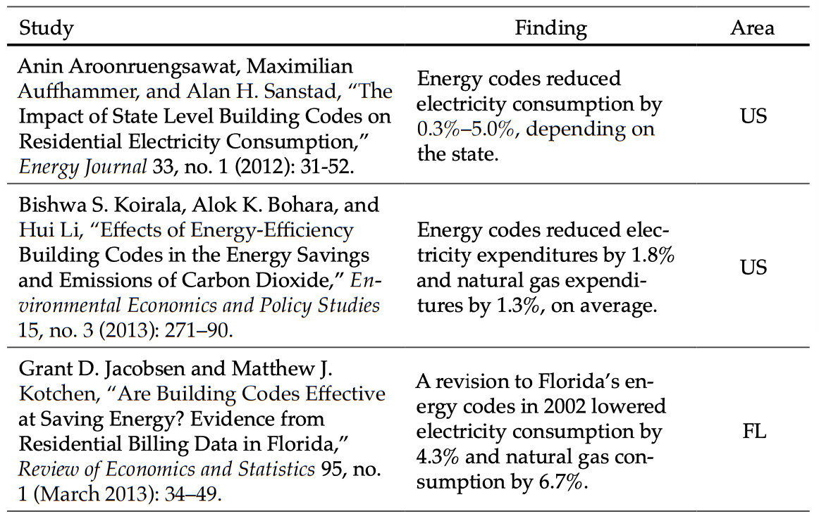
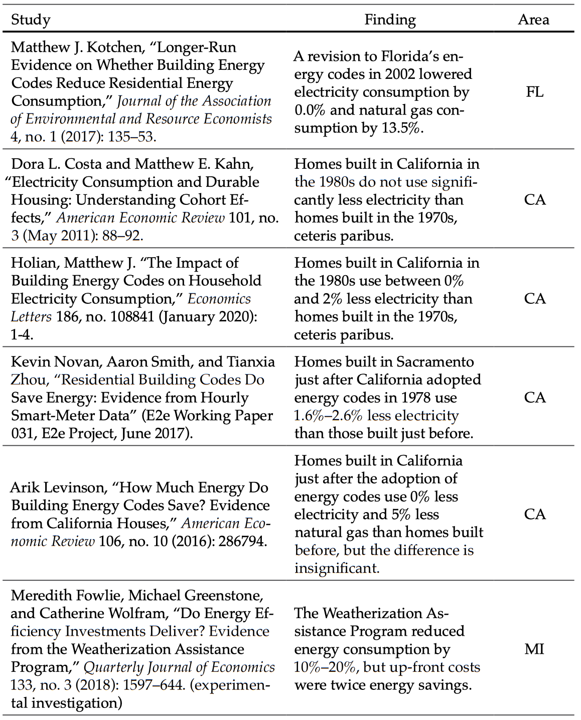
Note: These nine studies use various methods to estimate the impact of energy codes on energy use.

References