Sanctuary Cities and Crime

Otsu, Yuki

1 Introduction

Sanctuary policies have gained more attention in recent policy debates. Although there is no single definition of a sanctuary city, it is generally considered to be a city that does not cooperate with the federal government in terms of immigration policies.¹ In debates about immigration policies, sanctuary cities are often mentioned in the context of the safety of communities. One perspective says that sanctuary policies could raise crime. The U.S. Department of Homeland Security (2018) described sanctuary cities as follows:

Non-cooperative jurisdictions that do not honor U.S. Immigration and Customs (ICE) detainer requests to hold criminal aliens who are already in their custody, endanger the public and threaten officer safety by releasing criminal aliens back into the community to re-offend. In addition to causing preventable crimes, this creates another “pull factor” that increases illegal immigration.

This statement points out that sanctuary policies release criminal aliens to the communities and make the city more attractive to illegal immigrants.
However, another perspective says that sanctuary policies do not raise the crime rate, and it could even decrease crimes. The predominant reason to implement a sanctuary policy is to encourage undocumented immigrants to report incidents when they become witnesses or victims. As the International Association of Chiefs of Police (2004) said,

Many law enforcement executives believe that state and local law enforcement should not be involved in the enforcement of civil immigration laws since such involvement would likely have a chilling effect on both legal and illegal aliens reporting criminal activity or assisting police in criminal investigations. They believe that this lack of cooperation could diminish the ability of law enforcement agencies to effectively police their communities and protect the public they serve.

A simple comparison between sanctuary and non-sanctuary cities may be misleading since sanctuary and non-sanctuary cities are different in various respects. The previous literature on sanctuary policies found that sanctuary cities are associated with low crime rates (Martínez-Schuldt and Martínez, 2019; Martínez et al., 2018). However, we know little about the causal effect of sanctuary policies on crime rates.

This paper investigates whether the adoption of sanctuary policies causes a change in crime rates for a city. So far, the literature lacks two things. First, the literature does not control for heterogenous trends in crime rates across geographic areas. For instance, California has more sanctuary cities, but the crime rate in that state is also declining. We need analyses to avoid simply capturing a trend specific to the states that have more sanctuary cities. Second, the literature is relatively silent about crime type heterogeneity. The empirical papers about sanctuary policies focus only on one or two types of crime, such as homicide and robbery, and it remains unknown if the findings hold for other crimes.

For causal inference, I construct panel data of U.S. cities from 1999 to 2010. Following the literature, sanctuary status is determined based on a list made by the National Immigration Law Center (NILC). Using data from the Uniform Crime Reports (UCR) from 1999 to 2010, this paper tracks how much crime rates change before and after the implementation of the policy. Then, with a difference-in-differences approach, I exploit the differential timing of the policy implementation across sanctuary cities to identify the causal effect of sanctuary policies on crime.

This paper finds that sanctuary policies do not cause an increase in violent crimes, but they do decrease property crimes somewhat. The results are robust to controls for the efficiency of the local government and other immigration policies, although results using a matching DID methodology do not show any effect of sanctuary policies on crime. The paper then tests for whether sanctuary policies attract immigrants to a city. Sanctuary policies do not appear to increase the fraction of foreigners, migrants (including domestic migrants), and likely undocumented Mexican immigrants. Hence, the sanctuary policy does not seem to attract immigrants.

Finally, this paper also performs an event study to check the pre-trend and the heterogeneity of the policy effect over time. The event study shows that (a) there is no clear pre-trend before the adoption of sanctuary policies, and (b) crime rates show evident decreases starting from one year after the implementation. It is worth noting that neither the DID nor the event study results show a positive effect of sanctuary policies on local crime rates.

2 Background

The relationship between immigration and crime in the U.S. context has been investigated for a long time.² For example, immigrants overall are less likely to be committed to prison (Moehling and Piehl, 2009), and more immigrants in Metropolitan Statistical Area (MSA) lead to a lower crime rate (Reid et al., 2005). Looking specifically at Mexican immigrants, Chalfin (2015) used a network instrumental variable and found negative impacts of Mexican immigrants on rape and larceny rates at MSA level and a positive impact on assault. Light and Miller (2018) focused on undocumented immigrants and, with a fixed-effect model, found a negative association between undocumented immigrants and violent crime at the state level. Ousey and Kubrin (2018) published a recent survey on the literature in sociology. They found that most of the papers find no relationship between immigration and crime, and even among papers that found a significant relationship, most of them found a negative relationship.Hence they concluded that the overall immigration-crime association is negative but weak.

Another literature focuses on the effects of immigration policies on crime (Baker, 2015; Freedman et al., 2018). Granting legal status of immigrants decreased property crime (Baker, 2015), but felony charges rose for those who had not gained legal status (Freedman et al., 2018).³

In terms of policy impacts on immigrants, Miles and Cox (2014) looked at whether a harsher policy against undocumented immigrants changes crime rates. In particular, they focused on the Secure Communities (SC) program, where fingerprint information collected by local police is automatically sent to the. Department of Homeland Security. Miles and Cox (2014) performed a difference-in-differences regression using a county-level variation of implementation timing and concluded that the SC program does not change crime rates. Although Miles and Cox (2014) found no impact on crime rates, Alsan and Yang (2018) found the SC program induces fear of deportation among Hispanics and decreases demand for safety net programs. Churchill et al. (2019) focused on E-Verify laws, which require employers to check if new employees are legally eligible to work. They found that E-Verify laws decreased property crimes involving Hispanic arrestees, likely because of more employment among low-skilled natives of Hispanic origin and outmigration of young
immigrants.

There are several papers investigating sanctuary cities and crime (Lyons et al., 2013; Wong, 2017; Martínez-Schuldt and Martínez, 2019; O’Brien et al., 2019). Martínez et al. (2018) summarized the recent contributions of the literature. So far, the literature has found evidence of null or negative relationships. Lyons et al. (2013) used data at the census tract level and found a strong negative relationship in sanctuary cities between violent crime and the concentration of immigrants in a neighborhood. Wong (2017) compared sanctuary and non-sanctuary cities using a matching method and found that crime rates are generally lower in a sanctuary city. O’Brien et al. (2019) conducted two types of analysis. They statistically tested if the passage of sanctuary policies changed crime rates within a city, and also checked whether there was a difference in crime rates between a group of sanctuary cities and a group of matched non-sanctuary cities. Their paper found no discernible difference in violent crime, rape, and property crime rates after the passage of sanctuary policies. Also, the matching results suggest that the sanctuary cities have no differences in crime rates compared to the non-sanctuary cities. Martínez-Schuldt and Martínez (2019) used an unconditional negative binomial model with city fixed effects to estimate the impact of sanctuary policies. They found that policy implementation is associated with the reduction of robbery, and they found no significant relationship with homicide. Taken all together, these papers found either no effect or negative effect on rates of various crimes. None of them found a positive effect on crime rates.

The approach in this paper is similar to Martínez-Schuldt and Martínez (2019), but there are two main differences. The first difference is an identification strategy. While Martínez-Schuldt and Martínez (2019) used an unconditional negative binomial (NB) regression with city fixed effects, I use a difference-in-differences (DID) approach based on a linear model. Osgood (2000) claimed that NB regression is superior to OLS regression when the city population is small, because a crime rate has a severe heteroskedasticity problem, and sometimes it is necessary to add an arbitrary constant to take the logarithm of the crime rate when it is zero. Although Martínez-Schuldt and Martínez (2019) followed the claim, I rely on OLS-based regression focusing on cities where the population is more than 100,000. Since the population is large and the number of crimes is also large, one unit increase in crime changes the crime rate almost continuously. Hence, heteroskedasticity is less problematic. Also, because I focus on large cities, crime counts take positive values in most of the sample cities. Summary statistics show a strictly positive number for all observations except homicide.

To control for time effects, Martínez-Schuldt and Martínez (2019) assumed linear and quadratic time trends common to all cities. However, as I show in Figure 1, although every crime rate decreases over time in their sample period, it sometimes shows kinks, and so linear and quadratic forms cannot capture the trend of crime rates well. Moreover, when the crime rates are divided by regions, they show a different time trend. Figure 2 shows the change in violent crimes by state from 1990 to 2014 (the number is normalized to the 2000 level). Although California and Illinois show a decreasing trend, Nevada, North Dakota, and South Dakota show an increasing trend. In 2014, North Dakota faced 274% more violent crime compared to the 2000 level, while Illinois faced 41% less. Hence, to evaluate the policy effect, we need to capture the geographically heterogeneous trends in crime rates. My paper uses a model with a city-specific linear time trend or state-year fixed effects, which are more flexible to capture the heterogeneous time trends. Lastly, Martínez-Schuldt and Martínez (2019) used a mean crime rate over three years as a dependent variable to smooth annual fluctuations. However, the policy effect is underestimated when there is an immediate effect from the year of implementation. This could be more problematic if the policy effects begin from the next year after implementation. The results of this paper show that the sanctuary policy has a lagged effect. Hence, it is likely that Martínez-Schuldt and Martínez (2019) underestimated the coefficients.

The second difference is in the details of the outcomes. For example, due to the reliability of the data, the literature focuses only on the effects on aggregated crime categories such as violent crime or property crime; analysis of subcategories is rare. Even when subcategories have been analyzed, they were limited to a specific type of crime, such as homicide, robbery, or rape. By focusing on subcategories, my method enables comprehensive analysis. First, since felony offenders are not covered by the sanctuary policy in many cities, the effects on felony and non-felony crimes may be different. Moreover, for the argument about immigrants and crime, property crime and its subcategories are important since property crime is more likely motivated by rational choices. The decision behind crimes of opportunity (such as theft) considers the gain from the crime and likelihood of apprehension, while violent crimes are more likely impulsive responses to frustration. Finally, since sanctuary policies may affect reporting behavior, reported crime rates could be higher even when the policy reduces the rate of crimes committed.

3 Theoretical prediction

This section briefly summarizes theoretical arguments about the effect of sanctuary policies on crime.⁴ When a policy changes at a city level, two things should be considered to interpret the effect on local crime rates: sorting and incentives. Both could affect local crime rates.

Sorting means that when a policy is implemented, the composition of the population could change through migration between cities. Sanctuary cities might attract undocumented immigrants from other cities, since they feel more safe in the sanctuary city. If undocumented immigrants have a different propensity for crime, then the local crime rate may change (Ousey and Kubrin, 2009). For instance, crime rates could fall if immigrants are less crime-prone (Butcher and Piehl, 2007; Tonry, 1997) than natives. Hence, the direction of the sorting effect is ambiguous and also depends on incentives.

Incentives arise from the cost and benefit of crime. In particular, sanctuary policies change the costs of crime. Becker (1968) explained that crime could be rational. From this perspective, an increase in the costs of crime would reduce crime. The expected cost of crime $c_{crime}$ consists of the probability of being caught $p_{caught}$ and the amount of sanctions $\delta_{sanction}$ : $c_{crime}=p_{caught} \times \delta_{sanction}$ . Sanctuary policies could affect each part, so the overall crime cost could go up or down. Sanctuary policies lower the sanction on undocumented immigrants when they commit a crime. Specifically, the punishment decreases because the local police do not begin the removal process. Undocumented immigrants no longer need to be concerned about deportation even when they are caught. For other people, the sanction of crimes does not seem to change because of a sanctuary city policy.

However, the expected cost of crime also depends on the probability of getting caught. The literature claims the probability could increase because of two reasons: a spiral of trust and informal social control. Lyons et al. (2013) referred to “a ‘spiral of trust’ that improves communication between officials and immigrants, promotes legislation protecting immigrant interests, and generates greater system-level trust in government.” Without a sanctuary policy, undocumented immigrants may not report a crime when they become victims or witnesses, because local police might discover their legal status, and deportation could happen. However, with such a policy, undocumented immigrants report more crime and trust the police. If sanctuary policies induce residents to trust police, then the police can get cooperation from residents and work more efficiently and effectively; eventually, the apprehension probability would increase.⁵ Also, the policy strengthens public social control, which arises from ties among residents. Buonanno et al. (2012) show that dense social interaction is associated with a lower rate of property crime. Moreover, informal public social controls are closely related to the relationship between residents and police. Using survey data in Chicago, Silver and Miller (2004) found that neighborhoods where people have more satisfaction with local police have a higher level of informal social control over delinquent behavior of youth. The probability of being caught will increase if residents strengthen informal social controls over crime. In summary, the change in the costs of crime is ambiguous, and it is hard to predict the sign of the policy effect from theory alone.

All the mechanisms so far are about committed crimes, but, in practice, we can only observe the reported crimes. Underreporting is common in crime issues. Sanctuary policies may induce residents to report more crimes, because the policies increase trust in police. Even if the number of committed crimes remains the same or decreases because of the sanctuary policy, the number of reported crimes could increase. Hence, we need to be cautious about the interpretation of the results. If the reported crime rate increases after the enactment of sanctuary policies, it could be either because of more committed crimes, less underreporting, or both. However, if we observe a decrease in the reported crime rates after the policies, it must be because the change in crimes committed dominates the effect of reduced underreporting.

4 Data & Approach

4.1 Deﬁnition of sanctuary city

There is no universally accepted definition of a sanctuary city. For example, Executive Order 13768, from 2017, defines sanctuary cities as “locales that refuse to comply with federal statute 8 U.S.C. 1373 enhancing information related to individuals’ immigration statuses with ICE or CBP.” Alternatively, the Department of Justice defines a sanctuary city as a “jurisdiction that may have state laws, local ordinances, or departmental policies limiting the role of local law enforcement agencies and officers in the enforcement of immigration laws.” There are also many lists of sanctuary cities, including the ones made by the Center for Immigration Studies (CIS)⁶and Ohio Jobs & Justice PACS (OJJPACS).⁷ Throughout this paper, the definition of a sanctuary policy is as follows: a sanctuary policy is a policy legislated by a local government that (1) inhibits the local enforcement agencies from cooperating with federal immigration authorities and (2) is stated explicitly in administrative documents such as resolutions, ordinances, executive orders, or police orders. A sanctuary city is a city that has any sanctuary policy. Note that this paper focuses only on the formal sanctuary cities. There are also informal sanctuary cities, which do not cooperate with federal authorities without having an explicit statement or policy. These cities are not counted as sanctuary cities since the definition of an informal sanctuary city is arbitrary to some extent.⁸ Following the literature (O’Brien et al., 2019; Martínez-Schuldt and Martínez, 2019), this paper uses a list of formal sanctuary cities offered by the National Immigration Law Center (NILC). There were 42 sanctuary cities in 2010.

The list by the NILC has some advantages over other lists. One is that there is a brief description of the policy for each city, which helps to identify the date of implementation and categorize its type of policy. However, one disadvantage is that the list was last updated in 2008. Following O’Brien et al. (2019) and Martínez et al. (2018), I checked each document and made a list of sanctuary cities (see Table 1).⁹¹⁰

For some cities in the list in Table 1, the actual year of implementation is different from that in the list by O’Brien et al. (2019). This is because these cities implemented a policy before the year, and reconfirmed or amended the policy later. I use the year when the policy was originally implemented. For example, the year of sanctuary status for San Francisco is set as 2002 in O’Brien et al. (2019), but San Francisco originally became a sanctuary city in 1989, and the policy was reaffirmed in 2002.

4.2 Data source

The data ranges from 1999 to 2010. The beginning year is set to 1999, because most of the sanctuary cities in the NILC list adopted their policies after 2000. I chose 2010 as the end period because Martínez-Schuldt and Martínez (2019) updated the list up to 2010 (the original list in the NILC was last updated in 2008). This extension gives a larger sample size for analysis. The list of sanctuary cities and the type of policies are summarized in Table 1.

Crime data is collected from the FBI Uniform Crime Reports (UCR). The data used for the analysis is annual, city-level, and reported. Categories of crime are violent crime (homicide, rape, robbery, aggravated assault) and property crime (burglary, larceny, auto theft).¹¹ The FBI also provides the number of police officers of each agency in the UCR,¹² and I use the number of sworn officers per capita.

To get demographic information for each city, this paper also uses data from the Census and the American Community Survey (ACS). The data is obtained from IPUMS for public use (Ruggles et al., 2019). Annual data is not available for all years, and so I use the 5% sample of the Census in 2000 and the annual sample of the ACS from 2005 to 2010. The data between 2000 and 2005 is filled by linear interpolation. The demographic analysis in Section 5.3 begins in the year 2000.

Sample cities satisfy the following two criteria: the population is larger than 100,000, and there are at least two observations during the sample period. To have as large a sample size as possible for the analysis and to do a more in-depth investigation, this paper uses two sets of samples: (1) the baseline sample and (2) the sample with time-variant characteristics. The baseline sample is made only from the UCR. Among all cities in the UCR data, 288 satisfy the two criteria, and there are 2981 observations in total.¹³ The sample with time-variant characteristics is constructed from the UCR and the ACS. Not all cities in the UCR are identified in the ACS, because the ACS Public Use data does not define all cities.¹⁴ The difference is mainly from dropping relatively small cities in terms of population and geographic size. As a result of merging the UCR and the ACS, the total sample size is 170 cities (including 35 sanctuary cities) and 1749 city-year observations.¹⁵

4.3 Regression model

The regression is based on a difference-in-differences approach. Specifically, I use the following specification:

(1) $\begin{equation*} \log y_{it}=\alpha_{sanc} Sanctuary_{it}+\alpha_X X+\eta_{i}+\eta_{t}+\gamma_{i} t+\epsilon_{it}. \end{equation*}$

The outcome variable $y_{it}$ is the crime rate of city $i$ at year $t$ , which is the number of reported crimes per 100,000 people in the city. I use a natural logarithm of the crime rate as a dependent variable. Both violent and property crime rates and each subcategory are analyzed. $Sanctuary_{it}$ is a binary variable that indicates the sanctuary status of city $i$ at year $t$ . Its value is one after the year of policy implementation. $\eta_{i}$ and $\eta_{t}$ are city and time fixed effects, respectively. $\gamma_i$ captures city-specific linear time trends. The regression coefficient of interest is $\alpha_{sanc}$ and the coefficient is the difference-in-differences estimates of the effect of sanctuary policies. Since the dependent variable is log of crime rates, $\alpha_{sanc}$ is the percentage change in crime rates due to the sanctuary policy. The regressions are weighted by city population, and standard errors are clustered at the city level.

Table 2 and 3 show summary statistics of the baseline sample and the sample with time-variant characteristics. In Table 2, violent crime consists of homicide, rape, robbery, and assault, and more than half of the violent crime rate is from assault. As for property crime, among three subcategories (burglary, larceny, and auto theft), larceny occupies more than half of the total. Table 3 shows summary statistics for the sample with time-variant characteristics. In the 170 sample cities, there are 35 sanctuary cities. Among the three types of policies, the most popular type is the don’t enforce policy, and its share is about half of the total observations. The don’t ask policy follows and the don’t tell policy is the least popular. The sum of the means of the three types is not equal to the mean of Sanctuary city, since some policies fall into multiple categories.

Figure 1 shows the mean of crime rates for both sanctuary and non-sanctuary cities with 95% confidence interval. In Figure 1, a group of sanctuary cities is defined by their status in 2010, hence, for the early years, the group of sanctuary cities contains cities that do not have the policy yet. Point estimates in the figure indicate that the violent crime rate is higher in sanctuary cities, and that is true for each subcategory except forcible rape. However, sanctuary cities have a lower property crime rate except for the auto theft rate, which does not show a significant difference between sanctuary and non-sanctuary cities. Overall, both sanctuary and non-sanctuary cities show a similar trend of crime rates, but not all the trends for each subcategory of crime are monotone.

4.4 Identiﬁcation

The DID estimator gives the average treatment effect on the treated (ATT). Identification relies on a change of sanctuary status and the different timing of the policy implementation. The different timing is summarized in Table 1. The number of sanctuary cities has increased over time. At the beginning of 1999, 9 cities (Austin, Chicago, Cleveland, Houston, Jersey City, Los Angeles, Salem, San Francisco, and Washington D.C.) were formal sanctuary cities. The number increased to 29 by 2005, and all 42 cities in the list employed at least one type of sanctuary policy by the end of 2008. Note that no city abolished its sanctuary policy in the sample period.

The DID approach requires a parallel trend assumption for identification of ATT: both treatment and control groups have the same time trend before and after the treatment. This paper assumes the parallel trend and argues the validity of the assumption by an event study in Section 6.

5 Results

5.1 Main results

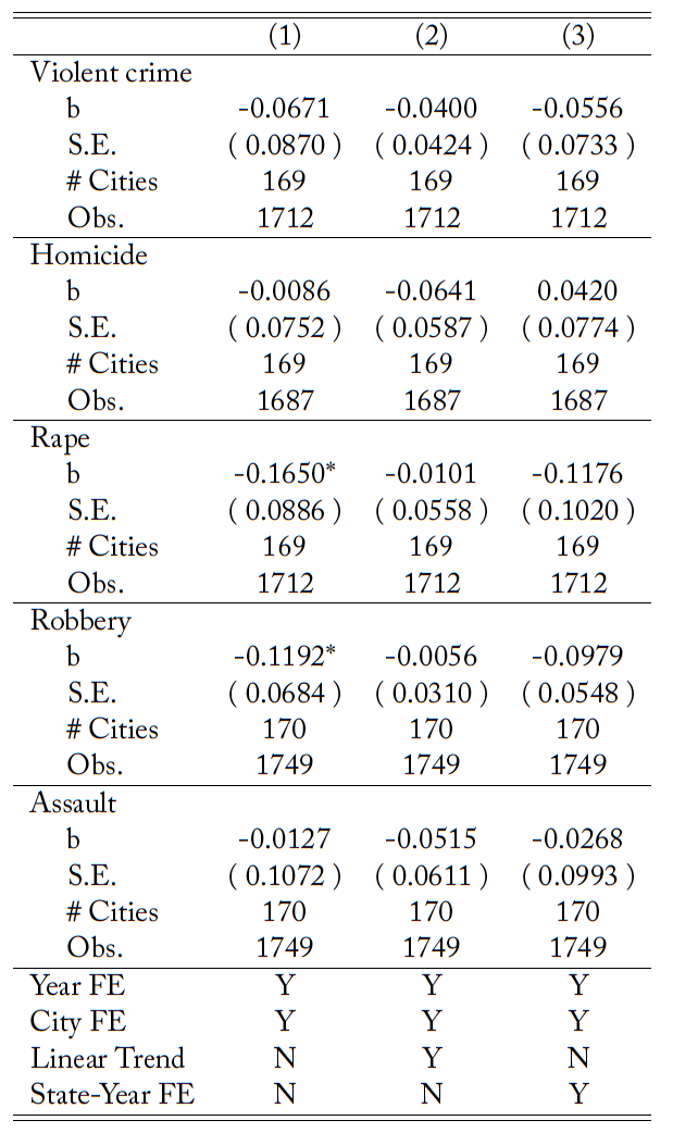
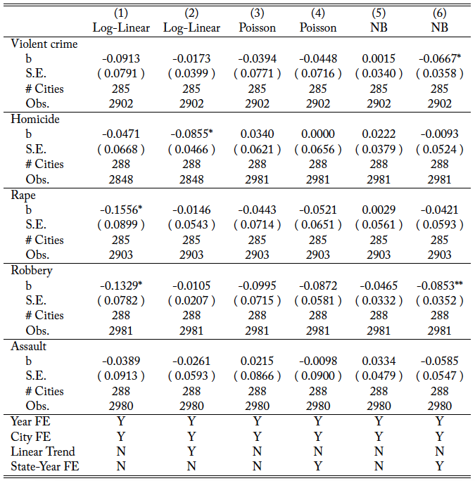
Baseline results are summarized in Table 4 and 5. Table 4 and 5 have three columns for each specification, and each b shows the effect of sanctuary policies on the crime type. The first column is the regression result with city and year fixed effects as well as the post-implementation dummy, but other covariates are not included. The result shows a negative effect on violent crime as a broad category. The violent crime rate decreases by 8% compared to the rate before the sanctuary policy, but the coefficient is statistically insignificant. All subcategories have negative coefficients, but none of them show a statistically significant decrease at the 5% level.

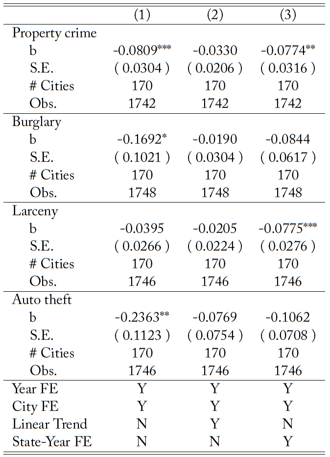
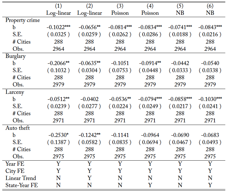
Table 5 shows that sanctuary policies lead to a decrease in the property crime rate by 9.2%. For subcategories, the coefficients show negative signs, but none of them show significance at the 5% level. The burglary rate declines 18.7%, and the larceny rate declines 4.5 percent compared to the crime rates before the sanctuary policy. The effect on the auto theft rate is negative but insignificant.

The second column controls for the city-specific linear time trend; this is the preferred specification. Most of the point estimates become small in an absolute sense, but this change reduces the standard errors of the estimates as well. As a result, the property crime rate still shows a significant difference induced by the policy and decreases by 6.3%. The homicide rate decreases by 8.3%, a larger effect than the estimator without trend terms.

Finally, the third column controls for the time trend as state-year dummies instead of linear trends. The state-year dummies cause the effects on the property crime and auto theft rates to vanish but make the larceny rate significant. The property crime rate shows a similar effect in terms of magnitude, but the standard error is relatively high. The auto theft rate becomes insignificant due to a smaller point estimate and the high standard error.

The baseline results show negative coefficients in general, but most of them are not statistically significant. However, although the effects on subcategories are not evident, the sanctuary policy leads to a significant decrease in property crime by 6.3%. Moreover, the point estimates and the standard errors give the upper bounds of the magnitude. In the worst case within the 95% confidence interval, the rape rate increases by 9%, but all other crimes can have at most 5% increases.

In summary, a sanctuary policy seems to have a negative effect on the general category of property crime in both samples, and some subcategories also show a negative effect. The results for homicide and robbery imply no effect of the policy, while Martínez-Schuldt and Martínez (2019) found no effect on homicide but a negative effect on robbery. A sanctuary policy also seems to reduce some of the remaining categories of crime not analyzed by Martínez-Schuldt and Martínez (2019).

5.2 Robustness checks

This section argues the robustness of the main results. Specifically, I consider several endogeneity issues. To check the possibility of self-selection bias, I also perform a matching DID in Appendix A. Alternative model specifications and other immigration policies are also considered in the
Appendix.

One concern about the main result is that the negative effects on the crime rate in sanctuary cities may come from better enforcement operations. In other words, the reduction may not be because of the sanctuary policies but because efficient governments induce lower crime rates as well as the adoption of sanctuary policies. To explore this possibility, I use two measures of the efficiency of local governments—government expenditure on education and interest payments for municipal bonds—as a control variable. Adding this variable as an additional control mitigates the endogeneity issue resulting from better operation of government. First, an efficient government would have better school quality. Since public schools rely primarily on local governments for their budgets, education expenditure is a good measure of school quality. I assume that expenditure on education is unrelated to crimes, at least in the short run,¹⁶ but is related to the efficiency of governments. Another measure is the interest payment for municipal bonds. The intuition is that, given the same amount of outstanding debt, an efficient government should pay less for the interest. In particular, I use the difference from the last year,

(2) $\begin{equation*} I_{it}=\frac{interest_{it}}{debt_{it}}-\frac{interest_{it-1}}{debt_{it-1}}, \end{equation*}$

where $debt_{it}$ is the amount of total outstanding debt in a city $i$ at time $t$ , and $interest_{it}$ is the interest payment for the outstanding debt at year $t$ . The expenditure and debt data are collected from the Annual Survey of State and Local Government Finances.

Table 6 summarizes the results. The results are similar to the baseline, but the magnitude of the effect is slightly larger. No clear effect is confirmed for violent crimes, although all the coefficients are negative. The point estimates imply that the property crime rate decreases by 6.8%. The subcategories of property crime show a similar coefficient, but most of them are statistically insignificant at the 5% level.

Another concern is reverse causality: a city government may employ a sanctuary policy because of high or low crime rates. Since one of the reasons why a city may enact a sanctuary policy is to encourage immigrants to report more information on crime, sanctuary policies may be a response to high crime. Alternatively, low-crime cities may enact sanctuary policies to keep crime rates low or to reduce them even further. To mitigate these possibilities, I perform the DID regression with matched samples based on the total crime rate as well as other covariates in 2000. The propensity-score matching enables a comparison of sanctuary cities and similar non-sanctuary cities. Limiting the sample cities on the common support gives the DID estimator that is more robust to the self-selection bias. The detailed method is in Appendix A.

The regression results in Table 7 imply that the sanctuary policy induces no difference. Most of the point estimates indicate the crime rates change by plus/minus 3%, and none of them are statistically different from zero. Hence, self-selection might cause the negative effect of the policy in the main result. However, none of the results show a positive point estimate that is significantly different from zero under the matching DID.

5.3 Why do sanctuary policies lead to lower crime rates?

The main results show that sanctuary policies lead to a decrease in crime rates for some categories. Section 3 explained the potential reasons why sanctuary policies affect crime rates: sorting and incentives. To explain the lower crime rates associated with sanctuary policies, I now investigate two possible channels: composition change of population and change in size of police force. If sorting is the reason for lower crime rates, that would mean sanctuary policies change the composition of city populations. As for incentives, Section 3 explains that sanctuary policies are expected to improve police operations through a spiral of trust. However, the sanctuary policy could reduce crimes without the spiral of trust if it also increases the size of the police force. In this section, I check how much the population composition and the police force size change depending on the policy.

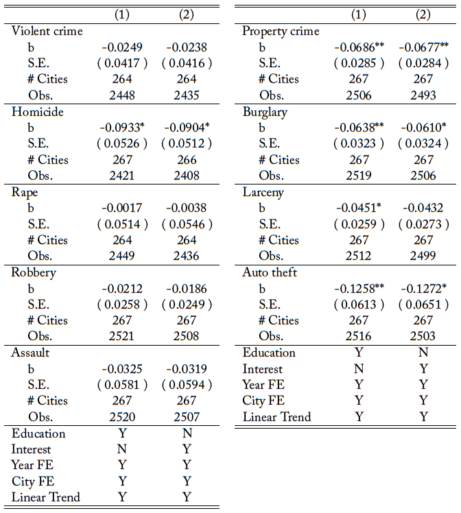
To investigate the effect on population composition, the UCR data is merged with the ACS data. Hence, this section uses the subsample of the main analysis.¹⁷ Since the sample is different from the main analysis, I check the DID results with the subsample. Table 8 and 9 show the results with time-variant characteristics. Each column is the same specification as in Table 4 and 5. Because of this sample selection, the significance of coefficients changes for property crime. Property crime still shows a negatively significant effect in the model without linear trends but becomes insignificant with linear trends. The coefficients for auto theft become insignificant. The estimated coefficient is smaller than that of the baseline result. The coefficient on the rape rate is 2%, which is larger (in the absolute value) than the baseline result (1%). The point estimate for the robbery rate is less than 1%. The effect on property crime is smaller than the result in the previous section. Overall, although some coefficients change the statistical significance, the subsample analysis gives similar results.

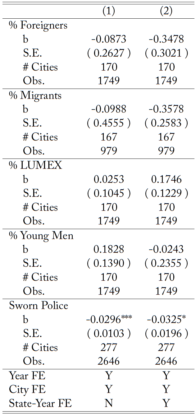
First, to check demographic changes caused by the sanctuary policy, I run a regression of different demographic groups’ population percentages in Table 10. The dependent variable is the percent of the demographic group in the city and so ranges from 0 to 100. The interpretation of the coefficient is the percentage point change for that demographic group. The results in Table 10 show a modest decrease in the fraction of foreigners, but the coefficients are not significant at the 5% level. The second row in Table 10 shows the result for those who migrate from other states to the city in the past year. Although the estimated coefficients show a negative impact, the fraction does not change significantly before and after the implementation of sanctuary policies. The third row uses likely undocumented Mexican immigrants (LUMEX) as a dependent variable. The definition of LUMEX is based on Hall and Stringfield (2014). They define LUMEX as a group of immigrants from Mexico who (1) are non-citizens, (2) are not current students, (3) do not have some college or a higher degree, (4) do not work in the government sector, and (5) arrived to the U.S. after 1990. The results show no evidence that LUMEX responds to the sanctuary policy. A sanctuary policy may also change the share of young men, which are the main crime-prone group. However, the estimated result in the fourth row shows no discernible effect on the share of young men. So, overall, demographic changes are unlikely to be the reason for the crime rate changes.

Next, the last rows in Table 10 check if changes in the police forces caused the apparent effects of sanctuary policies on crime rates. Crime rates would drop if the implementation of the sanctuary policy happened alongside an increase in the police force. To check this channel, I regress the log of the number of sworn officers per capita as a dependent variable. The results show a significant negative effect of the policy. The sanctuary policy reduces per-capita sworn officers by 3%. In contrast to the initial expectation, the size of the police force is not increased by sanctuary policies, and hence the police force is unlikely to be the reason for the negative effect on crime rates.

In summary, at least, there is no evident increase in foreigners, migrants, or the size of the police force in sanctuary cities. Hence, I conclude that a decrease in crime rates is not likely due to sorting or an increase in the police force.

6 Event study

The DID results are informative about the effect of the sanctuary policies. For further investigation, this section performs an event study. Specifically, there are two reasons to do the event study analysis.

First, an event study design enables us to confirm the existence of the pre-trend. For the DID estimators to be valid, this paper assumes that the time trends between treatment and control groups are parallel. If the parallel trend assumption fails, then DID estimators are likely to contain the effects of other factors. For example, the anticipation of policy implementation could change the behavior of people even before the date of the policy implementation. Cities may start an informal sanctuary policy gradually and then make it as a formal policy at a later point.

Second, an event study can show the heterogeneity of the policy effect. Residents in a city might need time to learn about sanctuary policies and might forget the existence of the policies if the city became sanctuary a long time ago. However, the DID coefficients cannot capture the heterogeneous effects over time.

Let $k$ be the relative event date (year). The policy is activated at $k=0$ . The following specification is used:

(3) $\begin{equation*} \log y_{it}=\sum_{k=-3, k\neq -1}^{3}\alpha_{k} \times \mathbb{1}(t=t^{activation}_{i}+k)+\eta_{i}+\eta_{st}+\epsilon_{it} \end{equation*}$

where $t_{i}^{activation}$ is the year of policy adoption in a city $i$ . Regardless of the value of $k$ , $\mathbb{1}(t=t^{activation}_{i}+k)=0$ for non-sanctuary cities. I set $k=-1$ as the base year for sanctuary cities, which is one year before the implementation year. $\eta_{st}$ are state-year dummies to control state-specific time-trends. Since the time span is not long and there are few observations at the extreme, $k=3$ $(k=-3)$ includes any city-year observation that passed the policy more than 3 years before (after). The estimated coefficients $\alpha_{k}$ are summarized in Figure 3 and 4, and Table 11.

To begin with, Figure 3 tells if there is a trend before the sanctuary policy. Among violent crimes, the crime rates do not show significant differences except homicide before the policy implementation. The homicide rate is significantly lower only at three years before the policy implementation. For property crime and its subcategories, the coefficients before the policy are similar and not statistically different from zero. Hence, I conclude that there is no clear pre-trend, although it may be the case that a higher homicide rate induces a city to adopt a sanctuary policy.

For the violent crime rates, as shown in Figure 3, the coefficient in the year of the policy implementation is not different from zero, but it declines from the following year. The coefficient at 3 years after shows 12% less violent crimes and is significant at the 5% level. For the subcategories, the point estimates do not show a significant difference within the year of implementation. Estimated coefficients for homicide and rape show no clear pattern, although both have negative point estimates at time 3. Robbery and assault show persistent effects over three years after the implementation. The robbery rate shows a clear difference at time 3: the rate is 15% lower than the year prior to the implementation.

Compared to violent crime, the effects on the property crime rate are more clear. The estimated coefficient at the year of implementation is slightly negative but not significantly different from the prior year. The coefficients become negative from one year after the implementation and statistically significant up to three years after. The property crime rate is 8–12% less than at time -1 for those years. Among subcategories, the burglary rate shows a significant decrease in the first and third years after the implementation but not for the second year. The coefficients for the larceny rate slightly decrease at time zero, and decrease gradually after that. The coefficients for the auto theft rate show a negative effect of the sanctuary policy, and the effect is gradually strengthened over three years. The auto theft rate is 5.6% lower at the year of implementation and 22% lower at three years after.

Figure 4 is the same set of graphs for the sample with the ACS data. Overall, the event study results are very similar to the results of the baseline sample.

The event study results suggest that there is a clear pattern for property crimes but not for violent crimes. For property crimes, the effect becomes evident from one year after the policy adoption, and the size of the effect is similar in the following year. The coefficients up to 2 years later seem to show an increasing effect of the policy. However, further investigation is needed since the time length for the analysis is so limited.

7 Discussion

The results of this paper indicate that a sanctuary policy has a negative effect on property crime, and some subcategories also show a negative effect. The results for homicide and robbery imply no effect of the policy, while Martínez-Schuldt and Martínez (2019) found no effect on homicide but a negative effect on robbery. In the Appendix, the negative binomial regression confirms the negative effect of the policy. However, I could not find a significant effect on robbery in any other specifications. Hence, the effect on a robbery rate may be weak.

This paper considers two reasons why a sanctuary policy could change crime rates: sorting and incentives. The results do not show that sanctuary policies cause any change in the proportions of foreigners or migrants, so this paper found no evidence of sorting. Hence, the reduction of crime is likely from the lower propensity to commit crimes rather than compositional change. This paper cannot identify the reason why the propensity changes, but the results are compatible with the spiral of trust and informal social control stories. For future direction, it would be helpful to understand which groups (natives, legal immigrants, and undocumented immigrants) are affected by the policy. The policy discussion on this topic has mainly been concerned with undocumented immigrants. However, the sanctuary policy could change the costs of crime for natives and legal immigrants as well, because police operations seem to become more efficient because of the spiral of trust and informal social control.

A sanctuary policy may affect the reporting of crimes, so decomposing the effect into criminal behavior and reporting behavior would be helpful. So far, most of the results show no discernible effect. However, it is not clear if the sanctuary policy has no impact on any behavior, or if the sanctuary policy affects both criminal and reporting behaviors but they cancel each other out.

8 Conclusion

This paper investigates whether sanctuary policies cause an increase in crime, using a city-level variation of implementation timing from 1999 to 2010. The results show that sanctuary policies do not cause an increase in crime. Instead, sanctuary policies lead to a decrease in the property crime rate. The regression results using the sample with time-variant characteristics show no effect of the policy, and the robustness checks make some effects insignificant. Hence, the negative effects are not robust for any crime category, although the property crime rate shows a negative effect in most specifications.

What is consistent across the regressions is that none of the results show a positive association between sanctuary policies and local crime rates. In the event study design, sanctuary policies lead to decreases in robbery, property crime, burglary, and auto theft rates, and the effects start one year after implementation. Moreover, the policy does not lead to an increase in the proportion of foreigners or migrants, so sorting is unlikely to be the source of a decrease in crime rates.

Appendices

A Matching DID

To evaluate the effect of sanctuary policies, the treatment and control groups should be similar. However, sanctuary cities and non-sanctuary cities have different demographic characteristics as O’Brien et al. (2019) pointed out.¹⁸ Since sanctuary status is an outcome of choice by a local government, the local government might self-select the status; the self-selection causes a bias for the estimates. To check the bias, I perform DID regression with matched samples. The method in this section is based on Heckman et al. (1997). I match each sanctuary city based on its propensity score to be a sanctuary city by 2010. The city characteristics in 2000 are used for the propensity-score matching and so I drop nine cities that started a sanctuary policy before 2000. To compute the propensity scores, the following variables are used: (1) log of population, (2) % female, (3) % age groups (15–29, 30–44, 45–59, 60 or above), (4) % racial groups (Black, Asian, Pacific Islander, Native American, Other race), (5) % Hispanic, (6) % less than high school degree, (7) % college or above degree, (8) poverty rate, (9)% unemployed, and (10) the sum of the violent and property crime rates. The matching method is the Epanechnikov kernel matching on the common support.¹⁹

After the propensity-score matching, the estimation uses 136 cities (including 14 sanctuary cities) and 1464 observations. Figure 5 confirms that the matching method reduces the difference between the treated and control groups. Table 12 indicates the treated and control groups have no statistical difference after matching in terms of observables.

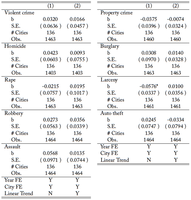
The regression results in Table 7 show an insignificant effect on property crime and violent crime. As a subcategory, larceny shows a significant negative effect at the 10% level. However, none of the coefficients shows a discernible effect of sanctuary policies once the city-specific time trend is controlled for. The coefficient for larceny thefts has a positive coefficient but it is statistically insignificant.

Although the point estimates are insignificant, all the estimates show a relatively small effect of the sanctuary policy. The point estimate for robbery indicates an increase of 3.6% but it is only slightly above one standard deviation. The estimator for auto theft indicates a 3.3% decrease with high standard errors.
In summary, sanctuary policies may have negative effects on some categories of crime, but the effects are not clear under the matched sample; the level of significance changes, in particular, for property crimes. However, both the baseline and matching results provide no evidence that sanctuary policies increase crimes.

Robustness Checks

B.1 Count data

Instead of the log of crime rates, this section uses the counts of each crime as a dependent variable. Table 13 and Table 14 use the log of crime count as the dependent variable, and the log of the population is added as an additional covariate. The results are similar to the main results but the coefficients have larger point estimates. For example, the effect on the burglary rate is −5.9% in the main regression, but the log of counts regression indicates −6.4%, which is statistically different from zero at the 5% level.

Table 13 and Table 14 show the results of Poisson and negative binomial (NB) regression results. In terms of statistical significance, both Poisson and NB give similar results except for robbery. Under the Poisson model, the sanctuary policy has no effect on robbery, but the NB model with linear trends supports a negative effect of sanctuary policies. Since the standard errors for each crime are high relative to the mean in the summary table, there is an overdispersion problem. Hence, the NB model would be appropriate. The estimator in the NB model −.0853 is interpreted as the robbery rate being 8.2% (= 1 − exp(−.0853)) lower after the adoption of sanctuary policy.

B.2 Other immigration policies

This section considers county-level or state-level immigration policies. Especially, state-level or county-level sanctuary policies, the Secure Communities (SC) program, and the 287(g) program.

B.2.1 State-level and county-level sanctuary policies

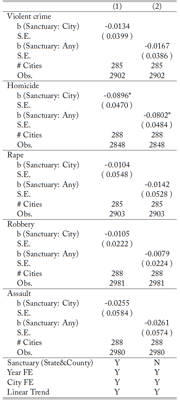
This paper performed city-level analysis, and the sanctuary status of a city is sorely based on the city policy. However, sanctuary policies can be adopted at the state or county level as well. (I call them upper-level policies.) Although the city police department deals with crime cases within a city, residents might care about the upper-level regulations. This section confirms the main result by controlling for the upper-level sanctuary policies. This section uses the list of sanctuary jurisdictions in NILC to define sanctuary states and counties. In the list, there are only 4 states and 7 counties identified as sanctuary jurisdictions.

I consider two ways to deal with upper-level sanctuary policies. The first way is that upper-level policies may have an additive impact on the effect of the city-level policy. In this case, the regression is performed with the upper-level sanctuary dummy, which takes a value of one when either the state or county adopts sanctuary policies. The second way is that cities in the jurisdiction may be considered as sanctuary cities whenever the state, county, or city adopts the policies. A city need not have its own sanctuary policies in this case to be a sanctuary city.

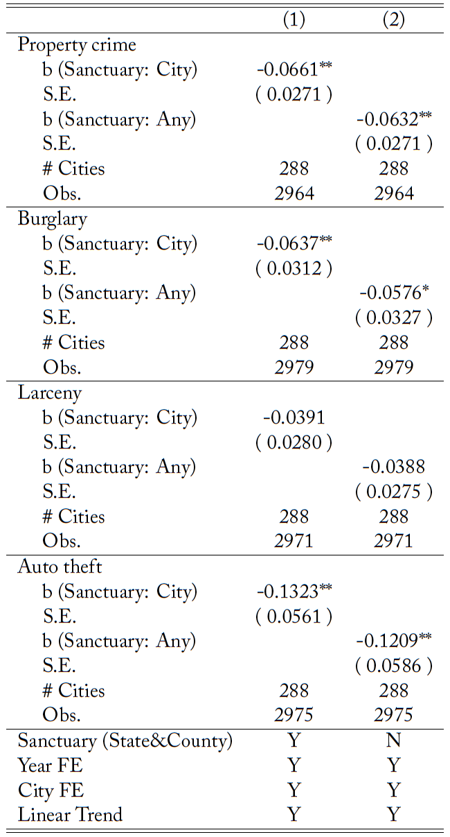
The regression results are in Table 15 and16. In the first column, upper-level sanctuary policies are controlled as additional dummy variables in the regression. Alternatively, the second column defines sanctuary status at any jurisdiction level. Compared with the main result, the two specifications show similar point estimates, and property crime and auto theft have statistically negative coefficients. For example, the estimator suggests that the property crime rate decreases by 6.3% if there is a sanctuary policy at any jurisdiction level.

B.2.2 Secure Communities program and 287(g) program

This section considers the two immigration policies adopted by local governments: the SC program and the 287(g) program. The two programs assist the federal government in enforcing immigration law. The SC program started in 14 jurisdictions in 2008, and all local jurisdictions participated in the SC program by January 22, 2013. Under the SC program, U.S. Immigration and Customs Enforcement (ICE) obtains the fingerprints of the county and state arrestees. The first 287(g) agreement was signed with the state of Florida in 2002, and 72 agreements were signed as of October, 2010 (Capps et al., 2011). Section 287(g) in the Immigration and Nationality Act enables local officers to enforce a part of federal immigration law, such as screening people and issuing detainers to hold them until the federal officers take custody.

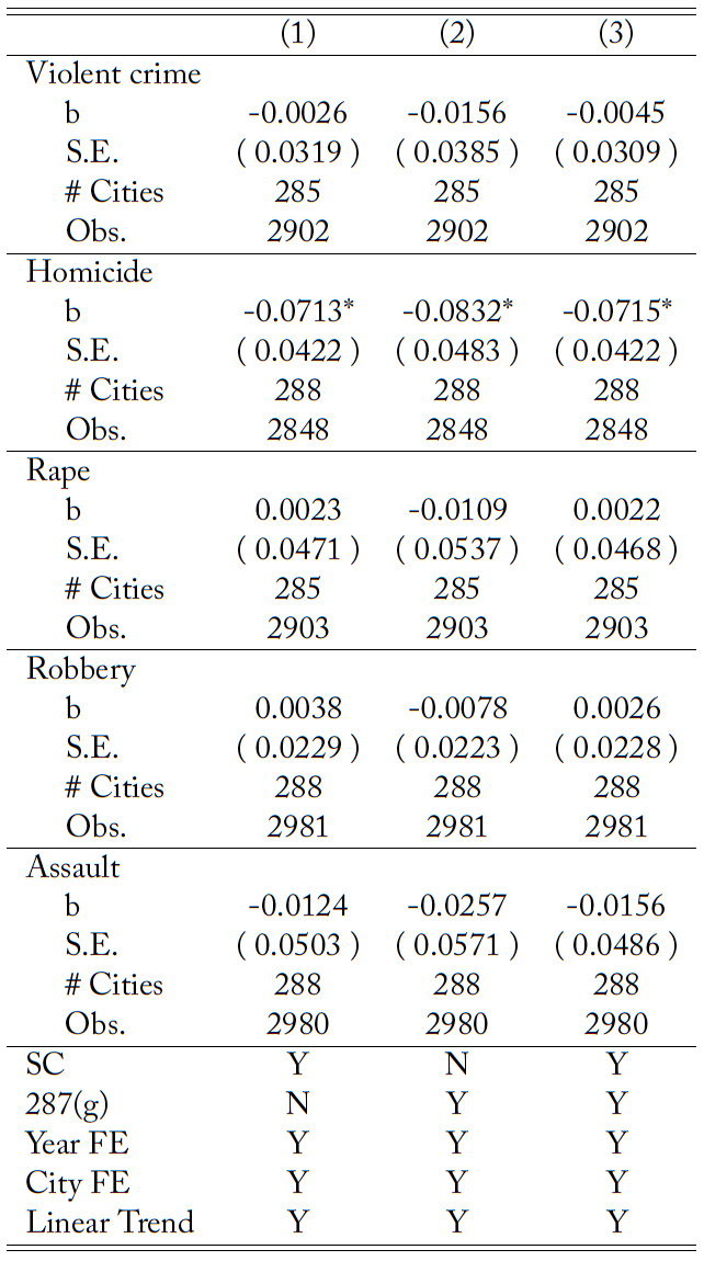
Table 17 and 18 summarize how these immigration policies change the main result. The table contains three columns: the result with (1) the SC dummy, (2) the 287(g) dummy, and (3) both the SC and 287(g) dummies. Overall, the estimated coefficients are similar, and the statistical significance of the estimators remains the same. For example, when both SC and 287(g) are controlled, the estimator suggests a 5.8% reduction of property crime, which is slightly lower than the estimator in the main result (6.3%). Since all sanctuary jurisdictions in the data passed the policy by 2008 and the SC program had started in 2008, the SC dummy partially captures the negative effect of sanctuary policies. The estimation results suggest that SC and 287(g) programs do not affect the estimators of sanctuary policies.

Figure 1. Crime rates by crime category and sanctuary status

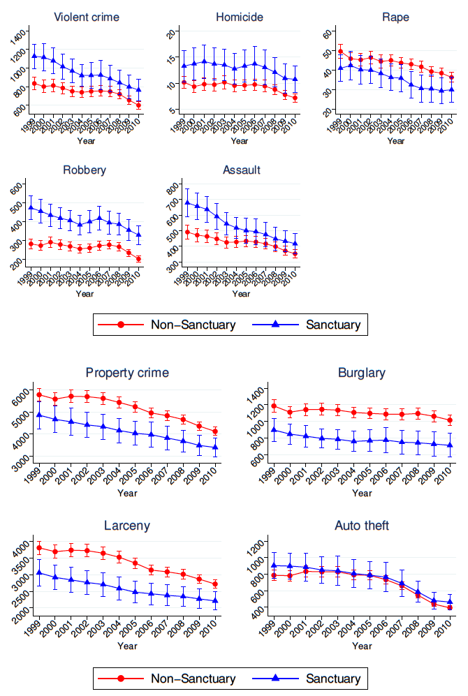
Note: Each graph shows the mean crime rate for both sanctuary and non-sanctuary cities with 95% confidence intervals. The crime rate is defined as the number of reported crimes per 100,000 population and weighted by city population. The group of sanctuary cities consists of every city where a sanctuary policy was adopted by 2010. Hence the composition of the two groups does not change over time. However, due to this definition, some of the “sanctuary” cities had not adopted the policy in the early years. The homicide rate in 2001 does not count the victims from the September 11 attacks. Cities in Illinois are treated as missing for the forcible rape rate since the definition of forcible rape used in Illinois does not comply with the UCR guidelines.

Figure 2. Violent crimes by state

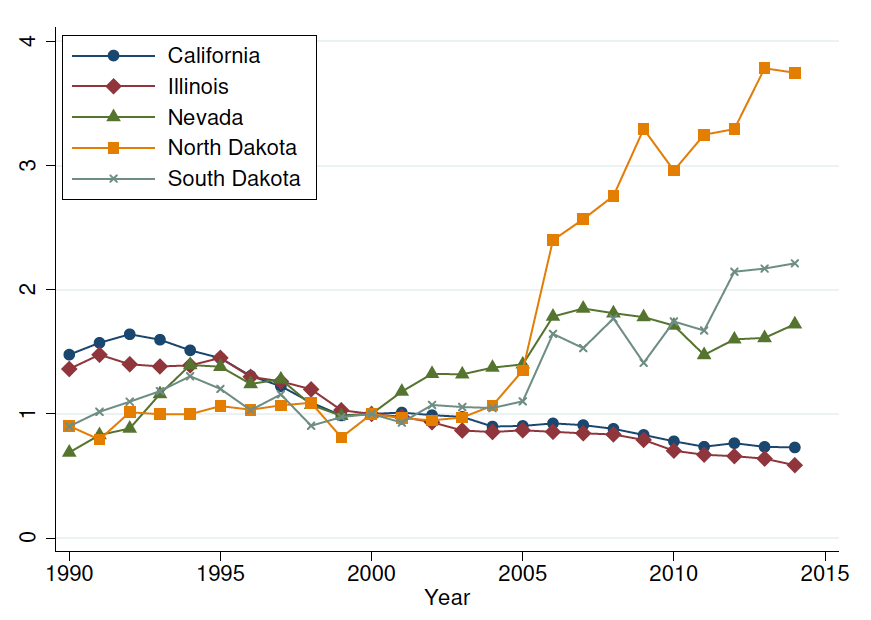
Source: UCR
Note: The level of violent crimes is normalized to the 2000 level in each state.

Table 1. List of sanctuary cities

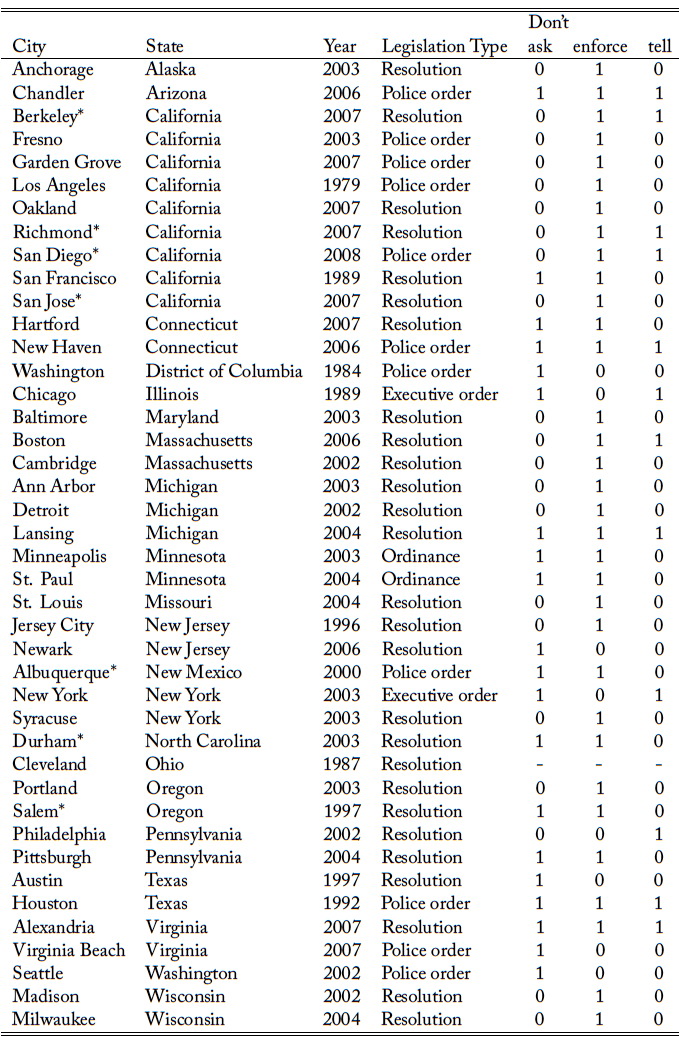
Note: All cities in the list have more than 100,000 population. Cities with * do not match the ACS data for public use in IPUMS and hence the cities appear in the baseline sample only.

Table 2. Summary statistics (baseline sample)

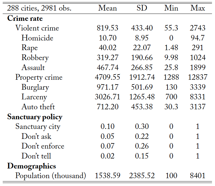
Note: The crime rate is defined as the number of reported crimes per 100,000 population. Crime rates and demographics are weighted by city population. “Sanctuary city” takes a value of one if an observation is after the sanctuary policy has employed. In total, there are 2969 observations, but there are some missing values in the UCR except homicide and robbery. The number of observations for each crime category is assault (2980), auto theft (2975), burglary (2979), larceny (2971), property (2964), rape (2903), and violent (2902).

Table 3. Summary statistics (sample with time-variant characteristics)

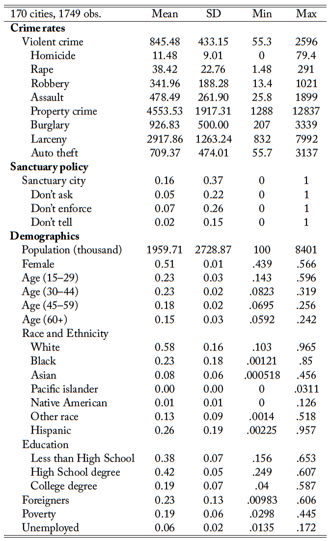
Note: The crime rate is defined as the number of reported crimes per 100,000 population. Crime rates and demographics are weighted by city population. Homicide and violent crime do not count the September 11 attacks. The sample period is from 2000 to 2010. Demographics in 2001–2004 are by linear interpolation of 2000 Census and 2005 ACS. The statistics are based on 170 cities and 1749 observations, but there are some missing values. The number of observations for each crime category is assault (1749), auto theft (1746), burglary (1748), homicide (1749), larceny (1746), property (1742), rape (1712), robbery (1749), and violent (1712).

Table 4. Baseline regression (violent crime)

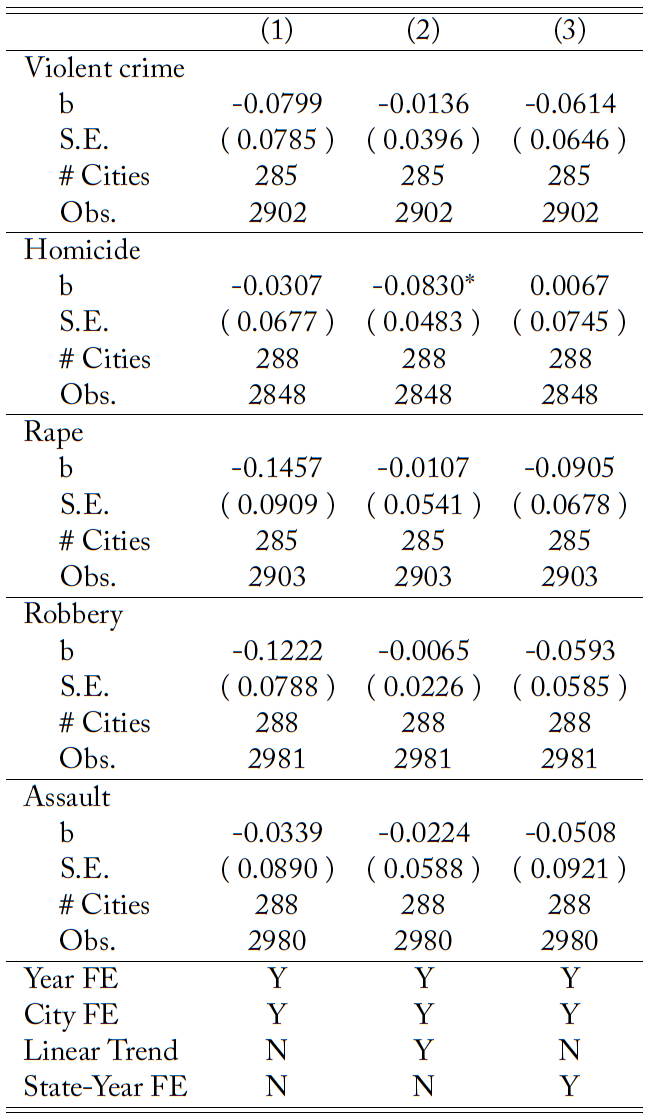
Robust standard errors in parentheses. *** p<0.01, ** p<0.05, * p<0.1.
Note: Dependent variables are log of crime rates. b is a coefficient

Table 5. Baseline regression (property crime)

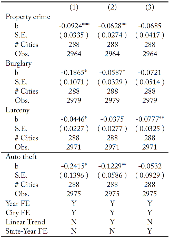
Robust standard errors in parentheses. *** p<0.01, ** p<0.05, * p<0.1.
Note: Dependent variables are log of crime rates.

Table 6. Regression with the expenditure on education and the interest payment for municipal bonds

Robust standard errors in parentheses. *** p<0.01, ** p<0.05, * p<0.1. Note: Education is city government expenditure on education per capita. Interest is the difference of the interest payment over total debt outstanding from the previous year. The data source for Education and Interest is the Annual Survey of State and Local Government Finances.

Table 7. Matching DID (kernel)

Robust standard errors in parentheses. *** p<0.01, ** p<0.05, * p<0.1.
Note: Linear trend is the city-specific trend.

Table 8. Baseline regression with the subsample (violent crime)

Robust standard errors in parentheses. *** p<0.01, ** p<0.05, * p<0.1.
Note: Linear trend is the city-specific trend. State-Year-FE is to capture state-specific time trend non-parametrically. The subsample is the cities in the UCR merged with the demographic information in the ACS.

Table 9. Baseline regression with the subsample (property crime)

Robust standard errors in parentheses. *** p<0.01, ** p<0.05, * p<0.1.
Note: Linear trend is the city-specific trend. State-Year-FE is to capture state-specific time trend non-parametrically. The subsample is the cities in the UCR merged with the demographic information in the ACS.

Table 10. Effects on other outcomes

Robust standard errors in parentheses. *** p<0.01, ** p<0.05, * p<0.1.
Note: Except “sworn police,” the dependent variables are the percentage of each group and so they range from 0 to 100. The coefficients indicate the percentage point change. % Migrants is the fraction of the population who moved to the city within a year. It is available from 2005 to 2010. % LUMEX is a fraction of likely undocumented Mexican immigrants. % Young male is the fraction of the population that are men ages 15-34. “Sworn Police” is the log of the number of sworn officers in the city per capita and is obtained from the UCR. The coefficient is the percentage change associated with the sanctuary policy. The number of observations is smaller than the main analysis since not all cities have their own police.

Figure 3. Event study coefficients (baseline sample)

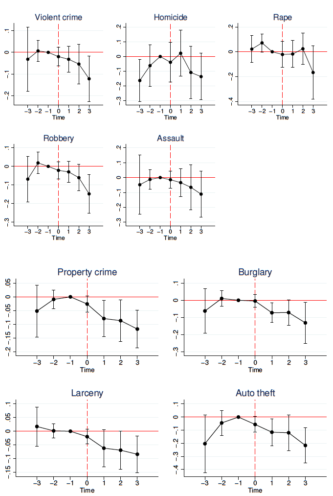
Note: All the graphs above use all observations for the baseline result. Each graph shows the event study coefficients with 95% confidence interval. Time 3 contains sanctuary cities that have implemented the policy more than 3 years ago and Time -3 contains sanctuary cities that will not until more than 3 years into the future. The base year is one year before the implementation.

Figure 4. Event study coefficients (sample with time-variant characteristics)

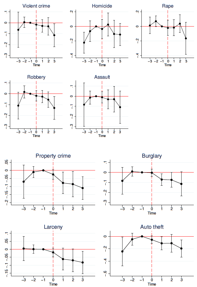
Note: All the graphs above use all cities with time-variant characteristics. Each graph shows the event study coefficients with 95% confidence interval. Time 3 contains sanctuary cities that have implemented the policy more than 3 years ago and Time -3 contains sanctuary cities that will not until more than 3 years into the future. The base year is one year before the implementation.

Table 11. Event study coefficients (baseline sample)

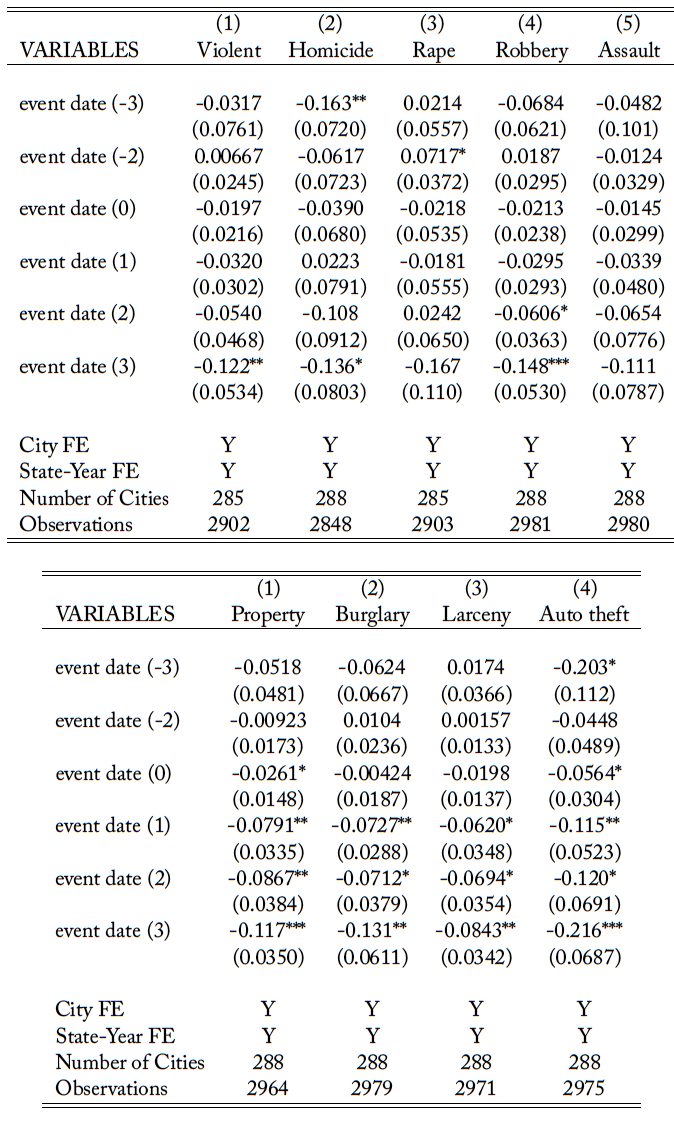
Robust standard errors in parentheses. *** p<0.01, ** p<0.05, * p<0.1.

Figure 5. Pre- and post-matching

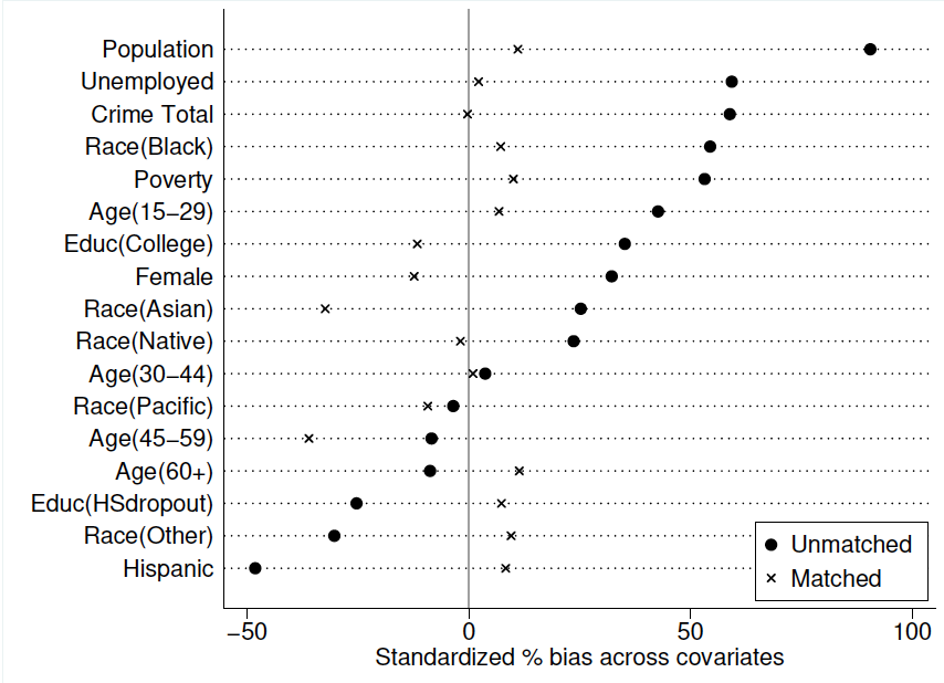
Note: Matching is based on the following characteristics: the sum of violent and property crime, log of population, female, age groups (15–29, 30–44, 45–59, 60 or above), racial groups (Black, Asian, Pacific Islander, Native American, Other race), Hispanic, less than high school degree, college or above degree, poverty rate, and unemployed.

Table 12. Post-matching comparison

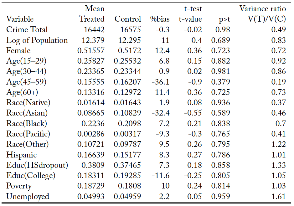
Table 13. Count data regression (violent crime)

Robust standard errors in parentheses. *** p<0.01, ** p<0.05, * p<0.1.
Note: Linear trend is the city-specific trend. State-Year-FE is to capture state-specific time trend non-parametrically.

Table 14. Count data regression (property crime)

Robust standard errors in parentheses. *** p<0.01, ** p<0.05, * p<0.1.
Note: Linear trend is the city-specific trend. State-Year-FE is to capture state-specific time trend non-parametrically.

Table 15. Sanctuary policies at state and county level (violent crime)

Robust standard errors in parentheses. *** p<0.01, ** p<0.05, * p<0.1.
Note: The sanctuary status of cities depends on the state, county, and city level. “b (Sanctuary: City)” is the coefficient for the sanctuary dummy at the city level that takes a value of one if the city itself adopts sanctuary policies. “b (Sanctuary: Any)” is the coefficient for the sanctuary dummy at any level that takes a value of one if the state, county, or city adopts sanctuary policies. “Sanctuary(State&County)” takes one if the state or county that contains the city adopts sanctuary policies. Linear trend is the city-specific trend.

Table 16. Sanctuary policies at state and county level (property crime)

Robust standard errors in parentheses. *** p<0.01, ** p<0.05, * p<0.1.
Note: The sanctuary status of cities depends on the state, county, and city level. “b (Sanctuary: City)” is the coefficient for the sanctuary dummy at the city level that takes a value of one if the city itself adopts sanctuary policies. “b (Sanctuary: Any)” is the coefficient for the sanctuary dummy at any level that takes a value of one if the state, county, or city adopts sanctuary policies. “Sanctuary(State&County)” takes one if the state or county that contains the city adopts sanctuary policies. Linear trend is the city-specific trend.

Table 17. Secure Communities and 287(g) (violent crime)

Robust standard errors in parentheses. *** p<0.01, ** p<0.05, * p<0.1.
Note: Dependent variables are log of crime rates. Linear trend is the city-specific trend.

Table 18. Secure Communities and 287(g) (property crime)

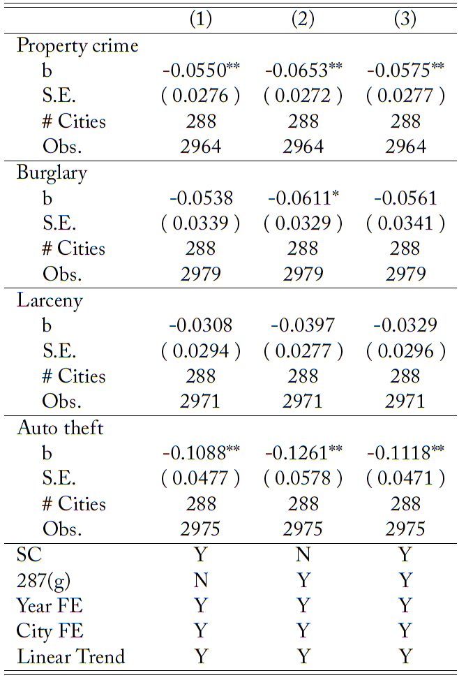
Robust standard errors in parentheses. *** p<0.01, ** p<0.05, * p<0.1. Note: Dependent variables are log of crime rates. Linear trend is the city-specific trend.

References

Alsan, M. and Yang, C. (2018). Fear and the Safety Net: Evidence from Secure Communities. SSRN Electronic Journal.

Baker, S. R. (2015). Effects of Immigrant Legalization on Crime. American Economic Review, 105(5):210–213.

Becker, G. S. (1968). Crime and Punishment: An Economic Approach. Journal of Political Economy, 76(2):169–217.

Bell, B., Fasani, F., and Machin, S. (2013). Crime and Immigration: Evidence from Large Immigrant Waves. Review of Economics and Statistics, 95(4):1278–1290.

Buonanno, P., Pasini, G., and Vanin, P. (2012). Crime and Social Sanction. Papers in Regional Science, 91(1):193–218.

Butcher, K. F. and Piehl, A. M. (2007). Why Are Immigrants’ Incarceration Rates so Low? Evidence on Selective Immigration, Deterrence, and Deportation. Working Paper 13229, National Bureau of Economic Research.

Capps, R., Rosenblum, M. R., Rodriguez, C., and Chishti, M. (2011). Delegation and Divergence: A Study of 287 (g) State and Local Immigration Enforcement. Washington, DC: Migration Policy Institute, 20.

Chalfin, A. (2015). The Long Run Effect of Mexican Immigration on Crime in US Cities: Evidence from Variation in Mexican Fertility Rates. American Economic Review, 105(5):220–225.

Churchill, B., Dickinson, A., Mackay, T., and Sabia, J. (2019). The Effect of E-Verify Laws on Crime. IZA Discussion Paper.

Freedman, M., Owens, E., and Bohn, S. (2018). Immigration, Employment Opportunities, and Criminal Behavior. American Economic Journal: Economic Policy, 10(2):117–151.

Hall, M. and Stringfield, J. (2014). Undocumented Migration and the Residential Segregation of Mexicans in New Destinations. Social Science Research, 47:61–78.

Heckman, J. J., Ichimura, H., and Todd, P. E. (1997). Matching As An Econometric Evaluation Estimator: Evidence from Evaluating a Job Training Programme. Review of Economic Studies, 64(4):605–654. International Association of Chiefs of Police (2004). Enforcing Immigration Law: The Role of State, Tribal and Local Law Enforcement. Technical report, The International Association of Chiefs of Police.

Kittrie, O. F. (2006). Federalism, Deportation, and Crime Victims Afraid to Call the Police. Iowa Law Review, 1(91):1449–1508.

Light, M. T. and Miller, T. (2018). Does Undocumented Immigration Increase Violent Crime? Criminology, 56(2):370–401.

Lochner, L. (2020). Education and Crime. In Bradley, S. and Green, C., editors, The Economics of Education, chapter 9, pages 109–117. Academic Press, second edition.

Lochner, L. and Moretti, E. (2004). The Effect of Education on Crime: Evidence from Prison Inmates, Arrests, and Self-Reports. American Economic Review, 94(1):155–189.

Lyons, C. J., Vélez, M. B., and Santoro, W. A. (2013). Neighborhood Immigration, Violence, and City-Level Immigrant Political Opportunities. American Sociological Review, 78(4):604–632.

Martínez, D. E., Martínez-Schuldt, R. D., and Cantor, G. (2018). Providing Sanctuary or Fostering Crime? A Review of the Research on “Sanctuary Cities” and Crime. Sociology Compass, 12(1):1–13.

Martínez-Schuldt, R. D. and Martínez, D. E. (2019). Sanctuary Policies and City-Level Incidents of Violence, 1990 to 2010. Justice Quarterly, 36(4):567–593.

Mastrobuoni, G. and Pinotti, P. (2015). Legal Status and the Criminal Activity of Immigrants. American Economic Journal: Applied Economics, 7(2):175–206.

Miles, T. J. and Cox, A. B. (2014). Does Immigration Enforcement Reduce Crime? Evidence from Secure Communities. Journal of Law and Economics, 57(4):937–973.

Moehling, C. and Piehl, A. M. (2009). Immigration, Crime, and Incarceration in Early Twentieth-Century America. Demography, 46(4):739–763.
National Immigration Law Center (2008). Laws, Resolutions and Policies Instituted Across the U.S. Limiting Enforcement of Immigration Laws by State and Local Authorities. Technical report, National Immigration Law Center.

O’Brien, B. G., Collingwood, L., and El-Khatib, S. O. (2019). The Politics of Refuge: Sanctuary Cities, Crime, and Undocumented Immigration. Urban Affairs Review, 55(1):3–40.

Osgood, D. W. (2000). Poisson-Based Regression Analysis of Aggregate Crime Rates. Journal of Quantitative Criminology, 16(1):21–43.

Ousey, G. C. and Kubrin, C. E. (2009). Exploring the Connection between Immigration and Violent Crime Rates in U.S. Cities, 1980–2000. Social Problems, 56(3):447–473.

Ousey, G. C. and Kubrin, C. E. (2018). Immigration and Crime: Assessing a Contentious Issue.
Annual Review of Criminology, 1(1):63–84.

Piopiunik, M. and Ruhose, J. (2017). Immigration, Regional Conditions, and Crime: Evidence from an Allocation Policy in Germany. European Economic Review, 92:258–282.

Reid, L. W., Weiss, H. E., Adelman, R. M., and Jaret, C. (2005). The Immigration-Crime Relationship: Evidence across US Metropolitan Areas. Social Science Research, 34(4):757–780.

Ruggles, S., Flood, S., Goeken, R., Grover, J., Meyer, E., Pacas, J., and Sobek, M. (2019). IPUMS USA: Version 9.0 [dataset]. Minneapolis, MN: IPUMS. https://doi.org/10.18128/D010.V9.0.

Silver, E. and Miller, L. L. (2004). Sources of Informal Social Control in Chicago Neighborhoods. Criminology, 42(3):551–584.

The U.S. Department of Homeland Security (2018). To Make America Safe Again, We Must End Sanctuary Cities and Remove Criminal Aliens. Press Release. https://www.dhs.gov/news/2018/02/15/make-america-safe-again-we-must-end-sanctuary-cities-and-remove-criminal-aliens.

Tonry, M. (1997). Ethnicity, Crime, and Immigration. Crime and Justice, 21:1–29.

Wong, T. K. (2017). The Effects of Sanctuary Policies on Crime and the Economy. Center for American Progress and National Immigration Law Center Paper.

Sanctuary Cities and Crime

Executive Summary

Resources

Focuses

House/Senate Committees

Federal Agencies

1 Introduction

2 Background

3 Theoretical prediction

4 Data & Approach

4.1 Deﬁnition of sanctuary city

4.2 Data source

4.3 Regression model

4.4 Identiﬁcation

5 Results

5.1 Main results

5.2 Robustness checks

5.3 Why do sanctuary policies lead to lower crime rates?

6 Event study

7 Discussion

8 Conclusion

Appendices

A Matching DID

Robustness Checks

B.1 Count data

B.2 Other immigration policies

B.2.1 State-level and county-level sanctuary policies

B.2.2 Secure Communities program and 287(g) program

References

Executive Summary

Resources

Related Publications

Related News

Related Blogs

Focuses

House/Senate Committees

Federal Agencies

1 Introduction

2 Background

3 Theoretical prediction

4 Data & Approach

4.1 Deﬁnition of sanctuary city

4.2 Data source

4.3 Regression model

4.4 Identiﬁcation

5 Results

5.1 Main results

5.2 Robustness checks

5.3 Why do sanctuary policies lead to lower crime rates?

6 Event study

7 Discussion

8 Conclusion

Appendices

A Matching DID

Robustness Checks

B.1 Count data

B.2 Other immigration policies

B.2.1 State-level and county-level sanctuary policies

B.2.2 Secure Communities program and 287(g) program

References