

1. Introduction
In this paper we argue that understanding the dynamic consequences of policy reform—those changes slowly unfolding in the transitional decades following a policy change—is particularly important for assessing punitive incarceration policy.1Analysis of the dynamic effects of policy changes given the dynamic nature of individuals’ choices to participate in crime, appears little explored in the literature. McCrary (2010) provides a review. The closest related paper, İmrohoroğlu, Merlo, and Rupert (2004), compares property crime in early 1980s to late 1990s, assuming full transition to a new steady state after policy change. A large literature estimates dynamic models of criminal behavior but does not include policy changes. It is well documented that criminal behavior is very persistent, on average, at the individual level.2As many as half of the individuals released from prison in the United States will be reincarcerated within three years. This was calculated from the Department of Justice’s Recidivism of Prisoners Released in 1994 data series (2011). One would then expect the deterrent effect of increased use of punitive incarceration would be weak in the short run since the lingering consequences of past choices are hard to reverse, even when punishment becomes more severe. A temporary spike in incarceration can then occur amidst inelastic short run behavior. This spike can translate to increased crime in the short run when inmates are released if an incarceration experience increases future deviance through worsened labor market prospects or accumulated criminal capital. Ultimately, the full deterrent effect is attained as new cohorts, free to fully adjust their choices to the new policy, replace cohorts born under the old policy. This causes both crime and incarceration to fall in tandem.
The evolution of crime and imprisonment in the United States follows a pattern that resembles the dynamics described: a rise and fall in incarceration alongside a delayed monotone fall in crime (figure 1).3This is a particularly important point given the inference on the relationship between aggregate crime and incarceration featured in policy discourse. For example, from Eisen and Cullen (2016): “Imprisonment and crime are not consistently negatively correlated…. This contradicts the commonly held notion that prisons always keep down crime.” We provide an explicit model that goes beyond convoluting orthogonal factors and shows the flaw in applying causal interpretation to aggregate series in this way. The main exercise of this paper is to evaluate the quantitative contribution of the mechanism described in the first paragraph to these dynamics. The story of a sharp change in policy uniquely fits this episode. From the late 1970s through 2000, the imprisonment rate expanded four times over a rate that held relatively stable for almost a century. It is widely accepted that increased use of punitive incarceration stemming from major policy reforms beginning in the 1980s drove this expansion.4Neal and Rick (2014) make this argument using the same administrative data as in this paper. See also Blumstein and Beck (1999), Pfaff (2012), and Raphael and Stoll (2009).
To further motivate the plausibility of this mechanism for the US experience, we first develop a simple model to clearly exposit the mechanism and empirically validate its key assumptions. We present evidence of a “lost cohort” of individuals born in the mid-to-late 1960s—individuals at the prime crime age of their twenties in the 1980s—who have higher rates of prison admission and arrests throughout their lives compared to the generations before and after theirs. This is an important contribution because the criminal justice literature largely attributes the increased average age of criminals to a fundamental shift in the age profile.5This is probably in response to the deteriorating view of age profiles being remarkably stable across time and space as they had been prior to the end of the 20th century (Steffensmeier et al. 1989; Gottfredson and Hirschi 1990). We show this is actually only partially a shift in the age profile, as the theory also predicts. Cohort effects bolster our claim that dynamics hold important welfare considerations for policy design. They imply that the costs and benefits of blunt reforms are borne unequally across generations.
Next, an overlapping generations model with rich channels of criminal persistence is developed to research the dynamic consequences of punitive incarceration policy reform. The starting point is a Beckerian model of rational crime in which agents face a pecuniary trade-off between labor market opportunities and crime. We enrich this model with additional elements necessary to replicate joint criminal persistence and labor market outcomes observed in data. The first is human capital, which grows during employment and decays during non-employment, particularly when incarcerated. The second is criminal capital, some of which is set through choices early in life and is further increased during a prison sentence or decreased when abstaining from criminal behavior.6Criminal capital parsimoniously captures “state dependence” in criminal activity based on past crimes, controlling for other factors (Nagin and Paternoster 2000), peer effects in prison found to increase recidivism (Bayer, Hjalmarsson, and Pozen 2009), and the life-course hypothesis of the direct affect of ageing to reduce crime (Sampson and Laub 1990; Laub and Sampson 1993). The third is a criminal record that is observable by employers and can limit employment opportunities. These ingredients lead to divergent paths of individuals’ employment and criminal propensities consistent with micro-data: widespread crime amongst the young followed by high recidivism rates and low employment for those caught and incarcerated.
The model is calibrated to match both cross-sectional and aggregate data in order to quantitatively discipline the channels of criminal persistence. Our calibration strategy allows use of an array of highquality restricted administrative data from different sources. These include administrative surveys (Survey of Inmates of State Correctional Facilities); a three-year panel of parole officer data on over 12,000 individuals (Recidivism of Felons on Probation, 1986–1989); and the wide-scale panel of annual prison censuses (National Corrections Reporting Program Data). This strategy is distinct from prior microeconometric and structural estimations, which have typically used survey data in which ex- and future inmates answer questions on their employment and criminal activity. Obvious deficiencies of these data include non-response, incorrect responses, and small samples. By contrast, we use samples many times larger from more reliable administrative data.7The National Longitudinal Survey of Youth 1979 (Bureau of Labor Statistics 2014) includes a panel of interviews of a two cohorts of individuals before, during, and after imprisonment. The sample reporting incarceration is less than 200 and these individuals have many non-responses.
Our main quantitative exercise evaluates the contribution of increased use of punitive incarceration to the US prison boom and other outcomes. We simulate8According to the authors’ calculations detailed in the on-line appendix. in the calibrated model an increase in the probability of incarceration conditional on committing a crime from 2 percent to 8 percent, a similar magnitude to the increase in the United States from 1980 to 2000. The incarceration rate for the population increases from 1.7 percent to 3.2 percent over the first 10 years, then declines over the next 40 years towards a new steady-state incarceration rate of 2.0 percent. Weekly crimes per capita fall sharply by over half in the first five years, from 0.7 to 0.3, due to the increased incapacitation of the most active criminals. After a decade the fall decelerates, gradually approaching 0.20, due to the higher deterrence effect on new generations. Furthermore, and in accordance with the data, crime becomes more concentrated among fewer and more persistent career criminals. The success of the theory to parsimoniously match non-targeted movements in the extensive and intensive margin of crime distinguishes it from other proposed theories of crime dynamics, such as abortion (extensive only) or lead. Labor markets show interesting non-monotone dynamics. Over the first 10 years of the policy, the employment-to-population ratio falls by 1.5 percent, but subsequently it fully recovers. However, the policy change has large and permanent effects on inequality due to criminal records. The average wage of those with a criminal record falls by 7 to 8 percent, and their employment falls by 7 percent in the short run and 3 percent in the long run.
To the main exercise we add several illustrative experiments and decompositions. First, we examine the role of each channel of persistence in driving our results. We find contemporaneous deterrence is most important, early life choices gain importance in the long run, and the labor market response of firms to those with criminal records is mostly unimportant. Next, we decompose our results into the classic channels of incapacitation and deterrence. Incapacitation is most important for the short-run decline in crime, while deterrence gains importance in the long run. Still, incapacitation remains quantitatively relevant in the long run, as crime becomes more concentrated among few individuals as a result of the policy change. Finally, we place these predictions in context relative to observed outcomes by simulating alternative scenarios where orthogonal exogenous changes in criminal rewards and real wages accompany policy reform. Increased crime rewards improve the model’s fit to incarceration but provide counterfactual increases in crime and counterfactual increases in the share of the population engaging in crime. We conclude that a combination of these types of other factors, alongside policy changes, are necessary to understand the evolution of crime and labor markets in the United States since the 1980s, but the nonmonotonic transition of incarceration is maintained by the assumption of criminal persistence.
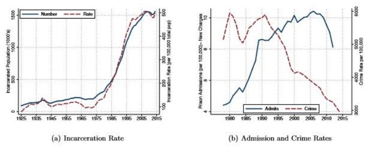
Figure 1. Crime rates from Uniform Crime Reporting Statistics (Federal Bureau of Investigation 2017). Incarceration rates 1925–1982 from Cahalan and Parsons (December 1986) and 1983–2016 from Carson and Mulako-Wangota (2017) include state and federal prisoners only. Admissions are from the National Prisoner Statistics Program for males in state and federal prisons admitted on new charges only (excludes parole/probation violations, etc.).
Literature
The literature on crime features few structural equilibrium approaches. Engelhardt, Rocheteau, and Rupert (2008) consider how the ability of employers to write efficient contracts tempers the labor market response to crime and vice versa. Huang, Laing, and Wang (2004) and Burdett, Lagos, and Wright (2003) study interactions with the labor market in search frameworks. The most related papers are İmrohoroğlu, Merlo, and Rupert (2004), Fella and Gallipoli (2014), and Engelhardt (2010). İmrohoroğlu, Merlo, and Rupert (2004) quantify the contributions of changes in apprehension probability, labor markets, and population aging to the decline in property crime.9Similar in spirit, Guner, Rauh, and Caucutt (2017) study the effect of the war on crime on the marriage gap between black and white men. Fella and Gallipoli (2014) also consider property crime but evaluate the impact of educational policy as well as punitive policy on crime. Engelhardt (2010) develops a model with rich heterogeneity to match the cross-sectional distribution of who commits property crime. Our work differs because we consider transitional dynamics and all types of crime. We have similar ingredients of many of these models: pecuniary considerations that differ based on life-cycle human capital growth and on employment status; and criminal capital or fixed heterogeneity to account for patterns of crime that pecuniary features alone cannot match within their respective frameworks. As will be come clear, we place extra care in parsing those components of heterogeneity that are decided early and those that depend on past criminal or labor market experience, as this is important for transition dynamics. The reader should also keep in mind that the fact that we target all types of crime causes our quantitative results to differ from the aforementioned papers as well as other structural approaches with similar ingredients that focus on property crime alone.10For example, see Fu and Wolpin (2018). Lochner (2004) considers property and violent crime but omits drug crime included in this analysis.
2. A Simple Model of Criminal Persistence with Empirical Cohort Evidence
In this section, we develop a simple model with two goals: (1) to illustrate the dynamic response to policy changes when criminality is persistent; and (2) to provide empirical evidence consistent with the assumptions and predictions of the theory.11There are other theories for each of the cohort effects and shifting age profiles that we document in the US data from 1980 to 2010. However, an appealing feature of the theory we present is that it parsimoniously predicts these two features of the data as well as the changing intensive and extensive margins of crime documented in US data over the same period, (see section 6). The model features three key ingredients. First, there is an age profile for crime. Second, the youth crime decision is decreasing in the probability of imprisonment and has a persistent impact on crime throughout life. Third, a prison experience can increase future criminality. Let  and
and  be the crime and incarceration rates, respectively, of cohort
  at time
  . Let the relationship between these variables over time be provided by the following equations.
Incarceration Rate 
Initial Crime Choice 
Evolution of Crime Rate 
The policy variable is  : the probability of incarceration, conditional on committing a crime. It is exogenous and can change over time. Assuming a large population, the incarceration rate for cohort at time is equal to that cohort’s crime rate multiplied by the incarceration probability .
The remaining equations explicate an extreme version of the cohort effects found in the full structural model. In the full model, choices made under previous policies persistently affect outcomes even as the policy changes later in life. Here, we model that cohort effect as a persistent component  , a function of both an initial crime choice and the policies uniquely experienced by a cohort over its life-cycle.12If the policy does not change over time, then there are no cohort or time effects. The initial choice is given by a function
 ![g^X(\pi) \in[0,1]](https://www.thecgo.org/wp-content/ql-cache/quicklatex.com-c1b4248893a2eddca21154af5e50a165_l3.svg "Rendered by QuickLaTeX.com") . We assume this function is twice continuously differentiable in (0,1) and that
. We assume this function is twice continuously differentiable in (0,1) and that  (i.e., that punitive policy deters).
The final two lines show the evolution of a cohort’s crime rate. An age profile is provided both by a policy-invariant rate of life-cycle growth or decay  and by the impact of past crime and incarceration through the coefficient term (Ø + βπ
 ).13This specification using age as a growth rate is key for econometric identification. It is conceptually motivated by the empirical profiles of crime as shown in detail in the online appendix and by the life course and turning point theories in sociology (Elder Jr. 1985). The coefficient term
  relating to
  has the following interpretation. The term
  captures the direct effect crime today has on crime tomorrow. The term
  captures the effect that a prison experience yesterday has on crime today. We assume
  , in which case a prison experience increases future crime or at least slows its decay.14Incarceration reforms can be studied for the case of
  , but as we show, it seems empirically unlikelyBoth
  and
and  can be interpreted as some persistent criminal capital, formed either by doing crime or by going through prison.15 The transitory level effect
  is unrelated to policy and will serve as a residual in the estimation.
The first set of predictions of this model, summarized in proposition 2.1 and corollary 2.2, explicate that cohort effects can generate a dynamic transition following an increase in  .15The proofs here consider transition dynamics and look at relative quantities of crime, either across generations or across ages for a single cohort. The online appendix presents additional propositions and proofs concerning comparative statics on aggregate crime and incarceration levels with respect to the policy . They show that crime and incarceration levels can either increase or decrease in response to an increase in , depending on parameters. While the cohort effects are always present, whether the transition is non-monotone requires the elasticity of the initial crime choice to be large relative to the change in
  . In other words, the impact of a prison experience on criminal persistence cannot be too large relative to the early life deterrence. A sufficient condition is if crime falls in the new steady state, but this is not necessary. Taken together, proposition 2.1 and corollary 2.2 illustrate the importance of dynamics for policy evaluation in two ways. First, it shows that the timing of evaluating outcomes matters. Crime decreases less in the short run than in the new steady state. Incarceration increases more in the short run than in the final steady state. Second, it shows that the costs and benefits of policy changes are borne differentially across cohorts.
Proposition 2.1 (The cohort born immediately before an increase in π has higher age-specific crime and incarceration rates at all ages than all cohorts it precedes and follows.). Let an initial π0 be given. Denote with hat notation the variables related to the cohort born at  where
where  is when the policy is changed to
  . Then:
![\[\begin{aligned} & C_{\hat{\jmath}, t}>C_{s, t-\hat{\jmath}+s} \quad \forall \quad t>\bar{t}+1 \quad \text { and } \quad s \neq \bar{t}+1 \\ & I_{\hat{\jmath}, t}>\quad I_{s, t-\hat{\jmath}+s} \quad \forall \quad t>\bar{t} \quad \text { and } \quad s \neq \bar{t} \\ & \end{aligned}\]](https://www.thecgo.org/wp-content/ql-cache/quicklatex.com-fdabce4abc46f65742ffb1bd7e9caafe_l3.svg "Rendered by QuickLaTeX.com")
See online appendix.
Empirical trends in age-specific arrest and imprisonment rates are suggestive of cohort effects. Figure 2(a) shows that the peak of the arrest rate for men age 25 to 29 occurred in the late 1980s, the peak for ages 35 to 39 in the late 1990s, and the peak for ages 45 to 49 in the late 2000s. In other words, the peak for each age group coincides with the same cohort born in the mid-1960s. Figure 2(b) conveys a similar story for prison admission rates on new charges (not parole or probation violations).
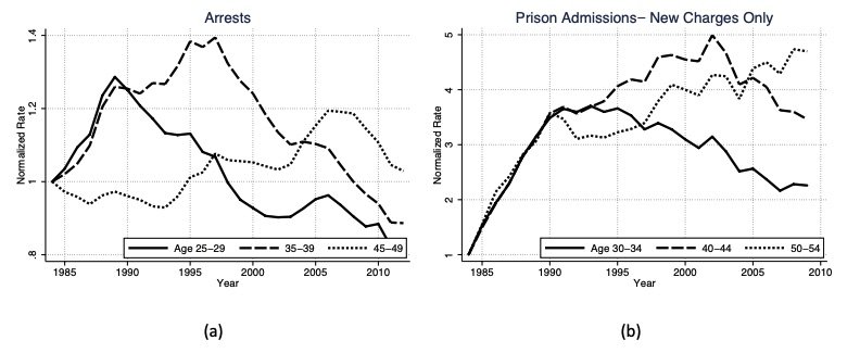
Figure 2. Cohort Evidence: Prison admissions from National Corrections Reporting Program Data and restricted to admissions on new charges only. Arrests from FBI crime reports accessed through the Bureau of Justice Statistics.
Corollary 2.2 (The transition paths of crime and incarceration after an increase in punitiveness are nonmonotone if the elasticity of the initial choice is sufficiently large relative to the effect of prison on criminal persistence.). Let an initial π0 be given and consider the economy at a steady state for that  . Assume at time-zero the policy switches permanently and unexpectedly to
  . Then:
a) The transition path for crime is non-monotone iff
![\[\frac{g^x\left(\pi_0\right)}{g^x\left(\pi_1\right)}>\frac{\sum_{a=0}^{M-1}\left(\phi+\beta \pi_1\right)^a+1}{\sum_{a=0}^{M-1}\left(\phi+\beta \pi_0\right)^a+1}\]](https://www.thecgo.org/wp-content/ql-cache/quicklatex.com-3e9838a87b6b391c0d138f99d970b62b_l3.svg "Rendered by QuickLaTeX.com")
b) The transition path for crime is non-monotone iff
![\[\frac{\pi_0 g^x\left(\pi_0\right)}{\pi_1 g^x\left(\pi_1\right)}>\frac{\sum_{a=0}^{M-1}\left(\phi+\beta \pi_1\right)^a+1}{\sum_{a=0}^{M-1}\left(\phi+\beta \pi_0\right)^a+1}\]](https://www.thecgo.org/wp-content/ql-cache/quicklatex.com-e813d316606a933bed7466ce3acadc26_l3.svg "Rendered by QuickLaTeX.com")
Proof. See online appendix.
The second result from this model is summarized in proposition 2.3. It states that if a prison experience increases criminal persistence, then the age profile of crime looks different in steady states with different incarceration probabilities π. In particular, as increases, crime is more persistent over the life-cycle, resulting in higher incarceration rates for old individuals relative to young.
Proposition 2.3 (If a prison experience increases criminality, then a steady state with a higher incarceration policy exhibits higher crime and incarceration at older ages relative to young.). Let two policies  be given and
  and
and  be the persistent component of crime at age
  in the steady state for each policy, respectively. Then:
![\[\frac{\hat{X}_a}{\hat{X}_{a-s}}>\frac{X_a}{X_{a-s}} \quad \forall \quad s \in(1, a)\]](https://www.thecgo.org/wp-content/ql-cache/quicklatex.com-47412f43eedd297b5e3d7286ea1113e6_l3.svg "Rendered by QuickLaTeX.com")
Proof. See online appendix. The change in the life-cycle profile at the steady state when the policy increases occurs when a prison experience slows the life-cycle decay of crime. While crime decays monotonically over the life-cycle, incarceration is hump-shaped. Applying this model to incarceration predicts that the peak of life-cycle crime will move to older ages for sufficiently large. This result is particularly important for how we think about time and age effects in the data. It is consistent with shifts towards deviance at older ages that are shown to be salient in the data, as seen in figure 3. It also suggests that only a portion of this shift is a permanent component, interpreted as the effect of changes in policy. Both the permanent shift and the transitory cohort effect from a simulation of the simple model can be seen in figure 4 as an additional visual check on our propositions.16We consider an arbitrary calibration for illustrative purposes. Parameter values are set to:  , and 8 age groups. The policy change considered a change in from
  to
to  .
.
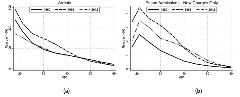
Figure 3. Permanent and Cohort Shifts in Age Profiles (Data): Prison admissions from National Corrections Reporting Program Data and restricted to admissions on new charges only. Arrests from FBI crime reports accessed through the Bureau of Justice Statistics.
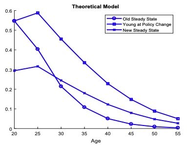
Figure 4. Permanent and Cohort Shifts in age profiles of crime rates as simulated from simple model
Figure 5 illustrates the point that the inclusion of both the persistence of prior choices made under old policies  and the assumption that incarceration increases (or slows the decay of) future deviance (
 are critical for providing cohort effects that generate a non-monotonic transition. The baseline features both ingredients. The line “No Early Choice” sets initial crime
  as a constant independent of policy . In this case, crime monotonically increases when policy increases at time 0. The line “No Prison Persistence” sets the impact of a prison experience on future crime to zero (
 ). In this case, crime monotonically decreases when policy increases at time 0. Incarceration is similar, except both the non-monotonicity and the final steady state levels depend on the elasticity of the crime choice with respect to the policy . A non-monotone transition and a smaller increase in incarceration (or even a decrease) in the final steady state are more likely when this elasticity is low. This is an important point for multiple reasons. It verifies that in order to replicate cohort features of the data, we need both an early life choice and for prison to affect future criminality. It also strikes at the policy crux of the paper. These two mechanisms make policy evaluation using observed outcomes difficult because results depend on the timing of the evaluation. These two mechanisms also imply the costs and benefits of a policy change differ across cohorts. 17Durlauf, Navarro, and Rivers (2010) summarize the range of assumptions required to employ aggregate regressions to estimate deterrence of policy within even a steady state framework.
Evidence of Cohort Effects
Cohort effects are a unique testable prediction of the theory.18See the online appendix for details of the dataset and variable construction. The appendix also presents results for three additional regression specifications: (i) a time-invariant age profile; (ii) linear regression with age omitted; and (iii) linear regression with time omitted. The results of the simple theoretical model refine the regression approach to separating age, time, and cohort effects in the data.19This is an important contribution to the criminal justice literature, which has mostly focused on the changing age-structure of prison admissions, something we demonstrate can be attributed partially to cohort effects. Consistent with empirical age profiles, we assume age affects the decay in crime over the life-cycle. However, one must take into consideration the prediction that crime should become more persistent over the life-cycle in response to a permanent increase in the probability of imprisonment for a crime π. 20This strategy relates to Schulhofer-Wohl and Yang (2016). We overcome co-linearity by placing more structure on the nature of the age effects. We also directly address the issue raised in Schulhofer-Wohl and Yang (2016), advocating that the age effect may be changing over time and cohorts. In using theory to identify where the age effect is negligible, an alternative approach would follow (Lagakos et al. 2016). Together these effects form the shape of the life-cycle profile, and the remainder time and cohort effects adjust the level. The full regression specification is:
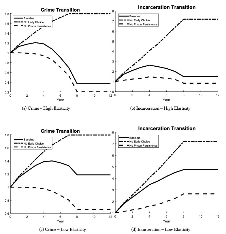
Figure 5. Crime and Incarceration over a Transition in the Simulation of the Simple Model. The first row sets the elasticity of the initial crime choice to be high with respect to the probability of prison condition on committing a crime. The second row sets the elasticity of the initial crime choice to be low with respect to the probability of prison condition on committing a crime.
![\[\begin{array}{r} I_{a, c, t}=\left(\beta^T \mathbf{D}^{\mathbf{T}}+\beta^C \mathbf{D}^{\mathbf{C}}\right) *\left(\beta^A \mathbf{D}^{\mathbf{A}} * \beta^Y \mathbf{D}^{\mathbf{T}}\right) \\ \text { st } \\ \beta^Y=0 \text { if } a<26 \\ \beta^Y \geq 1 \text { if } a>25 \end{array}\]](https://www.thecgo.org/wp-content/ql-cache/quicklatex.com-84eda50cc4f9e8f4589faaca75106ae6_l3.svg "Rendered by QuickLaTeX.com")
The dependent variable is prison admission rate for new charges only. The independent variables  ,
,  , and
, and  are respectively dummies for time, age, and cohorts.21The data for arrests only provides five-year age bands. Accordingly, we measure cohorts and time in five-year intervals. Although time enters in two ways, we refer to
  as the “time effect.” The cohort effect is
  . Age effects are multiplicative to time and cohort:
 . Finally, we allow the age effect to change over time (
 ) only after the peak of the life-cycle incarceration curve. We also impose that this coefficient be greater than or equal to 1 so that it only captures the flattening of the life-cycle profile.
We estimate the regression equation using non-linear least squares. The cohort and time coefficients are presented visually for incarceration and for arrests in figure 2. Looking at prison admissions, both time and cohort effects are significant. Time effects are around 50 percent larger in magnitude and are flatter across time varying only by about 25 percent from maximum to minimum. Cohort effects display a more dramatic non-monotonicity. They peak for the cohorts born in the mid 1960s, and both prior and future cohorts are around 60 percent lower. These facts together are consistent with our theory of how a more punitive incarceration policy should differentially affect cohorts. The 1960s cohort cultivated their criminal careers prior to the time-related increase in punitive admissions during the 1980s and were at the peak of their careers in their late twenties and early thirties (where behavior is less elastic) when the policy tightened.
We run the same estimation for arrests. The arrest data cover a larger number of states but are not limited to crimes that lead to a conviction, felony or otherwise. Still, although it is a noisy measure, it tells the same cohort story as the incarceration rates. A couple of interesting differences are that cohort effects are of a larger magnitude than time effects in arrest data and that the cohort effects in arrests appear to be trending upward again for cohorts born in the 1980s.
3. Quantitative Model
We present a quantitative model built on Burdett, Lagos, and Wright (2003) and Engelhardt, Rocheteau, and Rupert (2008) to show how punitive incarceration policy affects crime rates, incarceration rates, and labor market outcomes. Following Becker (1968), the main cost of crime is forgone labor market opportunities. Incarceration policy amplifies this cost through two channels. The first is at the individual level: an increase in the likelihood of incarceration increases the expectation of lost employment opportunities when an individual engages in crime. The second is at the aggregate level: incarceration policy and subsequent changes in the aggregate crime rate can decrease job arrival rates if firms’ profits suffer and they respond by creating fewer jobs.
Time is continuous. The economy is populated by a continuum of finitely lived, ex-ante identical individuals and identical firms. Individuals have linear preferences over consumption and discount the future at rate  . At any point in time, individuals can be in any of three labor market states: (i) employment; (ii) unemployment; or (iii) incarcerated. Employed individuals are currently matched with one firm. Unemployed individuals are those agents not currently matched with a firm but searching for a job. Lastly, incarcerated individuals are those agents currently in prison.
3.1 An Individual’s Problem
Unemployed individuals receive flow consumption b. Employment opportunities arrive at the Poisson rate  . All jobs are identical. Upon receiving a job opportunity, an unemployed individual can either accept the offer or reject it. If he accepts, he will become employed and receive a flow wage proportional to his human capital (productivity) level:
  , where
  is the wage level per human capital and
  is the current human capital level of the individual. Employed individuals receive job separation shock at Poisson rate
  , upon which they become unemployed.
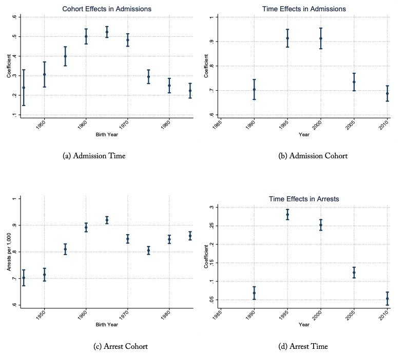
Figure 6. Estimated Cohort Effects: Prison admissions from National Corrections Reporting Program Data and restricted to admissions on new charges only. Arrests from FBI crime reports accessed through the Bureau of Justice Statistics.
All individuals outside of the prison receive crime opportunities at age-dependent Poisson rate  . Crime opportunities are characterized by an instantaneous reward of
  . These rewards are drawn from a common distribution
  . The reward associated with a particular crime opportunity is observed to the individual before they make the choice of whether to commit the crime or not. If he chose to commit the crime, he receives the reward and, with probability , he is caught and sent to prison.
Incarcerated individuals receive zero flow benefit while incarcerated. They receive a prison exit shock at rate  , upon which they are released and become unemployed.
We allow for several sources of heterogeneity across individuals: criminal capital, human capital, incarceration experience, and age. The latter two sources (incarceration experience and age) provide an important link from the model to the data. They allow us to study the heterogeneous effects of the criminal policies for individuals along observable dimensions. The first two sources (criminal and human capital) are important for the quantitative performance of the model along dimensions that are not accounted for by observables. They will also contribute to the persistence of criminality and help generate the cohort effects that we have found in section 2.
Labor market opportunities result in additional ex-post heterogeneity across individuals. Luck in job arrival and separation shocks, as well as incarceration incidence following a crime, generate different labor market statuses across individuals.
To better match the data along several dimensions, we introduce heterogeneity in criminal capital.22Nagin and Paternoster (2000) provide a review of the literature documenting “state dependence” in criminal activity based on past crimes, controlling for other factors. This is exactly what the assumption of criminal capital is meant to capture. We assume two types of criminal capital: low ( ) and high (
 ). Both types probabilistically receive crime opportunities drawn from the criminal reward distribution and decide whether or not they are worth committing. We call these crimes “rational crimes.” High criminal capital types uniquely receive additional crime opportunities at the rate
  that they must commit. These crimes bring no instantaneous benefit to the individual. We call these crimes “irrational crimes.” All individuals are born with low criminal capital. Upon committing a crime, a low criminal capital type becomes high criminal capital type at the Poisson rate
  . Criminal capital can also be built in prison.23Empirical evidence is provided by Bayer, Hjalmarsson, and Pozen (2009), using proximity to offenders by type in Florida prisons. During each period in prison, a low criminal capital type becomes high criminal capital type at the Poisson rate
  . A high criminal capital type becomes a low criminal capital type each period at age-dependent Poisson rate
  . 24This captures “turning points” associated with aging that deter crime and are not modeled explicitly following a literature harmonized by Laub and Sampson (1990, 1993). These turning points include things like marriage, children, and even physical deterioration. This feature is instrumental in the model to match recidivism rates in the data that otherwise could not be accounted for. Recidivism rates are important because, for a given amount of crime, they dictate the share of the population engaged in crime by pinning down individuals’ crime intensities. In section 6.2 we show that a model estimated without this ingredient is counterfactual to the data in a way that skews the policy implications of the model.
The third ex-post heterogeneity happens due to stochastic changes in human capital. Each individual is endowed with an initial human capital level, identical across individuals. We assume that human capital stochastically increases on the job and stochastically decreases while unemployed or incarcerated. We assume that human capital shock arrives at the Poisson rate  , and upon arrival human capital evolves according to labor status dependent function
  , given current human capital level . That is,
  where
where  is an indicator for the labor market state of the individual.
The fourth dimension of heterogeneity is a criminal record signifying past imprisonment observable by employers. As a result, there will be two types of jobs in the economy: one for individuals who have never been incarcerated, called non-flagged individuals, and one for individuals who have been incarcerated at least once, called flagged individuals. We denote  as the flag type;
  refers to non-flagged, and
  refers to a flagged individual. The main motivation for including this feature is to capture the fact that, in real life, criminal records are accessible by employers, and the size of the equilibrium effect of this access on both workers with records and those without is very much an open question.25Harmonized electronic records across jurisdictions began to be available in the mid-1990s. However, analyzing the impacts of record access is non-trivial because access remained highly variable across states for over a decade. Also, explicit records are unlikely to be the only avenue through which criminal history could be ascertained. These issues are beyond the scope of this paper. Although employers cannot observe certain characteristics of the individuals, (e.g., future crime propensities), employers can extract some information through individuals’ incarceration experiences summarized by this flag. So, in the model, this flag indicator will play the signalling role for the employers to infer the crime propensity of the individual.
The last dimension of heterogeneity is the age dimension. Age  individuals become age
  at the Poisson rate
  .26Stochastic aging is a standard method of reducing the state space (in this case to 3 age groups instead of 2,392 age-weeks) to make the computation feasible. They live at most to the age of
  . When age individuals receive aging shock, they exit the economy by receiving zero utility, and they are replaced with age 1 individuals who start life unemployed, with the lowest skill level and criminal capital.
3.2 Matching
We assume that employers can observe the flag type and the age of the individuals  . They create jobs conditional on these traits. This segments the economy into 2M labor markets because workers search only for jobs suitable to their observable traits. We assume that each type of the labor market is modeled as in Pissarides (1985). That is, unemployed workers and employers with vacant jobs meet randomly according to an aggregate matching function,
  , where
  is the number of unemployed workers with flag type and age , and
  is the number of vacant jobs for individuals with flag type and age . We assume that the matching function is strictly increasing in both terms and has constant returns to scale. The job arrival rate for workers is expressed as:
![\[\lambda_w^{k, m}=M\left(u_{k m}, v_{k m}\right) / u_{k m}=M\left(1, v_{k m} / u_{k m}\right)=M\left(1, \theta_{k m}\right)\]](https://www.thecgo.org/wp-content/ql-cache/quicklatex.com-2a9a8098d5642946f682fd9b0804c8b7_l3.svg "Rendered by QuickLaTeX.com")
where  is the market tightness for type
  jobs. Similarly, vacant job filling rate for firms is expressed as:
![\[\lambda_f^{k, m}=M\left(u_{k m}, v_{k m}\right) / v_{k m}=M\left(u_{k m} / v_{k m}, 1\right)=M\left(1 / \theta_{k m}, 1\right)=\lambda_w^{k, m} / \theta_{k m}\]](https://www.thecgo.org/wp-content/ql-cache/quicklatex.com-fe03079a702a76002443c1d5a328da84_l3.svg "Rendered by QuickLaTeX.com")
3.3 A Firm’s Problem
Now we turn to a firm’s problem: firms incur a flow cost to post a vacancy. Upon meeting with a worker, the match turns into an employment contract as long as the surplus of the match is positive. By hiring a worker with human capital , the match produces  , the worker receives a wage , and the firm collects profits
  . The match dissolves if either (i) the worker receives a separation shock; or (ii) the worker commits a crime and gets caught.
3.4 Early Life Choice
Finally, we allow for an early life choice that affects later criminal activity and is irreversible. We assume that at the beginning of life, individuals can pay a cost to increase their crime arrival rate  . Once it is chosen it will be fixed for the rest of individual’s life. The motivation behind such a choice is related to the near consensus reached across economics, sociology, and criminology that early life choices are instrumental in later life outcomes. For instance, young people’s lives can be forever impacted by the friends they choose or by the level of effort they exert in school. Their parents’ choices are also impactful. For our purposes, this feature will pick up the residual cohort effects documented in the data that cannot be accounted for by the criminal persistence provided by other features of the model. It accounts for the limited elasticity of criminal behavior for cohorts born prior to a policy change. Specifically, we assume that individuals choose their crime arrival rates by solving the following problem:
![\[\max _\eta-A \frac{\eta^\rho}{\rho}+E V_u^{1,0}\left(h_0 ; \eta\right)\]](https://www.thecgo.org/wp-content/ql-cache/quicklatex.com-1c1db1a5a57f70e4fc5239663dbb6eea_l3.svg "Rendered by QuickLaTeX.com")
where A and ρ are parameters to be calibrated. The first term in the above optimization problem,  , captures, in a reduced form, the unmodeled costs of choosing a higher crime arrival rate . 27These costs include forgone education opportunities and higher income opportunities associated with that and any nonpecuniary costs of being associated in higher crime activities. To be clear, there is no ex-ante heterogeneity across individuals in the model; in the stationary environment individuals will choose exactly the same crime arrival rate. However, when we study the transitional dynamics, that will generate heterogeneity in crime arrival rates across cohorts since along the transition the return to crime will be changing. In the online appendix, we provide several analytical predictions of a simpler model to illustrate the mechanisms discussed intuitively and decomposed quantitatively in section 6.
4. Calibration and Estimation
We calibrate our model such that the initial steady state replicates empirical moments from the late 1970s and early 1980s according to data availability. The assumption of a steady state at this time is motivated by the prior century of stable rates (see 1).29 While most parameters are jointly estimated to minimize the distance between the model and data statistics, we briefly provide a heuristic explanation of the moments most informative to different parameters. A full description of data sets, the calculation of target statistics, and the estimation procedure can be found in the online appendix.
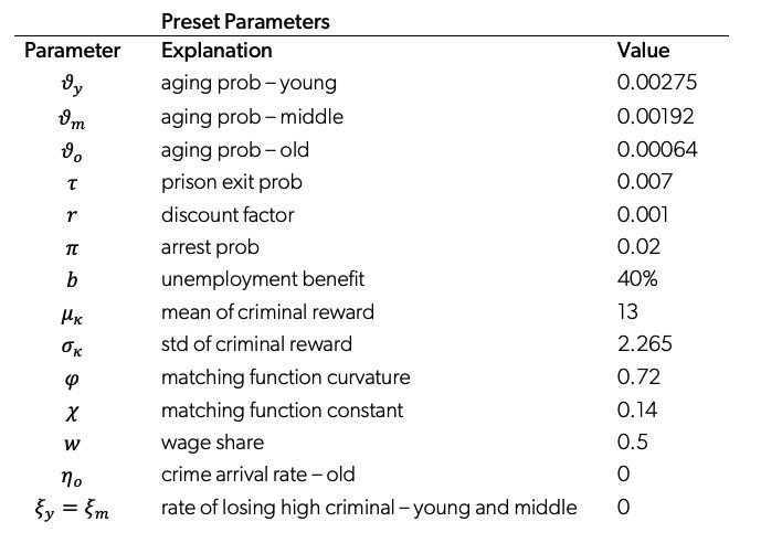
4.1 Externally Calibrated Parameters
The time period is set to be one week. We assume that on average, young individuals live for 7 years (between ages 18 and 24), middle-age individuals live for 10 years (between ages 25 and 34), and old individuals live for 30 years (between ages 35 and 64).28The average lifetime for each age group implies the stochastic aging probabilities of  for the young, middle, and old, respectively. We set the prison exit probability to 0.007 implying 2.7 years of prison time on average, consistent with Raphael and Stoll (2009).29Raphael and Stoll (2009) also show that increases in admissions rates on new charges account for more than half of the rise in incarceration rates and, when combined with parole failure, would account for 90 percent. This leaves little room for considering changes in length of incarceration spells, and so we do not include this. The probability of getting caught upon committing a crime, , is set to 2 percent, in accordance with our own calculations, which are consistent with Pettit (2012).30Please see the online appendix for details of our calculation of this number.
We choose  to provide an annual discount factor of 0.95. We assume that the criminal reward is drawn from a log-normal distribution with mean
  and standard deviation
  . We set
  and calibrate σk to equal one half of the average annual labor income.3133 This gives us
  .
.
We follow Shimer (2005) for the matching function:
![\[M(u, v)=\chi u^{\varphi} v^{1-\varphi}\]](https://www.thecgo.org/wp-content/ql-cache/quicklatex.com-1bc9ea614bcab0a3a4fa5b640adc4ccb_l3.svg "Rendered by QuickLaTeX.com")
where  is the unemployment rate and v is the vacancy rate. As in the Shimer (2005) study of U.S. aggregate data, we set the flow utility of unemployment
  to equal 40 percent, the matching function curvature
  to 0.72, and the matching function constant
  to 0.14. We assume that when workers and firms meet, they share the surplus equally, so we set the wage to be 50 percent of the productivity of the worker.
Table 1 shows the externally calibrated parameter values of the model.
4.2 Internally Calibrated Parameters
The rest of the parameters in the model are calibrated jointly by minimizing the percentage deviation of the model-generated moments from the data moments.
Labor Market Parameters
There are two parameters related to labor markets: exogenous job separation rate and vacancy cost. As in the literature, we calibrate these parameters to match average employment rates in the 1980s of black and white men between the ages of 18 and 34 without a high school diploma (71 percent, as calculated from the 1980 US census) and the median non-employment duration of this population (20 weeks, as calculated from the NLSY79).32Census data accessed through IPUMS, Ruggles et al. (2018). Data from National Longitudinal Survey of Youth (NLSY79) was accessed through the Bureau of Labor Statistics, US Department of Labor (2014) and is for the 1979 cohort only
Human Capital Parameters
We consider human capital to evolve on an exponential grid with an exponent  . 33We set the support of the human capital process as
  and
and  . Given this support, we space N grid points between and
  such that
  for every
  . We set
  in the estimation. This curvature replicates the concave human capital process prevalent in the data in a similar way as Kitao, Ljungqvist, and Sargent (2017). Although estimated parameters change, results are quantitatively and qualitatively robust to the number of grid points and the support. As in Ljungqvist and Sargent (1998), we assume a constant probability that human capital increases by one level during each period of employment, and we assume a different constant probability that it decreases by one level while either unemployed or incarcerated. We estimate the curvature ς jointly with the arrival rates of the human capital shock when employed,
  , and when non-employed (unemployed or incarcerated),
  , by the method of indirect inference. The goal is to replicate in model-generated data the coefficients from the following regression relating spells of employment and non-employment to wages estimated in the National Longitudinal Survey of Youth (NLSY79):
![\[\ln \left(w_{i t}\right)=\alpha+\beta^A A_{i t}+\beta^{A 2}\left(A_{i t}\right)^2+\beta^N N_{i t}+\beta^{N 2}\left(N_{i t}\right)^2+\gamma_i+\epsilon_{i t}\]](https://www.thecgo.org/wp-content/ql-cache/quicklatex.com-6d46d3c85cc7a1cc15734b34f4933175_l3.svg "Rendered by QuickLaTeX.com")
where  is the observed wages for employed individual
  at time ,
  is the age of the individual,
  is the months of non-employment in the last two years (including unemployment, non-participation, and incarceration), and
  is the individual fixed effects. We included the square terms for age and nonemployment spell to capture the non-linearities in the human capital process incorporated in the model data via the curvature parameter .
We create a panel identical to the NLSY79 using the simulated data from the model on which to run the same regression. It features the same number of individuals and the individuals’ actual ages in years. We transform the weekly model data to a monthly frequency as in the NLSY79, using the maximum wage of the individual in the last month as wage observation.
Crime Parameters
Crime opportunities are exogenous and arrive at the same rate when employed or unemployed. The calibration targets informative about these parameters are incarceration rates.34The median exit rate is observable and calibrated directly, leaving inflow rates to be inferred in order to match the share of persons incarcerated in the initial steady state.We assume the crime arrival rate for young and middle-age individuals with zero criminal capital are the same  . We set the crime arrival rate for the old individuals with zero criminal capital to 0
  . The underlying assumption of this empirical strategy is that all crime of the old is done by individuals who have committed crimes in their young or middle age years. This assumption is motivated by the very low admission rate of individuals over age 34 with clean criminal records (<1 percent, authors’ calculations from NACJD data).
Criminal capital is binary: high or low. There are four parameters related to criminal capital process: (1) the probability of gaining high criminal capital after committing a crime without being incarcerated, ; (2) the probability of gaining high criminal capital when incarcerated,  ; (3) the probability of losing high criminal capital,
  . We assume that only old individuals can lose high criminal capital. For young and middle-age individuals, we set
  . This allows us to identify
  by targeting the incarceration rate of old individuals.
Statistics on repeated incarceration are informative about the share of high criminal capital types and the additional crimes they commit. We add to our estimation targets the three-year re-imprisonment rate for the released prisoners.35These rates are calculated using the BJS Recidivism of Prisoners Released Series published by the United States Department of Justice (2011). In order to be consistent with the concept of incarceration and crime used in the model and in targets from other datasets, we take care to only include those who are re-imprisoned on a new felony conviction. This excludes those reincarcerated in jails or re-imprisoned for violations of conditions of their parole, probation, or other conditions of release. The details of these data and our calculations can be found in the online appendix. This rate is 20 percent among young and middle age groups in the data.
The next target is the fraction of the population who are incarcerated by the age of 35. In the data, 19 percent of individuals have been to jail or prison at least one time by the age of 35 (NLSY79). In the model, the probability of gaining criminal capital, v, is a crucial parameter to capture this fact. If  , crime will be more widespread among the population, whereas as becomes larger, crime will be concentrated among a few individuals. The incarceration rate of old individuals (ages 35 to 64) disciplines the probability of losing the high criminal capital,
  . This is because we assume that only high criminal capital types receive crime opportunities when old. Using the National Archive of Criminal Justice Data (NACJD) and US census data, we calculate approximately 0.5 percent of the old population is incarcerated.
Finally, we include the change in the young-to-old incarceration ratio over 30 years as a target for our estimation. This ratio dropped by 40 percent in the NACJD data. We include this target because it is a key prediction of the simple model in section 2 supporting the mechanism that an incarceration experience increases future criminality (proposition 2.3). In the full model, the impact of an incarceration experience operates partially through the acquisition of criminal capital. In accordance with this calibration strategy, the shape of crime propensity over the life-cycle is also largely determined by the fraction of crimes committed by high criminal capital individuals versus low criminal capital individuals. If all the crimes are committed by high criminal capital individuals, deterrence is zero and the life-cycle profile is unaffected by changes in the policy.
Early Life Parameters
There are two parameters regarding the early life choice: those that determine the costs of choosing a higher crime arrival rate, and  in equation 3.3. Given the curvature parameter , we pick such that at the initial steady state, individuals choose the crime arrival rate pinned down by the estimation targeting the initial steady state. The parameter captures the elasticity of early life choice. If this choice is very elastic, the model generates a highly non-monotonic path for incarceration rate along the transition, whereas if the early life choice is inelastic, incarceration rate follows a more monotonic path. We calibrate this parameter to match the non-monotonicity of the time series of the incarceration rate of young individuals over the 30 years for which we have data. Since our model cannot capture the total change in incarceration, we target the ratio of the difference in the incarceration rate between 2009 and 1980 and the difference between the maximum incarceration rate within this period and the 1980 incarceration rate for young individuals. This ratio is 20 percent in the data.
Table 2. Calibrated Parameters
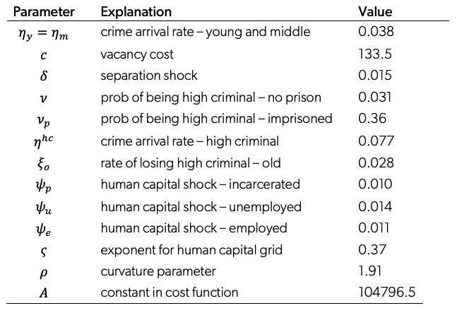
Data Note: Table 2 shows the internally calibrated parameters of the model. See the main text for a discussion of the explanation of these parameters and how they are identified in the model.
Table 2 shows the estimated parameters. Table 3 shows the performance of the model in matching the moments targeted. The model does a satisfactory job in capturing the moments targeted in the calibration.36In the online appendix, we discuss how removing elements such as criminal capital or prison flag compromises the model’s fit. We also provide robustness checks on some of the externally set parameters. Two remarks are in order. First, the estimated parameter for the early life choice, A, implies agents spend around 1.3 times the annual income in the model to increase criminal opportunities in the baseline. This may seem to be high, but this parameter captures all foregone opportunities of choosing a higher criminal path that are not modeled here. And second, the vacancy cost is also higher than other papers in the literature. The main reason for this is to match very low employment rate (71 percent) of our sample of interest: young and middle-age individuals with a high school education or less.
Table 3. Model Match
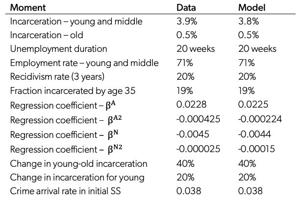
Data Note: Table 3 shows a comparison of empirical and simulated moments. See appendix for a detailed discussion for data sources on the empirical moments.
Table 4. Characteristics of Criminals
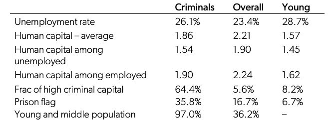
Data Note: Table 4 shows a comparison of various statistics for the individuals who commit crime and the overall population.
5. Steady-State Analysis
To better understand how a change in punitive policy affects crime, labor markets, and inequality, we first discuss the determinants of crime in the initial (pre-1980s) steady state.
Table 4 shows that criminals differ from the overall population along several dimensions. As expected, criminals are more likely to be younger and unemployed, with lower human capital and higher criminal capital, and more likely to have criminal records in their history. In the initial steady state, 74 percent of criminals are employed, compared to 77 percent of the general population. However, they are employed at a much lower wage. The human capital of criminals is on average around 20 percent lower than the population average (2.21 vs. 1.86). Given their respective distributions, the probability of weekly crime conditional on employment is 0.67 percent for the unemployed and 0.58 percent for the employed.
The most important dimension of these data is that the majority of the crimes are committed by individuals with high criminal capital and by previously incarcerated individuals. The fraction of all individuals with high criminal capital among the population is 5.6 percent, compared to 64.4 percent of the individuals who commit crime. Similarly, 16.7 percent of all individuals have a prison flag, compared to 35.8 percent of the individuals who commit crime. This implies that most crime is committed by “career criminals” and that criminal capital drives the recidivism prevalent in the data. Criminal careers are mostly ended by the loss of criminal capital in old age. Subsequently, individuals over 35 have a crime rate one-eighth of those younger than 35.
The next logical step is to ask what determines who begins crime in the first place. All individuals in the model draw from the same crime-reward distribution and face the same prison risk if they commit the crime. What may differ across individuals is what they lose by going to prison. These opportunity costs are increasing in human capital and higher for those currently employed. Figure 7 shows the probability of committing crime conditional on receiving an opportunity for young individuals without criminal capital or a prison flag. This probability decreases as human capital increases, notably at a faster rate for the lower half of the human capital range.
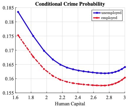
Figure 7. Determinants of Crime – Labor Status: Figure 7 shows model-generated crime probability conditional on receiving an opportunity as a function of human capital for a young individual with low criminal capital and a prison flag.
Whereas policy functions show the contribution of the current state to an individual’s crime entry choice, the impact on total crime in the economy depends on the distribution of individuals over this state. To better get at this contribution, we run a simple linear regression on individuals’ probabilities of committing crime within the week.37Specifically, the dependent variable uses the individual crime reward threshold to calculate the probability of receiving a crime reward above that threshold. Unemployed wage is the shadow wage. Table 5 presents the marginal effects of this regression. The average weekly crime probability in the economy is 0.77 percent per week, with a standard deviation of 1.8 percentage points and a maximum of 8.7 percent. Focusing on the middle column, we see the crime entry choice is responsive to labor market outcomes, but not overly so. An increase in one standard deviation of wages reduces crime by 4.5 percent to 5 percent, and gaining employment reduces crime by another 4.5 percent. These effects may seem small, but they reflect the data the model is calibrated to match. The variance in wages for this particular population of young men (those without any college-level education) is very small, so of course it does not provide much variation in crime outcomes. Furthermore, the separation rate from employment in the data is almost as high as the probability of going to prison if one commits a crime. This makes the opportunity cost of employment low. Criminal behavior in the data reflects this logic. We see most criminals are employed.38Criminals in the data do report lower wages, but we cannot see their wages at their first crime.
Table 5. Marginal Effects on Weekly Crime Probability
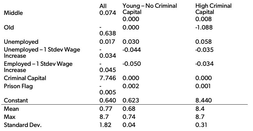
Data Note: Dependent variable is in basis points. For example, the mean weekly crime probability is 0.77 percent. The effects of a 1 standard deviation increase in wages considers the unconditional wage distribution for the column population.
If the crime entry decision is driven by luck, is there any hope that improving labor market opportunities can end a criminal career? According to figure 8(a), this is unlikely if an individual has accumulated high criminal capital. It shows that such individuals commit about 50 percent more crimes than those without criminal capital, regardless of their human capital. However, figure 8(b) is more optimistic. It shows that a prison record itself does not put an individual on this path of higher crime.
To summarize, the determinant of who commits crime is largely luck. Young individuals are similarly likely to enter a criminal path; it just depends on who draws a sufficient crime opportunity. From here criminal persistence is driven mostly by past criminal behavior through additional crimes among those with high criminal capital until this channel is eliminated by old age. This should not be interpreted as implying that economic conditions don’t matter. That is not true. For example, crimes arrive with 3.8 percent chance at a weekly frequency, but from this the young only take about the top 20 percent, so they are being picky. It is just that the impact of wages is diminished because wages are compressed for the population of low-skilled men we study, implying little variation in wages to affect variation in the likelihood of starting crime. However, if wages were raised for everybody, crime would go down (see section 6.7). This population also faces relatively high separation rates. This lowers the deterrence of having a job today since one may expect to lose that job by tomorrow.
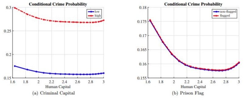
Figure 8. Determinants of Crime – Criminal Capital and Incarceration: Figures 8a and 8b both show model-generated crime probability conditional on receiving an opportunity as a function of human capital for a young employed individual. The left panel plots it across different criminal capital, and the right panel plots it for different incarceration experience. Flagged are the ones who have been to prison and unflagged are the ones who have never been to prison. The qualitative properties of the figures remain the same for the unemployed and middle-age individuals.
6. Punitive Incarceration Reform
In this section we study the effects of an increase in the probability of incarceration after committing a crime on aggregates like crime rates, incarceration rates, labor market variables, and inequality. We assume the probability of imprisonment for a crime () permanently and unexpectedly increases from the 1980s steady state of 2 percent to a higher value of 8 percent, similar to what we calculate for the United States in 2000.39See the online appendix for the assumptions we make in this calculation.
6.1 Steady-State Comparison
We begin by comparing steady states. To see how a change in affects the incarceration rate, consider the probability of incarceration for an individual with current state  :
:  . The overall crime rate is
  , where
  is the distribution of individuals across states. Increasing the probability of getting caught conditional on crime, affects the overall crime rate through three channels. The first is a direct “arithmetic” effect by increasing , holding all else constant. The second is an indirect deterrence effect through endogenous responses of the individuals of a given state . They increase their crime reward thresholds,
  , and decrease their early life criminal intensity choice, . The final effect is an indirect compositional effect through a change in the distribution of individuals across states . The endogenous job creation response of firms contributes to this effect.40The online appendix provides an analytic exposition of these effects within a simple model.
The deterrence channel lowers crime and mitigates the mechanical impact of the first arithmetic channel working to increase incarceration. Therefore, it is unclear whether an increase in will increase or decrease incarceration rates. If the deterrence effects are small, then the arithmetic effect of higher conditional probabilities can dominate and increase the overall incarceration rate. This typically generates a “Laffer curve” type of non-monotonicity between and the incarceration rate. In our model, it is also unclear that crime rates should fall. It is true that at every state s, individuals raise their threshold and commit less crime. However, in our model, a prison experience worsens an individual’s state and makes the individual more likely to do crime. In this way it is possible that an increase in π leading to an increase in incarceration will change the distribution of individuals across states enough to actually increase crime.41In section 12 of the online appendix, we plot the incarceration rate as a function of across steady states in the calibrated model. It is non-monotone.
Table 6 shows the comparison of steady states across two different criminal justice policy regimes. We find that, at the steady state, the direct arithmetic effect of the increase in dominates the other two channels. Incarceration increases as the criminal system becomes more punitive. We also find that deterrence (and incapacitation) overwhelm the third channel provided by the prison experience. Crime decreases as the criminal system becomes more punitive.42The strengths of these different channels depend on the magnitude of . In the appendix, we provide comparative statics on steady states with respect to illustrating this and the “Laffer Curve” effect.
Table 6. Steady-State Comparison
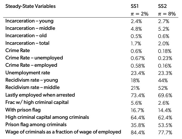
Data Note: Table 6 shows a comparison of two steady states, one with  and one with
  .
.
6.2 Transitional Dynamics
In section 2 we argued that when criminal behavior is persistent, the transition following a change in punitive policy can take several decades. This makes evaluation of the impact of the policy change difficult. It also makes policy design difficult because it provides unique costs associated with the policy change that are differentiated across cohorts. We then established the empirical relevance of this mechanism by showing cohort effects in the data. We now study quantitatively how the channels of criminal persistence included in our model affect these issues pertaining to the transition.
The left panel of figure 9(a) shows the evolution of the total incarceration rate along the transition. It starts at 1.7 percent, doubles in five years, and then gradually declines to the new steady-state level of 2 percent. Interpreting these figures through the lens of the simple theory in section 2, we see that the model calibrated to the 1980s steady state delivers a level of criminal persistence for those with criminal histories that is sufficiently inelastic and an early life choice to enter a criminal career that is sufficiently elastic to provide a non-monotone incarceration path over the transition. The criminal persistence of early cohorts engaged in crime under the old policy limits their response and drives the increase in incarceration rates in the short run. The response of the cohorts born under the new policy captures the full deterrent effect and drives the fall to the new steady state incarceration rate in the long run. The right panel of figure 9(a) further refines our understanding of these elasticities. The criminal persistence of those with criminal histories is not so large as to increase crime in the short run. The potential impact of the prison experience to increase criminality is also not so large as to increase crime at any point along the transition.
This non-monotone transition implied by the model calibrated to a steady state provides further evidence that the evaluation of punitive policy inferred from short-run effects is likely to be problematic for the US data. Measuring the increase in incarceration in the short and even medium run after the policy change provides little information about the eventual steady state effect unless interpreted through the lens of an overlapping generations model, such as the one we provide. It also shows that inferring the causal impact of changes in incarceration on crime using correlations between these time series is a deeply flawed approach. Crime falls as incarceration rises over the first 10 years of the transition, but crime also falls as incarceration falls as the transition continues to the new steady state. The correct comparison would be to compare steady states and observe that incarceration rises and crime falls as the policy becomes more punitive.
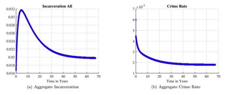
Figure 9. Incarceration and Crime Rate over the Transition: Aggregate crime rate is computed as the ratio of total crimes to the measure of non-incarcerated individuals.
The transition in the model is also consistent with the cohort empirical motivation of section 2 backing this theory. Figure 6.2 shows the evolution of incarceration rate is different for different age groups. The incarceration rate of young individuals reaches its maximum in around 3 years and converges to the steady-state level in around 30 years. However, the incarceration rate of old individuals reaches its maximum in around 10 years and converges to the new steady state in more than 50 years. In terms of magnitudes, the middle-aged group sees the largest rise in incarceration rates in the short term, but the old-aged individuals have the largest permanent rise in the new steady state.
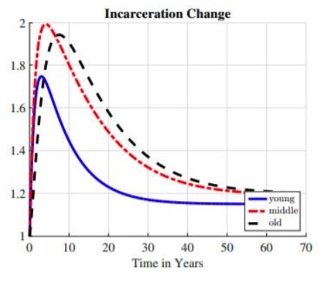
Figure 10. Incarceration Change by Age: The transition for different age groups relative to their initial steady-state levels.
The model does not generate a quadrupling of the incarceration rate as observed in the data, and it predicts a transition that is too quick compared to the data. However, this is not a failure because this was not our goal. Instead, this experiment is an accounting exercise to isolate the impact of changes in punitive policy alone. In reality, the policy was likely a reaction to changes in crime driven by other exogenous factors. In section 6.7 we explore whether changes in the benefit (crime reward) or opportunity cost (wages) can improve the model fit. With respect to the speed of the transition, we assume that the policy change is a sudden and one-time event. However, in practice, the de facto implementation of policy changes was more gradual than the de jure reforms.43A key constraint to such a drastic change in the use of punitive incarceration was capacity constraints. From 1985 through 1990, 50 to 70 percent of prisons were over capacity. In fiscal year 1990, Congress allocated an additional $1 billion for physical investment in expanding buildings and facilities. Since 1993, incidence of overcrowding has remained below 40 percent, according to James (2013).
It is still useful to understand that there is a maximum increase in incarceration we can generate by increasing π alone as agents respond by lowering their crime rates (as explained in our “Laffer curve” discussion). This holds for a similar reason even if we change the calibration to increase the role of criminal capital and irrational crime. As we increase the probability of gaining criminal capital or frequency of irrational crimes for those with high criminal capital, agents react by reducing the number of first crimes committed. This endogenous reaction limits the scope of criminal capital to increase the incarceration rate. In other words, the irrational crimes are not a free parameter that enable us to match whatever we want.
6.3 What Drives the Non-Monotonicity of Incarceration?
The extent of the rise in incarceration after a policy change and whether it rises more in the short run than in the long run depends on several factors. The full long-run deterrent effect is provided by changes in the early life choice, changes in the crime threshold rules of agents given a particular state, and changes over time in the distribution of agents over states. Figures 11(a) and 11(b) provide results of a counterfactual experiment in which we imagine if one or more of these factors were missing. The “benchmark” is the full model. The “no initial response” line keeps the early life choice fixed at the first steady state. The “no initial and firm response” line keeps both the early life choice and the market tightness fixed. The “no response” line keeps all endogenous decision rules fixed at the first steady state: the early life choice, the market tightness, and the crime thresholds of agents conditional on their state. In this final line, all that remains is that the change in policy moves people around to different states by sending them through prison more often.
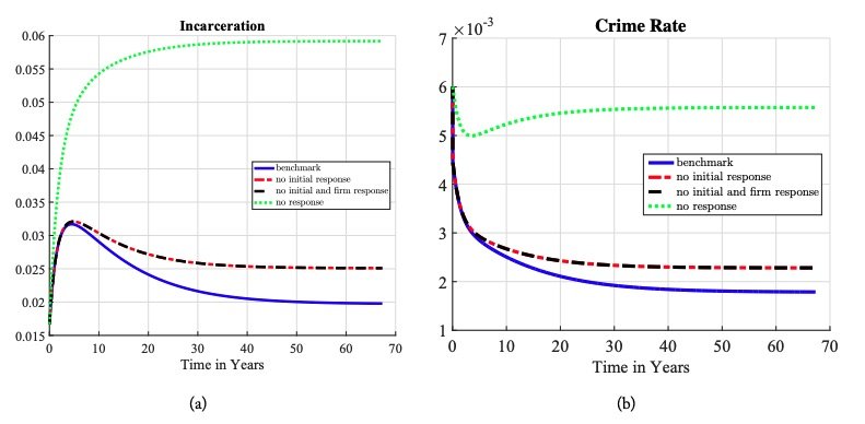
Figure 11. Incarceration and Crime Over Time: The solid line is the benchmark economy. The long dashed line is the economy when individuals keep their early life crime choices as in the first steady state. The dashed line is the economy when firms keep the same job creation level and individuals keep their initial choices as in the first steady state. Lastly, the dotted line is the economy when firms keep the same job creation level and individuals keep their initial and ex-post crime choices as in the first steady state.
The change in individuals’ crime thresholds at a given state is quantitatively the most important factor in the model. It provides the movement from the “no response” line to the “no initial and firm response” line. All along the human capital distribution, a typical agent raises his threshold enough to lower his crime probability by about 60 percent (See figure 12). This change in behavior reduces the rise in incarceration by about 81 percent at the new steady state relative to if there were no endogenous responses in the model by amplifying the fall in crime by nine-fold. This is the classic deterrence channel studied in the literature. These graphs also show that the role of this channel grows as time passes—it reduces the rise in the incarceration by only 36 percent at year 5 by only amplifying the fall in crime by three-fold. Again, to emphasize the point: the classic channel of deterrence on the decline in crime has previously studied comparing steady states only, and we find its importance increases three-fold from year 5 to year 30 along a transition.
The elasticity of the response of the early life choice of new generations to the observed policy change was estimated in our calibration strategy as a residual. We chose this parameter such that the model replicated the non-monotone shape of the prison admissions time series in the data. The estimated value implies a drop of crime arrival rates by about 25 percent, from 2.8 percent to 3.8 percent. Figures 11(a) and 11(b) show that this plays a modest but non-trivial deterrence role in the quantitative prediction: it moves from the “no initial response” line to the “benchmark” line. It plays a larger role in driving the nonmonotonicity, but still the classic deterrence channel of changing policy rules provides about half of the decline from the peak in the benchmark model. How does this work? Recall that luck is a major determinant of who commits crime—about two-thirds of crime is done by those who get good draws from the crime reward distribution as youths and who build criminal capital. The fall in the crime arrival rate due to the change in the early life choice lowers crime and incarceration by helping to lower the share of individuals engaged in crime in the population.
The change in the market tightness provided by changes in firms’ job posting behavior has near zero impact on incarceration and crime. This is not to say that the tightnesses of labor markets do not change. They do, as we discuss next in section 6.5. It is that the differential impact of employment and unemployment on decision rules governing the crime choice is very small. Therefore, changes in employment rates do not affect criminal behavior much.
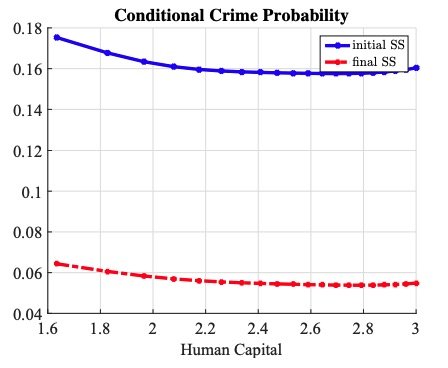
Figure 12. Crime Probability: Figure 12 shows the crime probability for an unemployed young individual as a function of human capital across two steady states.
6.4 The Contribution of Incapacitation versus Deterrence
The above discussion can also be reframed through the classic lens used by criminologists to study the impact of criminal justice reform, namely, incapacitation and deterrence effects. The incapacitation channel lowers crime by putting likely criminals in prison. The deterrence effect considers that more punitive policies lower crime by deterring individuals from committing crime in the first place. These effects are hard to measure in the data but easy to isolate in our structural model. The incapacitation effect is isolated in a counterfactual transition experiment by setting the time spent in prison to zero while maintaining the expected cumulative effects of prison on human capital, the prison flag, and criminal capital from the baseline model. The deterrence effect is isolated in a second counterfactual transition experiment by fixing the decision rules of the individuals and firms at the initial steady-state level along the transition.
Figure 13(b) shows that both incapacitation and deterrence work to lower the crime rate, but at different times and in different magnitudes. In the short run, the incapacitation effect dominates. This “cleansing” of the population is important in the short run because deterrence is limited by the inelasticity of individuals’ crime choice due to the channels of criminal persistence in our model. In the long run, when the full deterrent effect is realized, it dominates the incapacitation effect, each respectively accounting for about 80 percent and 20 percent of the total decline in crime at the new steady state.
Figures 13(c) and 13(d) show that both deterrence and incapacitation have significant effects on the employment and unemployment rates. The contribution of each channel is a bit by construction. While it is true that market tightness changes due to the response of firms’ vacancy posting, the dominant mechanism is the assumption that once an individual is released from prison, that individual is unemployed. Since we maintain the cumulative impact of prison in this experiment, removing either incapacitation or deterrence increases the likelihood that workers who commit crime will lose their jobs through this mechanism. It also provides the asymmetric effect of incapacitation and deterrence on employment. Without deterrence, employment permanently decreases by about 3 percent, due to the higher share of the population imprisoned. Without incapacitation, employment permanently increases by about 1 percent, due to a lower share of the population imprisoned, freeing more persons to be eligible to work. The asymmetry in these magnitudes highlights the firms’ responses and the increased number of released prisoners churning through unemployment.
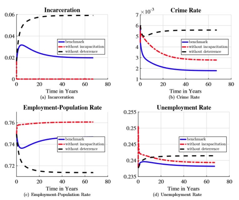
Figure 13. Incapacitation versus Deterrence: Incarceration, crime rate, employment-population ratio and unemployment rates along the transition without incapacitation or deterrence effects. The solid line is the benchmark economy. The long dashed line is the economy when incapacitation is eliminated. The dashed line is the economy when all decision rules of the individuals and firms stayed at the initial steady state levels
6.5 Labor Markets and Inequality
Our structural model provides a unique environment to study the impact of large changes in punitive policy on aggregate employment and wages. The response of aggregate employment is modest: employment falls 1.5 percentage points in the short run and recovers in almost 30 years. The impacts on younger agents and those with criminal records are larger. Figure 14(a) shows that middle-aged individuals experience the largest drop in employment—a decline of 4 percent. This is because this group experiences the largest increase in the incarceration rate (figure 6.2). Figure 14(b) shows individuals flagged with a criminal record experience a drop of around 6 percentage points in the employment-population ratio at the peak of the transition to 62 percent, compared to 76 percent for the general population.44Flagged types start with substantially lower employment population ratio with respect to non-flagged ones (68 percent vs. 76 percent).
The fact that these cross-sectional differences across age are only present in the transition shows how the policy generates inequity in employment opportunities for a cohort. This contrasts the permanent inequity provided for those with a criminal record as seen in figure 14(b). This is due to two reasons. First, the direct effect of increasing the probability of imprisonment conditional on committing a crime. As criminals churn more often through the prison, they are released to unemployment. The second reason is the endogenous response of firms’ vacancy posting behavior across labor markets, indexed by age and prison record flag, shown in figure 15(a). Recall that firms use observable information on an individual’s age and prison record flag to form expectations about the value of the match, conditional on the individual’s unobservable human capital and criminal capital. Market tightness falls permanently for those with a prison record flag, thus increasing unemployment duration because the information provided by a prison record flag changes. Crime becomes more concentrated within a small population after the policy change. This implies a prison flag is more indicative of high criminal capital; crime is mostly done by career criminals. Second, criminals cycle through prison more often and lose additional human capital after the policy change. This implies a prison flag is more indicative of low human capital.
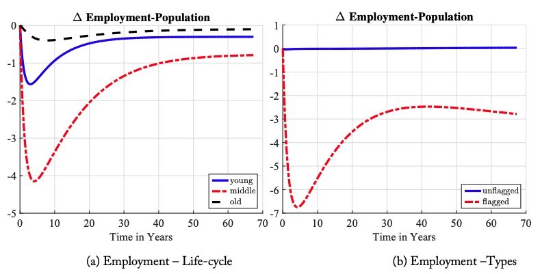
Figure 14. Employment across Different Groups: The left figure is across age dimensions, and the right figure compares the employment-population ratio for non-flagged individuals. Both are changes in percentage points relative to the initial steadystate level.
The dynamics of market tightness for the old clearly show the differential impacts of incapacitation, deterrence, and the prison experience over the transition. First, incapacitation dominates—the labor market is cleansed. Second, the prison effect kicks in—imprisoned workers are released with low human capital. Finally, full deterrence is realized—new cohorts chose lower crime arrival opportunities, thus increasing the expected duration of the match.
The magnitude of the difference in market tightness between those with and those without criminal records may seem smaller than expected. Our results should not be interpreted as saying that criminal records don’t matter. Instead, they say that criminal records don’t matter much through the mechanisms featured in the model, where the cost of hiring workers with criminal records is that they are likely to have low productivity and quit early. Alternative mechanisms could amplify these effects. For example, we make the assumption that wages are proportional to productivity. In reality, minimum wages likely truncate the distribution of wages above that of productivity, or efficiency wages could be operational. There may also be other costs inflicted on an employer after hiring an ex-convict. For example, the criminal may steal from an employer’s firm.
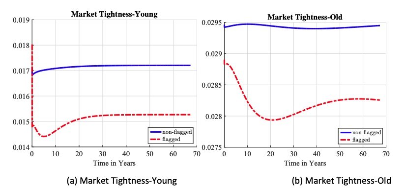
Figure 15. Market Tightness over Time: Figure 15(a) shows the dynamics of market tightness for the young individuals, both flagged and non-flagged. Figure 15(b) shows the same statistics for the old individuals.
The increased churning through prison also has a sizeable impact on wage inequality through the human capital depreciation channel. Figure 16(a) shows that this creates temporary wage inequality across cohorts, and figure 16(b) shows that this creates a large and permanent increase in wage inequality for those with a prison record. At the peak of the transition, human capital of those with a prison flag drops almost 8 percent and only recovers to a 7 percent decline when comparing the new steady state to the old. These figures show that the policy widens the economic gap between criminals and non-criminals substantially
Figures 17(a) and 17(b) illustrate the magnitudes of the mechanisms we have discussed using the same counterfactual decomposition we explained in section 6.2.
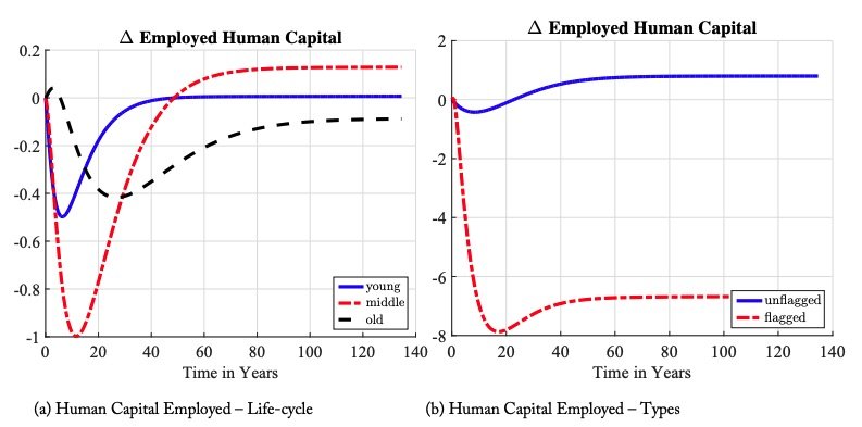
Figure 16. Human Capital across Different Groups: The figure on the left is across age dimension. The figure on the right is across the criminal record dimension. Both figures show percentage change from the initial steady-state level.
6.6 Role of the Model’s Assumptions
We now explore how our assumptions of the early life choice and criminal capital—relatively novel features of our theory—quantitatively contribute to these predictions of the model. Do we really need these? If so, why? To answer those questions, we consider how our results would look if we omitted each of the aforementioned features individually, re-estimated the model to best fit US data, and re-ran our transitional experiment.45More specifically, without prison flag, we re-estimate the model to target the same set of moments in the benchmark economy. The only difference is that without prison flag, we set the probability of being flagged after incarceration experience to 0. Without criminal capital, we are left with seven parameters to be calibrated: crime arrival rate, vacancy cost, job separation rate, human capital shock arrival rate for employed and unemployed, the human capital grid parameter, and the curvature of early life choice. As in the benchmark economy, we target incarceration rate for young and middle-age, employment-rate for young and middle-age, average unemployment duration in the whole population, the regression coefficients in equation 4.1 and the change in incarceration for young individuals over transition. The values of the parameters for each estimation is listed in the appendix. Figures 18(a) and 18(b) show the results. The prison flag has almost no impact on these aggregates, but this is something we learn from the model. We know that criminal records exist and are used in the labor market, but we learn that they have little impact on criminal behavior, at least through the channels we have in the model. Criminal capital is something not observed in the data and does change the results, so we focus the following discussion on why we have it.
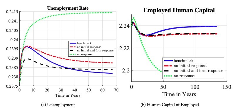
Figure 17. Labor Markets over Time: The figures show the decomposition of the evolution of the unemployment rate and human capital of employed individuals. The unemployment rate is the ratio of the unemployed to the labor force. The solid line is the benchmark economy. The long dashed line is the economy when individuals keep their early life crime choices as in the first steady state. The dashed line is the economy when firms keep the same job creation level and individuals keep their initial choices as in the first steady state. Lastly, the dotted line is the economy when firms keep the same job creation level and individuals keep their initial and ex-post crime choices as in the first steady state.
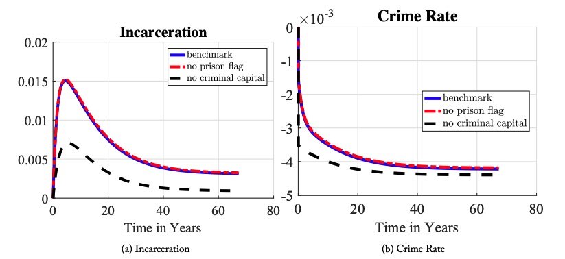
Figure 18. Model Assumptions: Figures 18(a) and 18(b) compare the evolution of the economy in response to the policy change for different model assumptions. The solid line plots the benchmark economy, the long dashed line plots model without prison flag, and the dashed line plots the model without criminal capital. In each case, parameters are re-calibrated to match certain moments of the data. See the text for a discussion of the re-calibration.
Criminal capital was added to the model to match a salient feature of criminal behavior: recidivism. The recidivism rate for released prisoners targeted in the calibration was 20 percent over three years after release in the early 1980s. When we re-estimate the model by dropping the criminal capital assumption, we can still generate a rise in incarceration, though at a much smaller magnitude. However, we can no longer match the initial steady state recidivism rate observed in the data. We undershoot by 6 percent. Furthermore, recidivism does not rise along the transition. This is also contrary to the data. Using the Recidivism among Released Prisoners report (United States Department of Justice 2011), we calculate that the average recidivism rate on new charges doubled from 17.8 percent in 1983 to 35 percent in a Florida sample from 2003 (Bhati 2010).46The recidivism rate increased to 27 percent in the 1994 iteration of the Recidivism Among Released Prisoners Series with the same design as the 1983 iteration. There is a version of these data for 2005, but we did not have access to the microdata and weren’t able to calculate the recidivism rate on new charges, as would be consistent with our quantitative analysis. See the online appendix for discussion of these datasets. See section 12 of the online appendix for graphs of recidivism dynamics disaggregated by age in both the model and data. Both show an increase and flattening of the age profile of recidivism.
The key difference between the calibration with and without criminal capital is who commits crimes. With criminal capital, crimes are concentrated among a few individuals with a very high crime rate. Without it, crime is spread across the population at lower rates for each individual. To achieve this, the calibration without criminal capital requires a much higher crime arrival rate. Interestingly, this increases the elasticity of crime to the policy change. When a larger distribution of people are committing crimes and the policy becomes tougher, the fall in crime is larger. This limits the model’s ability to match the increase in incarceration rate observed in the data.
In summary, the criminal capital assumption is important for two reasons. First, it allows the model to match both the concentration of crime among a small population with high recidivism rates and the fact this concentration increases when the policy becomes more punitive, just as in the data. Second, matching these moments matters for the quantitative predictions of the model. The long-term impacts of the policy change can be quite different in the model with or without criminal capital. Further, getting the channel of who commits crime correct in the model is important for an array of policy considerations. For example, in a world with criminal capital and few criminals committing the majority of crime, the incapacitation effect of prison per capita is much larger than in a world where crime is widespread in the population.
6.7 Interaction with Other Social and Economic Trends
Our analysis thus far has considered a one-time, unilateral change in incarceration policy. In reality, it is likely that the policy changes were in response to changes in underlying criminality and to changes that evolved concurrently. To this end, we consider two factors: (1) secular increases in the reward to crime and (2) a decline in low-skilled real wages. Our motivation to consider these particular factors is two-fold.
First, there is direct evidence that the spread of cocaine and associated gangs raised criminal involvement in the late 1980s through the mid-1990s. There is also a literature on “skill-biased” technical change providing theory and evidence that technological innovations left low-skilled laborers behind while real wages for skilled labor rose47See Acemoglu (2002) for an overview.. We would like to know how these theories interact with punitive policy changes and whether they improve the model’s ability to account for the US experience. The second purpose for considering the two above-mentioned factors is that they provide comparative statics on the model. In particular, we argued in section 5 that wage differentials do not explain much variation in the cross section.
Our experiments here show that the quantitative response of aggregate outcomes responds to changes in the mean of the wage distribution. Our experiments are as follows. We model the increase in crime reward to match the four-fold increase in incarceration rate observed in US data.48We achieve this by adjusting the mean of the log-normal distribution of the crime rewards, . To match the quadrupling of the incarceration rate, we need to increase from 0 to 0.7, which implies that the mean of the distribution almost doubles. We model the decrease in wages as a linear decrease in productivity over the first 15 years to 25 percent lower than the initial steady state. Productivity remains at this lower value permanently from then on. Each experiment is run starting at the initial steady state in the benchmark economy and in conjunction with the same change in the probability of getting caught that we considered in the benchmark experiment.
Figures 19(a) and 19(b) show, unsurprisingly, that higher crime rewards increase both crime and incarceration. While this change enables the model to replicate the magnitude of the increase in incarceration, it provides a counterfactual monotonic transition that contradicts the cohort evidence replicated by the benchmark model. Another departure from the benchmark is that crime follows a nonmonotonic path. Similarly to the benchmark, the crime rate drops in the short run as individuals decrease their crime thresholds by responding to the higher punitive criminal system. Contrary to the benchmark, crime rises because higher criminal rewards result in future cohorts choosing a higher crime arrival rate in their early life choice. This implies that crime becomes more widespread in the society and contradicts empirical evidence that the opposite is the case. Both incarceration and crime rates also rise in comparison to the benchmark when labor productivity falls. The size of the impact is non-trivial. The empirically plausible fall in productivity delivers an increase in the population incarcerated at the new steady state by an entire percentage point, about 20 percent of the rise seen in the data.
Figures 19(c) and 19(d) plot the responses of the labor market. An open question is how much of the decline in low-skilled male employment relates to changes in criminal justice policy. These figures show that complementarities between changes in criminal justice policy and either decreasing real wages or increasing rewards to crime can generate a decline in employment of 3 to 5 percentage points, respectively. This highlights the potential quantitative importance of considering these trends in future study of this population.
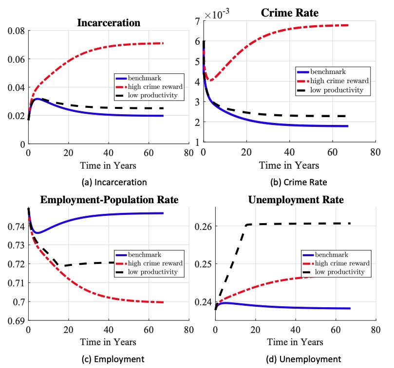
Figure 19. Other Factors: Figures a–d compare the evolution of the economy in response to the policy change and some other factors affecting the incarceration rate. The solid line plots the benchmark economy, the long dashed line plots the dynamics in response to the policy change and an increase in the mean of the crime reward distribution, and the dashed line plots the dynamics in response to the policy change and a gradual decrease in productivity
7. Conclusion
We began this paper by arguing the importance of considering dynamics driven by criminal persistence in the evaluation of punitive incarceration policy changes. We presented our argument by incorporating the theory in both a simple and a rich dynamic model. We bolstered the empirical relevance of our theory by providing both cohort and changing cross-sectional evidence consistent with the theory’s predictions relying on criminal persistence.
To quantitatively evaluate policy changes, we developed a dynamic model grounded in the Beckerian theory of rational crime in which age, human capital, and employment all deter crime. We enhanced the model with additional channels: an early life choice, criminal capital, and criminal records that segment labor markets. These additional channels enable the model to replicate salient features of criminal behavior that are important for transitional dynamics: high recidivism rates that seem to only decrease with age; and cohort dynamics after policy changes of the 1980s. Altogether we learned that luck in drawing a good crime opportunity is instrumental in the choice to enter crime and that criminal capital, particularly that gained in prison, drives criminal persistence after youth. Adding things up, most crime is done by a few individuals with long criminal records for whom pecuniary factors provide little deterrence.
The main application of the theory analyzed the impact of increased use of punitive incarceration akin to policy changes in the 1980s and arrived at three substantive conclusions. First, the change in incarceration policy on its own made a minor contribution to trends in low-skilled labor markets and a more substantive contribution to aggregate incarceration and the decline in crime. Second, the transition after a policy change follows nuanced dynamics that can take several turns over subsequent decades. Increases in incarceration initially separate the worst criminals, who also have the worst labor market prospects, from the general population. Later, the additional individuals who cycle through the prison system re-enter the population with even worse labor market prospects and higher criminality than before. Full deterrent effects are not realized until new cohorts are born under the new policy, choosing less crime and higher labor force attachment from early in life. Third, the theory uniquely predicts that crime becomes more concentrated in a smaller portion of the population who engage in crime more intensely. These changes in the extensive and intensive margins of crime mirrors empirical trends and provides further support to the validity of our theory. They also contribute to our result that increased punitive policy increases economic inequality within low-skilled populations. We spent ample time in the paper further discussing exactly what drives all three of these predictions, both qualitatively and quantitatively.
Our findings uniquely emphasize that the issue of dynamics needs to be addressed when approaching questions related to both criminal justice policy design and criminal justice policy evaluation. Policy evaluation relying on econometric inferences on policy experiments must consider that short-run effects of policy changes can run in directions that are opposite from long-run effects, as we have shown. Policy design must consider how the costs of sharp policy changes are borne unequally across cohorts. A specific prescription to be further researched is whether a less abrupt approach would be of benefit. In other words, if intensified punitive policies were announced in advance, and if such announcements were followed by gradual implementation, then perhaps welfare could be improved. This would allow a greater chance for agents to respond, potentially preventing a large increase in incarceration and collateral effects in the short term.
References
Acemoglu, D. (2002). Technical change, inequality, and the labor market. Journal of Economic Literature 40(1), 7-72.
Bayer, Patrick, Randi Hjalmarsson, and David Pozen. 2009. “Building Criminal Capital Behind Bars: Peer Effects in Juvenile Corrections.” Quarterly Journal of Economics 124 (1): 105–47.
Becker, Gary S. 1968. “Crime and Punishment: An Economic Approach.” Journal of Political Economy 76 (2): 169–217.
Bhati, Avinash Singh. 2010. “Criminal Recidivism in a Large Cohort of Offenders Released from Prison in Florida, 2004–2008.” Inter-university Consortium for Political and Social Research [distributor]. https://doi.org/10.3886/ICPSR27781.v1.
BJS and F. B. of Prisons (1974, 1979, 1986, 1991, 1997). Survey of inmates in state and federal correctional facilities. Inter-university consortium for political and social research.
Blumstein, Alfred, and Allen J. Beck. 1999. “Population Growth in US Prisons, 1980–1996.” Crime and Justice 26 (January): 17–61.
Blumstein, Alfred, and Jacqueline Cohen. 1973. “A Theory of the Stability of Punishment.” Journal of Criminal Law and Criminology 64 (2): 198–207.
Burdett, Kenneth, Ricardo Lagos, and Randall Wright. 2003. “Crime, Inequality, and Unemployment.” American Economic Review 93 (5): 1764–77.
Bureau of Labor Statistics, US Department of Labor. 2014. National Longitudinal Survey of Youth 1979 cohort, 1979–2012 (rounds 1–25). Columbus, OH: Center for Human Resource Research, Ohio State University.
Cahalan, M. and L. Parsons (Dec 1986). Historical corrections statistics in the united states, 1850-1984e. NCJ-102529.
Carson, E. A. and J. Mulako-Wangota (2017). Bureau of justice statistics tables. data retrieved from Corrections Statistical Analysis Tool (CSAT)- Prisoners, www.bjs.gov.
Caucutt, Elizabeth, G. N. and C. Rauh (2017). Is marriage for white people? incarceration and the racial marriage divide. In 2017 Meeting Papers, Number 779. Society for Economic Dynamics.
Cunniff, M. N. A. o. C. J. P. (1994). Recidivism of felons on probation, 1986-1989: [united states].
Durlauf, Steven N., Salvador Navarro, and David A. Rivers. 2010. “Understanding Aggregate Crime Regressions.” Journal of Econometrics 158 (2): 306–17.
Eisen, Lauren-Brooke, and James Cullen. 2016. “Update: Changes in State Imprisonment Rates.” Brennan Center for Justice.
Elder Jr., Glen H. 1985. Perspectives on the Life Course. Ithaca, New York: Cornell University Press.
Engelhardt, Bryan. 2010. “The Effect of Employment Frictions on Crime.” Journal of Labor Economics 28 (3): 677–718.
Engelhardt, Bryan Eldon, Guillaume Rocheteau, and Peter Rupert. 2008. “Crime and the Labor Market: A Search Model with Optimal Contracts.” Journal of Public Economics 92 (10–11): 1876–91.
Federal Bureau of Investigation. (2017). Crime in the united states. data retrieved from Uniform Crime Reporting Statistics Data Tool, https://www.ucrdatatool.gov/.
Fella, Giulio, and Giovanni Gallipoli. 2014. “Education and Crime over the Life Cycle.” Review of Economic Studies 81 (4): 1484–1517.
Freeman, Richard B. 1999. “The Economics of Crime.” In Handbook of Labor Economics Vol. 3c, edited by Orley Ashenfelter and David Card. Amsterdam: North Holland Publishers, 3529–71.
Fu, Chao, and Kenneth I. Wolpin. 2018. “Structural Estimation of a Becker-Ehrlich Equilibrium Model of Crime: Allocating Police Across Cities to Reduce Crime.” Review of Economic Studies 85 (4): 2097–2138.
Gottfredson, Michael R., and Travis Hirschi. 1990. A General Theory of Crime. Palo Alto, CA: Stanford University Press.
Huang, Chien-Chieh, Derek Laing, and Ping Wang. 2004. “Crime and Poverty: A Search-Theoretic Approach.” International Economic Review 45 (3): 909–38.
İmrohoroğlu, A., A. Merlo, and P. Rupert. 2004. “What Accounts for the Decline in Crime?.” International Economic Review 45 (3): 707–29.
James, Nathan. 2013. The Federal Prison Population Buildup: Overview, Policy Changes, Issues, and Options. CRS Report 42937. Congressional Research Service.
Kitao, Sagiri, Lars Ljungqvist, and Thomas J. Sargent. 2017. “A Life-Cycle Model of Trans-Atlantic Employment Experiences.” Review of Economic Dynamics 25 (April): 320–49.
Lagakos, David, Benjamin Moll, Tommaso Porzio, Nancy Qian, and Todd Schoellman. 2016. “LifeCycle Wage Growth Across Countries.” Journal of Political Economy 126 (2): 797–849.
Laub, John H., and Robert J. Sampson. 1993. “Turning Points in the Life Course: Why Change Matters to the Study of Crime.” Criminology 31 (3): 301–25.
Ljungqvist, L. and T. J. Sargent (1998). The European unemployment dilemma. Journal of political Economy 106(3), 514–550.
Lochner, Lance. 2004. “Education, Work, and Crime: A Human Capital Approach.” International Economic Review 45 (3): 811–43.
McCrary, Justin. 2010. “Dynamic Perspectives on Crime.” In Handbook on the Economics of Crime, edited by Bruce L. Benson and Paul R. Zimmerman. Cheltenham, UK: Edward Elgar Publishing, 82.
Nagin, Daniel, and Raymond Paternoster. 2000. “Population Heterogeneity and State Dependence: State of the Evidence and Directions for Future Research.” Journal of Quantitative Criminology 16 (2): 117– 44.
Neal, Derek, and Armin Rick. 2014. “The Prison Boom and the Lack of Black Progress after Smith and Welch.” NBER Working Paper No. 20283. National Bureau of Economic Research, Cambridge, MA.
Pettit, Becky. 2012. Invisible Men: Mass Incarceration and the Myth of Black Progress. New York: Russell Sage Foundation.
Pfaff, John F. 2012. “The Micro and Macro Causes of Prison Growth.” Georgia State University Law Review 28 (4): 1239.
Pissarides, Christopher A. 1985. “Short-Run Equilibrium Dynamics of Unemployment, Vacancies, and Real Wages.” American Economic Review 75 (4): 676–90.
Raphael, Steven, and Michael A. Stoll. 2009. “Why Are So Many Americans in Prison?” In Do Prisons Make Us Safer?: The Benefits and Costs of the Prison Boom. New York: Russell Sage Foundation, 27.
Ruggles, Steven, Sarah Flood, Ronald Goeken, Josiah Grover, Erin Meyer, Jose Pacas, and Matthew Sobek. 2018. “IPUMS USA: Version 8.0 [Dataset].” Minneapolis, MN: Integrated Public Use Microdata Series. https://doi.org/10.18128/D010.V8.0
Sampson, Robert J., and John H. Laub. 1990. “Crime and Deviance over the Life Course: The Salience of Adult Social Bonds.” American Sociological Review 55 (5): 609–27.
Schulhofer-Wohl, Sam, and Y. Claire Yang. 2016. “Modeling the Evolution of Age and Cohort Effects.” In Dynamic Demographic Analysis, edited by Robert E. Schoen. Cham, Switzerland: Springer International Publishing, 313–35.
Shimer, R. (2005). The cyclical behavior of equilibrium unemployment and vacancies. American economic review, 25-49.
Steffensmeier, Darrell J., Emilie Andersen Allan, Miles D. Harer, and Cathy Streifel. 1989. “Age and the Distribution of Crime.” American Journal of Sociology 94 (4): 803–31.
United States Department of Justice. Office of Justice Programs. Bureau of Justice Statistics. 2011. “Recidivism among Released Prisoners, 1983: [United States].” Ann Arbor, MI: Inter-university Consortium for Political and Social Research [distributor]. https://doi.org/10.3886/ICPSR08875.v3.
United States Department of Justice. Office of Justice Programs. Bureau of Justice Statistics (2013). National corrections reporting program series, 1983-2012: [united states].
United States Department of Justice. Office of Justice Programs. Bureau of Justice Statistics (2014). Recidivism among released prisoners, 1994: [united states]. Ann Arbor, MI: Inter-university Consortium for Political and Social Research [distributor].