Send Them Back? The Real Estate Consequences of Repatriations

Cortes, Gustavo; Sant'Anna, Vinicios

“The Mexican immigrant is not good material for citizenship, and in some places Mexican colonies are decidedly objectionable.” — The Washington Post, Jan 25, 1930.

“Between 40 and 50 unemployed American laborers threatened a united disturbance this morning when they tried to prevent Mexican workmen to continue their work (…) demanding that the contractors employ white labor.” — The Los Angeles Times, Oct 17, 1931.

Introduction

Immigration has consistently been at the center of the political and economic controversies in history. The economic literature has shown that migration affects local economies through various channels, including labor markets, foreign direct investment, and innovation. A growing part of this literature has focused on the impacts of migration on housing. Studying housing remains vital for at least two reasons. First, housing is an essential component of most households’ wealth and expenditure. Second, since immigrants need a house to live in, intense immigration flows can significantly affect local housing quantities and prices, potentially impacting the local wealth distribution, the cost of living, and real wages. However, most of what we know about the effects of migration on housing comes from studies that focus on the inflows of immigrants (e.g., Saiz (2003), Ottaviano and Peri (2006), Saiz (2007), Akbari and Aydede (2012), Howard (2020)).

This paper sheds light on an understudied type of migration shock to housing markets: an out-migration shock. Making this distinction when studying housing markets is indispensable because housing investment is naturally irreversible. Once a dwelling unit is built, it is prohibitively expensive to convert it back to investable capital—a characteristic also known as the putty-clay nature of real estate investment.¹ The existing literature shows evidence that in-migration shocks to a city are likely to increase the demand for housing, inducing the construction of new house units (Howard (2020)). However, the empirical literature is silent on how an out-migration shock affects house prices, rents, and construction activity.

Because housing is durable, asymmetric effects on prices may arise, making us incapable of drawing precise conclusions about out-migration episodes from in-migration elasticities. Potentially, one would expect a larger impact on prices in the short run due to the inelastic downward nature of housing (Glaeser and Gyourko (2005)). Precisely gauging these impacts is one of our contributions.

This gap of out-migration studies in the housing literature has become more critical as we observe the invigoration of national-populism and immigration backlash across the globe. In recent years, influential leaders have voiced strong views against immigration in election campaigns and electoral mandates.² Following this rhetoric, immigration policy has also been shifting towards stricter actions.³ While most immigration policies are designed to curb the inflow of immigrants (e.g., by limiting the entrance of immigrants from specific countries), more extreme actions involving the mass expulsion of immigrants through raids and deportations have also become frequent in politicians’ speeches.⁴

Our paper studies one of the largest ethnically motivated migration shocks in US history to study the impact of out-migration on local housing. Specifically, we study the United States’ Mexican repatriation of the 1930s—a negative, large-scale shock to the Mexican workforce in the US—to quantify its effects on housing prices and real estate outcomes of US cities. Between 1930 and 1936, organized labor movements, press, and local governments harassed, pressured, and forced Mexicans to leave the US (Hoffman (1974); Guerin-Gonzales (1994); Sánchez (1995); Balderrama and Rodríguez (2006); Enciso (2017); Lee, Peri and Yasenov (2022)).⁵ We use data from the US Censuses of 1930 and 1940 to assess whether and how housing-market conditions in local economies were affected by the intensity of the repatriation.⁶ The broad presence of Mexicans in the US labor force and their dispersed geographical distribution across the US territory allows us to exploit the substantial variation in the repatriation of Mexicans across US cities.

There are key empirical challenges in estimating the housing effects of out-migration. The nature of the Mexican repatriation as an out-migration shock allows us to address at least two common challenges. First, most out-migration episodes occur in response to wars or natural disasters (e.g., Boustan, Kahn, Rhode and Yanguas (2020)). Obviously, these events destroy the existing supply of houses and affect real estate markets through channels other than just out-migration. As an ethnically motivated shock to out-migration rather than an armed conflict or natural catastrophe, the Mexican repatriation is less likely to induce the immediate destruction of housing units. Second, the business cycle conditions can directly affect the housing markets while also affecting immigrants’ decisions to move. The potential simultaneity between the migration flows and the local economic conditions can lead to biased estimates of the economic consequences of immigration. Because the Mexican repatriation involved harassing, pressuring, and forcing targeted individuals of a specific nationality to leave the country, it likely caused Mexicans to out-migrate for reasons beyond economic adversity. This helps to mitigate the usual confounding effects that are a common concern in the literature. We, therefore, approach the Mexican repatriation as a unique setting to evaluate the costs and benefits of out-migration for its ability to address these empirical challenges.

Nonetheless, the intensity of the repatriation efforts could be correlated with other city characteristics that might affect housing markets. To isolate the Mexican repatriation effects on real estate, we employ an instrumental variable (IV) approach. Our instrumental variable exploits patterns in the road infrastructure of 1930, combined with the historical presence of Mexican immigrants in the US at the turn of the century. More specifically, it combines a measure of exposure to the out-migration shock (the share of Mexican workers in 1900) with a measure of the cost of repatriating workers (travel distance based on the US road infrastructure in 1930). Our baseline specifications also include a series of control variables, including state fixed effects and sector employment shares to account for heterogeneous exposure to the Great Depression.⁷

Considering the nature of the Mexican repatriation as a local shock due to out-migration of a specific part of the population, we begin by investigating its effects on prices of Mexican-occupied houses. We develop a novel automated matching technique to link addresses across the 1930 and 1940 Censuses from the IPUMS Restricted Complete Count Data (Ruggles, Fitch, Goeken, Grover, Hacker, Nelson, Pacas, Roberts and Sobek (2020a)). The matched address sample allows us to track each housing unit’s value or rent evolution across the two censuses. Using this sample, our two-stage least squares (2SLS) estimates show that the Mexican repatriation had a strikingly large and persistent effect on houses where Mexicans lived in 1930. We find that the value of houses inhabited by Mexicans in 1930 devalued by an average of 8.2 percentage points between 1930 and 1940 for every percentage point drop in a city’s Mexican population. Rents on houses occupied by Mexicans in 1930 also fell by more than 2 percentage points for every percentage point of Mexican outflow. To illustrate the economic significance of this effect, we compare it to the median devaluation of Mexican-occupied houses in the period. The median house owned by Mexicans devalued by 41% between 1930 and 1940. This means that the partial negative effect of the repatriation on Mexican-owned houses is equivalent to one fifth (8.2/41 = 20%) of the decline observed in the median Mexican-occupied house value in our sample. The value of the median rent paid by Mexicans fell by 33% between 1930 and 1940. For rented units, the partial effect of the repatriation is equivalent to six percent (2/33 = 6%) of the decline observed in the median rent of Mexican-occupied houses in our sample. More importantly, despite the large devaluation of Mexican-occupied houses, we do not find evidence of strong effects on prices of US-born occupied housing in those cities.

Next, we study what happened to the resident composition of the Mexican-occupied houses in 1930. Using the matched address sample, we find that houses previously owned by Mexican immigrants decreased the number of Mexican residents in response to the repatriation. We do not find strong evidence supporting the inflow of US-born residents into these houses in response to the repatriation. The results of Mexican-rented houses are different. We find suggestive evidence that the repatriation increased the segregation between Mexican immigrants and US-born residents in the rented units. Our results suggest that Mexican-rented houses became less mixed with US-born residents during the period in response to the repatriation.

Given the large effects of the repatriation on Mexican-occupied housing, one natural question arises. To what extent the Mexican repatriation mattered to each city’s housing market? Using an instrumental variable approach, we turn to examine the effects of Mexican repatriation exposure on the growth rates of city-level housing market outcomes. In our baseline estimation, we find that cities with greater exposure to the Mexican repatriation faced reduced growth rates in all our housing outcome variables. Precisely, we find that a one standard deviation (1 percentage point) larger repatriation depressed the median house price growth rate (by –1.2 percentage points) and the median rent growth rate (by –1 percentage points).

We can compare these results to the observed growth rates of median house values and rents in the period to put these results into perspective. On average, median house values decreased 43.2% while median rents decreased 30.6% in the decade.

Therefore, a one standard deviation increase in exposure to the Mexican repatriation explains approximately 2.8% and 3.3% of the average decrease in house values and rents, respectively.

We also find that the repatriation depressed the growth rates of investment measures based on building permits. We find that a one standard deviation (1 percentage point) larger repatriation had lower growth rates for both the number (–13.3 percentage points) and the value (–3.7 percentage points) of building permits between 1930 and 1940. Slower growth in these outcomes suggests that the repatriation negatively impacted the expectations of future housing market conditions and local real estate activity, such as the construction of single-family homes and commercial buildings.

To illustrate our housing market findings, we compute a quasi-counterfactual exercise. We calculate the predicted growth rates for different housing-market outcomes in US cities in a hypothetical scenario where the Mexican repatriation never occurred. Assuming a simplified counterfactual outflow of Mexicans from our first stage regressions and ignoring general equilibrium effects, we predict that the growth rates would have increased substantially. For example, in Los Angeles, the value of building permits between 1930 and 1940 decreased 0.41%. Absent the repatriation, we predict that the value of building permits in Los Angeles would have fallen at a smaller rate, 0.25%. This difference was equivalent to over 100 thousand US dollars in 1930 terms.

One of the main concerns of our analysis is whether our results reflect other shocks that US cities experienced at the time. To mitigate these concerns, we conduct a series of robustness and validation tests. First, we test for an association between the instrumental variable and different measures for the intensity of the Great Depression. We conclude that the instrumental variables are not linearly associated with the adverse economic conditions that defined the Great Depression, supporting the validity of the exclusion restrictions. Second, we test for the association between the instrument and the outflow of immigrants from other nations. We find no evidence of a linear association between the instrumental variables and other immigrants’ outflow rates. Using an event study specification, we find no evidence of pre-trends in housing-market outcomes associated with the share of Mexicans in 1930.

Another concern is whether the Mexican repatriation had a direct effect on the supply of housing. In 1930, approximately 12.7% of Mexican immigrants worked in the construction or construction-related, durable goods manufacturing sectors (See Table B.3 in Appendix B for details on the employment of Mexican workers by industry in 1930). We find that the Mexican repatriation reduced the employment of Mexicans in construction and that US-born increased their employment in construction proportionally. However, the repatriation did not have a significant effect on the overall employment in the construction sector. These results suggest that, while the repatriation induced substitution of Mexicans by US-born workers in the construction and construction-related sectors, the overall employment growth in these sectors stagnated.

Related Literature. Our paper contributes to several branches of the extensive literature on the economic consequences of immigration. Within this broad literature, this paper is related to the literature that studies the economic consequences of forced migration.⁸ Most studies have focused on the assessment of the economic effects on receiving regions (Hornung (2014); Schumann (2014); Johnson and Koyama (2017)). In contrast, this paper provides evidence of the economic consequences of forced migrations to origin regions. This is closely related to Chaney and Hornbeck (2016); Testa (2020); Ferrara and Fishback (2020), who study politically or ethnically motivated expulsion events in history. While these papers show evidence of depressed regional growth or development from sending regions, our paper is the first to directly quantify the effects of an ethnically motivated out-migration shock on housing prices, one of the channels through which migration can affect economic growth.

Our paper relates to the recent literature that focuses on the economic effects of restrictions to immigration based on race or country of origin (e.g., Clemens, Lewis and Postel (2018); Abramitzky, Ager, Boustan, Cohen and Hansen (2020); Feigenberg (2020); Tabellini (2020); Lee, Peri and Yasenov (2022)). In studying the economic consequences of the 1930s Mexican repatriation, our analysis closely relates to Lee, Peri and Yasenov (2022), who study the labor market consequences from the repatriation. The authors find that in the regions more exposed to the repatriation, the US-born workers faced a smaller probability of having a job in 1940, and that this effect was larger to low-skilled workers. The authors also find that the repatriation did not cause internal migration of US-born workers to replace the repatriated immigrants.

Our analysis contributes to their findings by studying the effects of the Mexican repatriation to housing markets in the US. We use real estate conditions to gauge the costs to local economic growth because housing is a crucial channel through which immigration affects economic activity. Moreover, the recent Great Recession has drawn fresh attention from scholars to the housing sector and its responsiveness to immigration shocks.

A growing strand of the literature looks specifically at the effects of migration shocks on housing markets (Saiz (2003), Greulich et al. (2004), Ottaviano and Peri (2006), Saiz (2007), Akbari and Aydede (2012), Alix-Garcia, Bartlett and Saah (2012), Gonzalez and Ortega (2013), Mussa et al. (2017), Depetris-Chauvin and Santos (2018), Howard (2020)). In dealing with the challenge in identifying the causality of migration effects, the existing literature typically uses exogenous shocks of inflows of migrants to a region to study the effects on house prices and availability. Most studies find that immigration increases rents and house prices, suggesting that immigrants do not entirely displace natives. Few studies focus on the effects of forced migration on housing. For instance, Alix-Garcia, Bartlett and Saah (2012) and Balkan, Tok, Torun and Tumen (2018) study the economic effect of displaced populations on housing, focusing on the effects of receiving regions. Our paper contributes to this literature by assessing the effects of out-migration on the sending regions.

This paper also relates to the literature studying populism and nationalism, primarily focusing on 1930s America (Bennett (1969)). Recent work has focused on the direct consequences of exposure to populist radio hosts on political preferences (Wang (2021)) or the effects on uncertainty caused by populist politicians’ actions (Mathy and Ziebarth (2017)). As Tabellini (2020) shows, immigration can trigger strong political backlash resulting in more conservative, anti-immigrant policies. Therefore, our paper contributes to understanding the economic consequences of immigration backlash rooted in the ideals of national-populism. Our findings are particularly relevant to today’s ongoing debate on the economic effects of immigration backlash. Our results show that repatriations have large impacts on house values and rents of more exposed neighborhoods and that these effects matter to city-level housing in terms of coincident and leading housing indicators.

Mexican Immigration in the 1920s and the 1930s Repatriation

The US experienced a massive inflow of immigrants in the late 19th century and the early 20th century, especially from Europeans escaping adverse conditions in their home countries.⁹ Mexican immigration grew steadily throughout the early decades of the 20th century, but especially during the 1920s. This robust inflow was mainly driven by US employers recruiting Mexican workers in agriculture, railroad, meatpacking, and steel mill sectors. In the 1920s, the number of Mexican immigrants increased dramatically. The increased demand for cheap labor coincided with the 1924 Immigration Act, which imposed quotas on European immigration (Abramitzky, Ager, Boustan, Cohen and Hansen (2020)), which made many employers turn to Mexican labor to fill the job vacancies. The pressing economic conditions and armed conflicts in Mexico, such as the Mexican Revolution (1910–1920) and the Cristero War (1926–1929), also contributed to the inflow.

As the US economy entered the Great Depression, starting with the 1929 Crash, organized groups including labor unions, local authorities, and local media pressed for immigration quotas and repatriation of Mexicans.¹⁰ As the Depression deepened, many Americans began to view Mexicans as unwelcome aliens who were a burden on their local community. The historiography argues that the Mexican community was an easier target for two main reasons. First, the number of Mexican immigrants had increased dramatically in the previous years, making them the largest group of newcomers in many cities in the US. Second, because of ethnic and cultural differences, some Americans often saw them as unassimilable, that is, unable to become a part of American culture and society (Simon (1974), Balderrama and Rodríguez (2006), Enciso (2017)).

The local and decentralized nature of the Mexican repatriation makes it challenging to determine the exact number of repatriated individuals. This uncertainty explains the variation among historians’ estimations of the total Mexican outflow in the 1930s.¹¹ The more conservative estimates by Hoffman (1974) and Gratton and Merchant (2013) suggest that nearly 400,000 Mexicans left the US between 1929 and 1937, while Balderrama and Rodríguez (2006) cite a much larger number—from 1 million to 2 million, based on estimates that attempt to include those undocumented immigrants omitted from official calculations.

Using the Census, we calculate that there were 263,900 fewer Mexican immigrants in the US in 1940 than in 1930, which constituted 33.2% of the overall Mexican population present in the US as of 1930.¹² Figure 1 depicts the surge of Mexican-born immigrants between 1900 and 1920, followed by a sharp decline between 1930 and 1940. Another interesting fact from Figure 1 is that the number of immigrants from other (non-Mexican) Latin American countries did not decline in the same period.

Figure 1. Total Latin American immigrant population in the United States by origin (1880–1960).

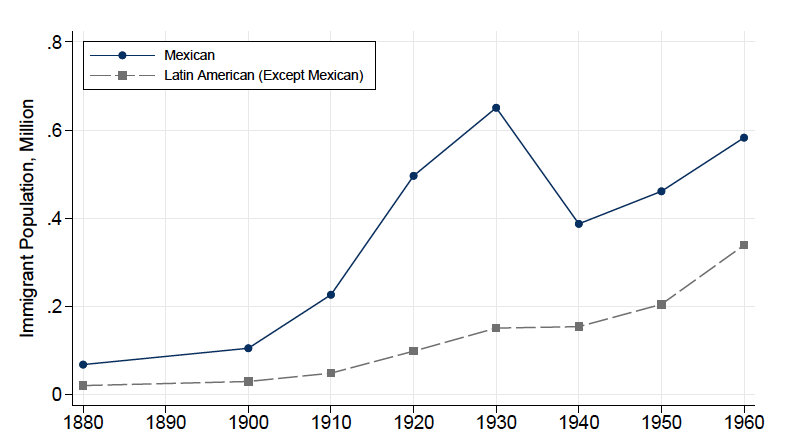
This figure shows the total number of Mexican and other Latin American immigrants in the United States from 1880 to 1960. Immigrants are defined according to the country of birth reported on each census. Latin American countries include Central America (Belize/British Honduras, Costa Rica, El Salvador, Guatemala, Honduras, Nicaragua, and Panama), the Caribbean (Cuba, Dominican Republic, Haiti, Jamaica, Antigua-Barbuda, Bahamas, Barbados, Dominica, Grenada, Montserrat, St. Kitts-Nevis, St. Lucia, St. Vincent, Trinidad and Tobago, Turks and Caicos, British Virgin Islands, Netherlands Antilles, Curacao, Guadeloupe, and St. Barthelemy), and South America (Argentina, Bolivia, Brazil, Chile, Colombia, Ecuador, Guyana/British Guiana, Paraguay, Peru, Suriname, Uruguay, and Venezuela).

While the existing historiography varies in their accounts of the period, there is a consensus that coercion, forced deportation, and various other fear-spreading tactics were used extensively against the Mexican population of the time. The historical accounts of this period documents that local authorities encouraged and enforced repatriation, even though it was officially categorized as voluntary migration (Valdés (1988); Balderrama and Rodríguez (2006)). Immigration officers and local police sometimes assisted welfare agencies and even staged raids to convince Mexicans to depart. They harassed Mexicans, provided free transportation in trains, and—at least partially—coerced them to leave their US homes.

In Internet Appendix Figure A.1, we present historical newspaper evidence of anti-Mexican sentiment and hostile acts targeted at Mexican immigrants. These acts involved the government (e.g., immigration officers), organized labor (e.g., unionized workers), and the press (e.g., local and national newspapers). As shown in Panel A, The New York Times reported in 1931 that 35,000 Mexican immigrants in California were “pressed by economic diversity, fearful over recently renewed activities of immigration authorities, and perplexed by what they regard as anti-Mexican sentiment.” This illustrates that economic distress (“idleness”) and tighter enforcement from government immigration officials played an essential role in Mexicans’ decision to leave the country.¹³ In Panel B, the Los Angeles Times reports a near-riot in 1930 in which some 50 unemployed American laborers “tried to prevent Mexican workmen (…) to continue their work by guarding their toolboxes and demanding that the contractors employ white labor.” The national and local press also contributed to the negative climate by publishing articles and opinions demeaning to Mexican immigrants. For example, as shown in Panel C, The Washington Post argued that “the Mexican immigrant is not good material for citizenship, and in some places Mexican colonies are decidedly objectionable,” even though it conceded that, given the economic importance of Mexican immigrants, “a sudden reversal of [immigration] policy would work great hardship to employers in the Southwest.”

Figure 2. Geographical distribution of the inflow and outflow of Mexicans.

(A) Mexican Inflow (1920–1930)

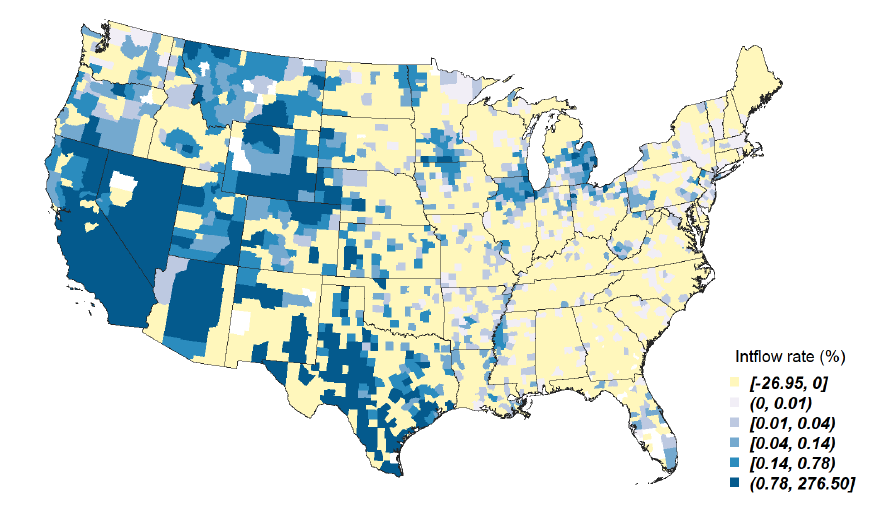
(B) Mexican Outflow (1930–1940)

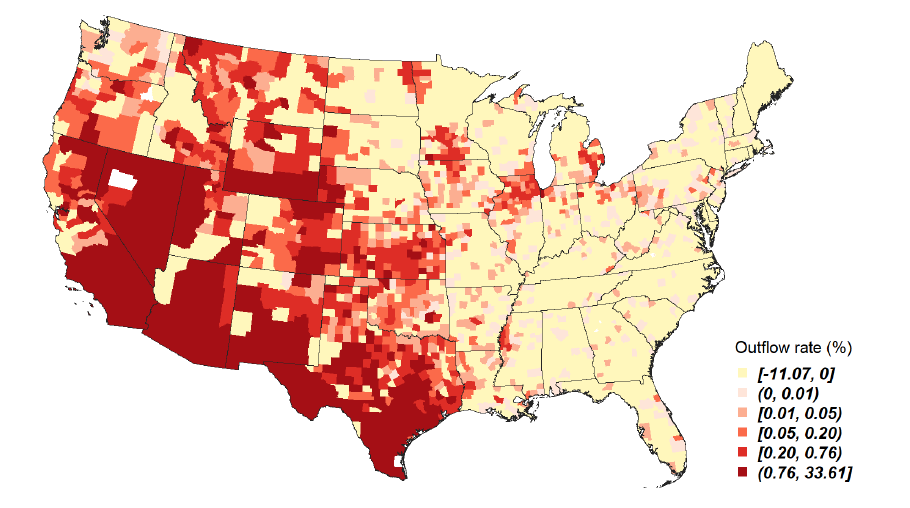
This figure shows, for each county, the 1920-30 inflow (Panel A) and the 1930–40 outflow (Panel B) of Mexicans as calculated from the full-count US Censuses of 1920, 1930, and 1940. The nationalities are defined based on the person’s place of birth from the US Census. The flows are measured by the Mexican working-age population’s county-level change relative to the local working-age population. For instance, a Mexican outflow of 10% means that the drop in the Mexican population of that county is equivalent to a 10% drop in the total working-age population. We define counties according to 1930 limits by IPUMS-NHGIS (Manson et al. (2020)).

Figure 3. Positive correlation: repatriation intensity versus Mexican population shares from 1900.

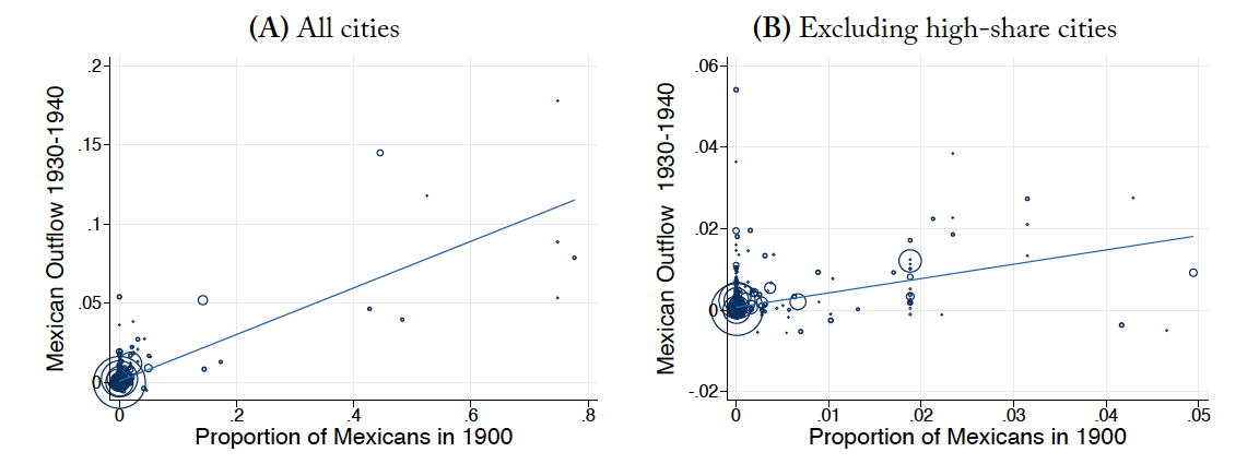
This figure shows the positive correlation between Mexican Outflow (defined in Equation (2)) and the county level share of Mexicans in 1900, i.e., before the repatriation shock. Panel A presents the scatter plot for all cities in our sample, and Panel B repeats the scatter plot after excluding cities with more than 5% share of Mexicans in 1900.

The lack of granular data on the individual US-Mexico border crossings during that time makes it challenging to determine the exact importance of these repatriation efforts to the overall Mexican outflow. The available estimates in the literature suggest that the repatriation efforts involving harassment, coercion, pressures, and forced deportations were the primary determinant of the Mexican outflow of the 1930s. For instance, using the outflow of French-Canadian immigrants as a comparison group, Gratton and Merchant (2013) estimate that over 70% of the observed net Mexican outflow was not voluntary, due to excess repatriation.

We next document the geographic distribution across US counties of Mexican immigration before and after the repatriation. Panel A of Figure 2 presents the inflow as measured by the change in the total number of Mexicans between 1920 and 1930 as a share of each county’s total working-age population. Darker blue shades represent higher inflows. Conversely, Panel B of Figure 2 portrays counties with a greater outflow of Mexicans between 1930 and 1940 with darker shades of red.

Overall, counties with larger Mexican populations also experienced higher outflow rates in the 1930s. We present this correlation more clearly in Panel A of Figure 3, which shows a strong linear relationship between the 1900 Mexican population share and the 1930–1940 outflow of Mexicans. Although inflows and outflows were more substantial in counties near the border with Mexico, they were quite widespread. We observe counties with considerable migration flows in the West (Oregon, Nevada, Washington), the Midwest (Illinois, Indiana, Michigan, Ohio), and the East (Pennsylvania). If we exclude border cities and redo the scatter plot in Panel B of Figure 3, we see that the strong relationship remains for cities throughout the entire geographic span of the continental US, as documented by Balderrama and Rodríguez (2006).

A helpful way to put the Mexican repatriation in perspective is to compare the outflow rates of Mexicans and immigrants from other ethnicities. Figure 4 examines the change in the US working-age population before (in dark blue) and after (in gray) the repatriation period for different ethnic groups. It shows that the massive Mexican outflow of almost 40% during the 1930–1940 period is unmatched by other groups. Their outflow is nearly twice that of the Europeans. Canadians—who also share a border with the US and could return more easily than other nationals—have half of the outflow rate. A final takeaway from Figure 4 is that non-Mexican Latin American immigrants experienced a substantially smaller outflow—even though the inflows of both Mexican and non-Mexican Latin immigrants had both grown at similar percentage rates in the previous decade.

Figure 4. Percent changes in working-age population by origin: 1920–30 versus 1930–40.

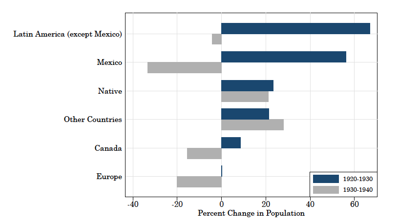
This figure shows the inflow (1920–30) and outflow (1930–40) of immigrants. The nationalities are defined based on the person’s place of birth from the US Census. For example, between 1920 and 1930 the Mexican population in the US increased by around 60%, whereas about 30% left the US in the following decade (1930–40). See notes on Figure 1 for a list of countries included under Latin America.

Empirical Strategy

Identifying the Effect of the Mexican Repatriation

The objective of our baseline empirical work is to study how the 1930s Mexican repatriation affected the evolution of housing prices in the United States. In doing so, our goal is to isolate the effect of the ethnically motivated out-migration shock from any other factor associated with housing markets. A naïve attempt to assess the relationship between the repatriation and housing price changes would be to estimate the following regression:

(1) $\begin{equation*} \Delta Y_{1930:40} = \alpha + \beta \cdot O^{MEX}_{c,1930:40} + \epsilon, \end{equation*}$

where $\Delta Y_{1930:40}$ is the percentage change of a housing market outcome between 1930 and 1940. $O^{MEX}_{c,1930:40}$ is the outflow of Mexican workers in city c in the same period. Following Lee, Peri and Yasenov (2022), we define the city-level measure of Mexican outflow from city c between 1930 and 1940, $O^{MEX}_{c,1930:40}$ :

(2) $\begin{equation*} O^{MEX}_{c,1930:40} = - \left( \frac{Pop^{MEX}_{c,1940} - Pop^{MEX}_{c,1930}}{Pop_{c,1930}} \right), \end{equation*}$

where $Pop^{MEX}_{c,t}$ is the Mexican working-age population in city c in year t (1930 or 1940), and $Pop_{c,1930}$ is the total working age population in city c in 1930.¹⁴ Because the repatriation comprises a decline in the population of Mexican workers, we multiply the growth rate by minus one for a more straightforward interpretation. ¹⁵

The main drawback of estimating Equation (1) is that, even after controlling for observable characteristics, migration flows might be correlated with other local economic conditions. The main concern is that the intensity of the Mexican repatriation might have been correlated with other local economic conditions, such as the intensity of the Great Depression, that could have influenced the evolution of housing markets between 1930 and 1940. Therefore, our empirical strategy uses an instrumental variable (IV) approach to solve the potential endogeneity between the Mexican outflow and the housing market outcomes and produce causal estimates.

Our instrumental variable combines the infrastructure of the US road network and the historical presence of Mexican immigrants in a county at the turn of the century. The relevance condition of our IV is given by the historical evidence that the repatriation was more likely to happen in counties with larger pre-existing Mexican communities (see Figure 3). To avoid contemporaneous confounders, we opt to use the share of the Mexican population in a US county in 1900 as an ex-ante measure of exposure to the repatriation.¹⁶

This has at least two advantages. First, it is less likely that the 1900s Mexican population share in a county is correlated with the economic fundamentals of the Great Depression in the 1930s. Second, for historical and cultural persistence reasons, the 1900 share is still sufficiently correlated with the size of the Mexican population in 1930, and therefore, with the population potentially exposed to the repatriation.

The transportation infrastructure also had an essential role in the repatriation. The historical evidence shows that the existing highways and railroad trackage governed the migration pathways between Mexico and the United States. As documented by Hoffman (1974), the infrastructure of the years before the Great Depression funneled travelers to the US-Mexico main border crossing stations in Texas (El Paso; Brownsville; Laredo), Arizona (Nogales; Douglas), and California (Calexico). We use novel data on county-to-county travel times in 1930, constructed by Morin and Swisher (2016) using the United States’ road network. Specifically, we define $\textit{Proximity to Mexico}_{cty,1930} = {1}/{Travel\ Time_{1930}(County, Station)}$ , where $\textit{Travel Time}$_{1930}(County, Station)$ is the travel time by roads between the county and the closest chief border crossing stations. The instrumental variable is defined as:

(3) $\begin{equation*} IV_{cty} = \textit{Proximity to Mexico}_{cty,1930} \times \left( \frac{Pop^{MEX}_{cty,1900} }{Pop_{cty,1900}} \right). \end{equation*}$

The first term, $\textit{Proximity to Mexico}_{cty,1930}$ is negatively associated with the cost of repatriation to Mexico because it was easier and cheaper to encourage (or force) repatriation if people could reach one of the crossing stations more quickly.¹⁷ The second term captures the share of Mexicans workers in a county in 1900. It is positively related to the share of the Mexican population in 1930, given the persistence of migrant networks; hence this term is correlated with the size of population “at risk” of repatriation.

With this instrumental variable at hand, we conduct the analysis in two parts. In the first part, we investigate the effects of the Mexican repatriation on the house level, particularly focusing on Mexican-occupied housing, which are more exposed to the out-migration shock, and which we expect to observe the largest effects. This allows us to precisely estimate the repatriation effects on the most exposed neighborhoods within each city. The second part of the analysis focuses on the more aggregate effects of the repatriation. The goal is to assess to what extent the Mexican repatriation mattered to city-level housing markets. The following section describes the data employed in the paper, including the matched address sample used in the house level analysis and data used to measure migration flows, housing outcomes, and other city characteristics.

Data Sources and Descriptive Statistics

Linked Address Sample. A challenge to study the Mexican repatriation’s impact on housing is the lack of data measuring the evolution of house prices at the house level. In this paper, we develop a novel automated matching technique to link addresses across the 1930 and 1940 Censuses from the IPUMS Restricted Complete Count Data (Ruggles, Fitch, Goeken, Grover, Hacker, Nelson, Pacas, Roberts and Sobek (2020a)). The address-matched sample allows us to track the evolution of each housing unit’s house values, rents, and resident composition across the 1930 and 1940 censuses. Our goal is to create a sample of housing units that we can observe both in 1930 and 1940 to assess the effect of the Mexican repatriation on its prices and residents. We propose an automated matching technique to link identifiable addresses from the two censuses. Our matching procedure relies on matching addresses based on the state, city, street name, and house number, which is described in more detail in Appendix C.

Our full 1930–1940 matched address sample contains 4.03 million linked addresses spanning over 900 US cities.¹⁸ We perform a series of sample restrictions. In studying the effects on house values and rents, we exclude the addresses that report both an owner and a renter or changed ownership status from 1930 to 1940. We also exclude households with more than 10 members to avoid outliers and transcription errors. We obtain the percentage change in house value and rents from the self-reported values in the census between 1930 and 1940. In addresses with multiple households, we aggregate this information to the address level using the median house value and the median rent reported by the households living in the same address. Finally, we obtain a sub-sample by keeping only the addresses in states with a sufficiently large Mexican population. More specifically, we restrict the analysis to states that contained a share of Mexican workers greater than 0.25% of the total state workforce living in urban areas: Arizona, Texas, California, New Mexico, Kansas, Colorado, Wyoming, Utah, Idaho, Nebraska, Indiana.

We collect information about the percentage change in house values, percentage change in rents, the average age of residents, the total number of residents, and variables that contain the racial and ethnic composition of the residents: the share of Mexican, the share of US-born white, the share of US-born black, the share of foreign-born other than Mexican, and the share of US-born residents.

Table 1 presents the summary statistics of these variables and compares them across full-count 1930 Census data (column 1), the full address-matched sample (column 2), and the two sub-samples for states more affected by the Mexican repatriation (columns 3 and 4). When comparing the full data with our matched sample, we conclude that, on average, the dwelling characteristics are quantitatively similar across the two datasets. Our matching procedure seems to favor houses with larger shares of white or US-born residents, or houses owned in 1930. The variables on the average house value and rents are similar for the two samples. When comparing the state-restricted samples (columns 3 and 4), we observe larger shares of Mexican residents and smaller shares of US-born residents. We also observe smaller house values and rents due to the sample restrictions.

Table 1. House-level descriptive statistics.

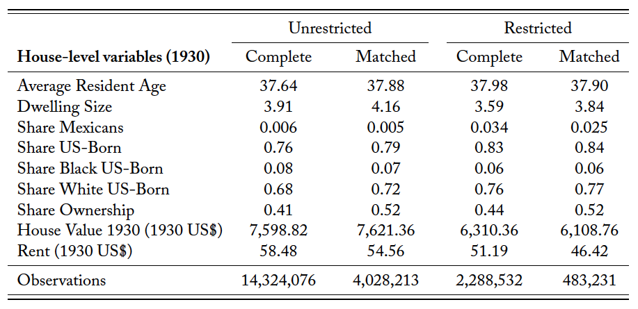
This table presents the mean statistic for variables obtained at the house level. Average Resident Age is the average age for all working-age residents within the same address in the 1930 Census. Dwelling Size reports how many persons lived within the entire dwelling in 1930. Share Mexicans is the number of working-age Mexican immigrants in any given address as a share of the total number of working-age residents in that same address. Similarly, Share Black US-born, Share White US-born, and Share US-Born are the shares of black, white or total US-born residents in an address, respectively. These measures are constructed using the information of race and place of birth of each resident from the 1930 Census. Share Ownership indicates the share of residents that were house owners in any given address. In studying the changes in house values and rents, we exclude from the sample addresses that report both an owner and a renter or changed ownership status from 1930 to 1940. House Value and Rent are the self-reported house value and rent in 1930 US dollars, respectively. For addresses with multiple households, we aggregate this information using the median house value and the median rent reported by the households in the same address. The table below presents the summary statistics of these variables and compare them across complete-count 1930 Census data (column 1), the full address-matched sample (column 2), and the equivalent complete (column 3) and matched (column 4) samples when restricting to states that contained a share of Mexican workers greater than 0.25% of the total state workforce in the studied cities: Arizona, Texas, California, New Mexico, Kansas, Colorado, Wyoming, Utah, Idaho, Nebraska, Indiana.

City Demographics, Immigration, and Economic Activity. To obtain measures of cities’ economic and demographic characteristics, we use data from 868 US cities that we can consistently identify in the 1930 and 1940 full-count US Censuses (Ruggles, Flood, Goeken, Grover, Meyer, Pacas and Sobek (2020b)).¹⁹ The censuses provide the information used to construct our main variables to measure immigration flows.²⁰ They also provide information on economic and demographic characteristics used as controls in our estimations. The baseline control variables include the Average Age, average School Attendance, share of Unemployed workers, which consists of the city-level averages of the worker’s age, school attendance status, and share of unemployed workers among the working-age population.

We refer to this set of control variables as baseline controls. Average Age and School Attendance are important to control for the characteristics of the working-age population in each city. The share of Unemployed workers and employment Sector Shares aim to capture the effects of the Depression on housing market outcomes across cities within each state. The unemployment share captures the economic conditions of cities in 1930, while sector shares account for heterogeneous effects of the Depression associated with the sector composition of cities.

As additional controls, we also use geographical and economic variables from the county-level dataset assembled by Fishback, Horrace and Kantor (2005), and Hornbeck (2012). In the 1930s, the Dust Bowl was a natural disaster that caused hardship in rural American states and induced migration out of the affected areas (Hornbeck (2012, 2021)). To measure and control for the exposure of a county to the Dust Bowl, we use the months of severe drought interacted with the share of farming land to measure the impact on a county of the Dust Bowl from Fishback, Horrace and Kantor (2005) and the fraction of each county exposed to medium and high permanent soil erosion from Hornbeck (2012). From Fishback, Horrace and Kantor (2005), we also use their county-level retail sales growth between 1929 and 1935 as a proxy for consumption and economic activity. We use the log of the median house value in 1930 as an additional control to capture for the contemporaneous conditions of the housing market.²¹

City-level outcome variables. To study the consequences of the Mexican repatriation on city-level housing market outcomes, we use the information on house prices from the US Census and aggregate it to the city-level. The 1930 and 1940 Censuses include the self-reported values of housing units and rents in nominal US dollars. To reduce outlier influence when averaging out self-reported variables, we calculate the median house value and rent in each city from the working-age population not living in group quarters. In some specifications, we also consider alternative percentiles of the within-city house value and rent distributions. We convert nominal values to real 1920 US dollars using the Consumer Price Index from the Federal Reserve Bank Database (FRED) of the St. Louis Federal Reserve Bank.

We use the number and value of building permits as additional indicators of city-level housing and construction activity. Building permits must be filed with local authorities before any construction can take place. We consider two types of building permits.

The first is the total value of building permits, taken from issues of Dun & Bradstreet’s Review, a well-known business and financial publication in the 1920s and 1930s.²² The value of building permits represents the cost of new commercial and residential buildings for 215 cities across the US. The building permit figures represent estimated building costs under permits issued to prospective builders within the corporate limits of the cities. They include new residential and non-residential buildings, and additions, alterations, and repairs, excluding land costs. The data are compiled from reports furnished monthly to Dun & Bradstreet, Inc. by the building departments of the various cities.

The second series on building permits is the number of building permits collected by Snowden (2006) from issues of the Bulletin of the Bureau of Labor Statistics. These permits refer to single-family houses authorized for construction in 250 cities.

The building permit number series thus more closely reflects housing activity, whereas the building permits values are likely dominated by commercial and business construction. This fundamental difference in the construction of these series lets us consider both types of construction activity. However, it comes at the cost of precluding us from calculating a building permit-based price index (e.g., dividing the value by the number of building permits). We, therefore, rely on the Census’ median house value as our primary variable proxying house prices.

Descriptive Statistics. Table 2 presents sample summary statistics. All growth rates and share variables are presented in percentages. We can see that the average city experienced a decrease in the Mexican population equal to 0.2 percent of the city’s total population. There is substantial heterogeneity. San Benito and El Paso in Texas experienced the two greatest outflows. By 1940, they had lost Mexican population, equivalent to 17.8% (San Benito) and 14.5% (El Paso) of their total population. East Chicago, Indiana, part of Chicago’s commuting zone, was the seventh most affected city. As the East Chicago example shows, some cities distant from the Mexican border felt a measurable effect of the Mexican repatriation.²³ States on the list of top 10 of the most affected cities include Texas, California, Indiana, and Arizona.²⁴ Figures B.1, B.2, B.3, and B.4 in the Internet Appendix illustrate the geographic span of our housing variables with maps that show the series of building permits (number and value), median house values, and median rents for US cities. Despite the smaller number of cities shown in the building permits maps, our samples span a significant share of the US territory, accounting for the most populated and economically relevant cities in that period.

Table 2. City-level descriptive statistics.

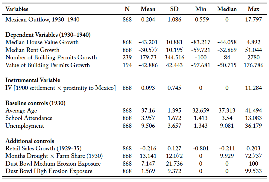
This table presents summary statistics for variables used in our empirical analysis. Mexican Outflow is constructed in Equation (2) and is the city-level change in the Mexican labor force between 1930 and 1940 divided by the city’s total working-age population in 1930. The dependent variables (growth in the number of building permits, growth in the value of building permits, growth of the median house value, and growth of median rent are the main city-level real estate market outcomes studied in our regressions and are described in detail in Section 3.2. Section 3.1 describes the construction of our instrumental variable, which combines the proximity to the Mexican border (calculated using travel times in 1930 throughout the US road network to the nearest Mexican border crossing station) interacted with the historical Mexican settlements (share of Mexican immigrants in 1900). The baseline control variables are from the 1930 Census and consist of the city-level averages of the worker’s age, school attendance status, and share of unemployed workers. We use as an additional control variable the county level retail sales growth (a measure for the Great Depression intensity) from Fishback, Horrace and Kantor (2005). We also control for the intensity of the Dust Bowl environmental catastrophe using county-level measures for months of drought interacted with the county’s farm land share from Fishback, Horrace and Kantor (2005), and the fraction of each county exposed to medium and high permanent soil erosion during the 1930s from Hornbeck (2012). Our full sample contains 868 US cities.

The 1930s Mexican Repatriation and Housing

Effects of the Repatriation at the House Level

Considering the nature of the Mexican repatriation, a local shock due to out-migration of a specific part of the population, it is plausible to expect that regions within a city were differentially affected, depending on where Mexicans lived. Balderrama and Rodríguez (2006) argue that “small barrios virtually disappeared” and many homes were “abandoned by their owners” as a result of the Mexican repatriation. In this section, we describe the empirical strategy of our house level analysis. Our goal is to understand the effects of the Mexican repatriation on house values and rents at the house-level.

One may think that the ideal approach to study the within-city changes in rents and house values is to leverage the rich micro-level census data by focusing on the sample of matched individuals across censuses that other scholars have recently utilized (Abramitzky, Boustan and Eriksson (2012, 2014); Feigenbaum (2016); Abramitzky, Boustan, Eriksson, Feigenbaum and Pérez (2021); Price, Buckles, Leeuwen and Riley (2021)). However, the nature of the question we are interested in here is different. We are interested in the local effects of out-migration shocks, so using linked individual samples could raise various sample selection concerns. Because people are mobile, studying the changes in the house prices or rents of a given person may be contaminated by selection into different regions, neighborhoods, or houses. In studying housing, we can take advantage of the fact that houses are immobile to leverage the micro-level census data and avoid selection issues that can arise from the mobility of individuals.

We proceed by matching addresses from the IPUMS Restricted Complete Count Data (Ruggles, Fitch, Goeken, Grover, Hacker, Nelson, Pacas, Roberts and Sobek (2020a)). The address-matched sample allows us to track the evolution of house values and rents of each housing unit across the 1930 and 1940 Censuses. We propose a novel automated matching technique based on the state, city, street name, and house number. More details about our matching approach are in Appendix C.

Impacts on House Values and Rents

With the matched sample available, we estimate the following house level specification using two-stage least squares (2SLS) regression analysis with our instrumental variable $IV_{cty}$ :

(4) $\begin{equation*} \underset{{1930:40}}{\Delta} Y_{h} = \alpha + \gamma \cdot \Tilde{O}^{MEX}_{1930:40,c} \left( IV_{cty} \right) + \lambda_s + \mathbf{X}_{c, 1930} + \mathbf{X}_{h, 1930} + \epsilon_{h} \end{equation*}$

where $Delta_{1930:40} Y_{h}$ is a house’s 1930–1940 percentage change in its $\textit{House Value}$ or $\textit{Rents}$ . $\Tilde{O}^{MEX}_{1930:40,c} \left( IV_{cty} \right)$ is the Mexican outflow between 1930 and 1940 instrumented by $IV_{cty}$ in the city c, where the house is located; $\lambda_s$ represents state fixed effects to capture state-specific, unobservable heterogeneity (e.g., differences in the intensity of the Great Depression between states); and $\mathbf{X}_{c,1930}$ is the set of 1930 city-level baseline controls, which include the $\textit{Average Age}$ , average $\textit{School Attendance}$ , share of $\textit{Unemployed}$ workers, and employment $\textit{Sector Shares}$ ; and $\mathbf{X}_{h,1930}$ is the set of 1930 house level controls that include the $\textit{Average Age of Residents}$ , the $\textit{Number of Residents}$ and the level house value or rent in 1930. The specifications are unweighted and standard errors are clustered by state.

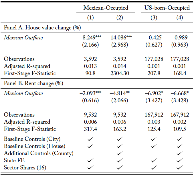
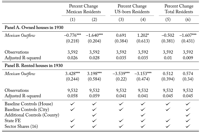
In studying the effects on individual house values and rents, we break down the sample into different types of houses. We define a Mexican-occupied house as an address with 50% or more of their residents in 1930 of Mexican origin. We define a US-born-occupied house as an address where all residents were US-born and not of Mexican descent. Table 3 presents the estimates of the effect of repatriation on the percent changes in house values or rents for Mexican-occupied and US-born-occupied houses. The table presents the estimates of the effect for Mexican-occupied houses (columns 1 and 2), US-born occupied houses (columns 3 and 4). We show the estimates using the percent change in the house value (Panel A) and percentage change in the rent (Panel B). In all regressions, we restrict the sample to the states with more than 0.25% Mexican population share (Arizona, Texas, California, New Mexico, Kansas, Colorado, Wyoming, Utah, Idaho, Nebraska, Indiana).

The results show that the Mexican repatriation had a large and persistent effect on houses where Mexicans lived in 1930. We find that houses inhabited by Mexicans in 1930 devalued 8.2 percentage points between 1930 and 1940 for every percentage point drop in the city’s Mexican population. Houses rented by Mexicans in 1930 also faced decreased rental rates of over 2 percentage points for every percentage point of Mexican outflow.

To illustrate the economic significance of this effect, we can compare it to the median devaluation of Mexican occupied houses in the period. The value of the median house owned by Mexicans fell by 41% between 1930 and 1940. This means that the partial negative effect of the repatriation on Mexican-owned houses is equivalent to one fifth (8.2/41 = 20%) of the decline observed in the median Mexican-occupied house value distribution in our sample. The value of the median rent paid by Mexicans fell by 33% between 1930 and 1940. For rented units, the partial effect of the repatriation is equivalent to six percent (2/33 = 6%) of the decline observed in the median rent of Mexican-occupied houses in our sample. Interestingly, we do not find a statistically significant coefficient on US-born occupied houses’ price change (rents or values).

Table 3. Effects on house-level prices.

This table presents our baseline estimates of the effect of the Mexican repatriation on house values and rents. We estimate the house-level regressions from Equation (4)

$\underset{{1930:40}}{\Delta} Y_{h} = \alpha + \gamma \cdot \Tilde{O}^{MEX}_{1930:40,c} \left( IV_{cty} \right) + \lambda_s + \mathbf{X}_{c, 1930} + \mathbf{X}_{h, 1930} + \epsilon_{h}$

where $\Delta_{1930:40} Y_{h}$ is a house’s 1930–1940 percentage change in its $\textit{House Value}$ or $\textit{Rent}$ . $\Tilde{O}^{MEX}_{1930:40,c} \left( IV_{c} \right)$ is the Mexican outflow between 1930 and 1940 in the city c where the house is located instrumented by $IV_{c}$ , as defined in Equation 3; $\lambda_s$ represents state fixed effects; and $\mathbf{X}_{c,1930}$ is the set of 1930 city-level baseline controls, which include the $\textit{Average Age}$ , average $\textit{School Attendance}$ the share of $\textit{Unemployed}$ workers, and employment $\textit{Sector Shares}$ ; and $\mathbf{X}_{h,1930}$ is the set of 1930 house-level controls that include the $\textit{Average Age of Residents}$ , the $\textit{Dwelling Size}$ and the house level or rent reported in 1930. We define a Mexican-occupied house as an address that had 50% or more of their residents in 1930 of Mexican origin. US-born-occupied houses are addresses that had only US-born and no Mexican descendent residents in 1930. The table presents the estimates of the effect for Mexican-occupied houses (columns 1 and 2) and US-born-occupied houses (columns 3 and 4). In Panel A, we restrict the sample to the houses that were owned in 1930. In Panel B, we restrict to houses that were rented in 1930. All regressions restrict the sample to states with more than 0.25% Mexican population living in urban areas (Arizona, Texas, California, New Mexico, Kansas, Colorado, Wyoming, Utah, Idaho, Nebraska, Indiana). Standard errors in parentheses are clustered by state. Statistical significance: ***p < 0.01, ** p < 0.05, * p < 0.10.

Impacts on Resident Composition

We find that the Mexican repatriation primarily affected Mexican-occupied house prices (values and rents). One natural question is whether this translated into a change in the types of residents in houses inhabited by Mexicans in 1930. We take advantage of the matched address sample and estimate the impact of the Mexican repatriation on the change of resident composition of Mexican-occupied houses. We estimate the following house level specification using two-stage least squares (2SLS) regression analysis:

(5) $\begin{equation*} \underset{{1930:40}}{\Delta} RC_{h} = \alpha + \gamma \cdot \Tilde{O}^{MEX}_{1930:40,c} \left( IV_{cty} \right) + \lambda_s + \mathbf{X}_{c, 1930} + \mathbf{X}_{h, 1930} + \epsilon_{h} \end{equation*}$

where $\Delta_{1930:40} RC_{h}$ is one of our variables that measure the 1930–1940 changes in the resident composition in house h. $\Tilde{O}^{MEX}_{1930:40,c} \left( IV_{cty} \right)$ is the Mexican outflow between 1930 and 1940 in the city c where the house is located instrumented by $IV_{cty}$ , which is the instrument defined in Equation 3; $lambda_s$ represents state fixed effects; and $\mathbf{X}_{c,1930}$ is the set of 1930 city-level baseline controls, which include the $\textit{Average Age}$ , average $\textit{School Attendance}$ , share of $\textit{Unemployed} workers$ , and employment $\textit{Sector Shares}$ ; and $\mathbf{X}_{h,1930}$ is the set of 1930 house level controls that include the $\textit{Average Age of Residents}$ , the $\textit{Number of Residents}$ . The specifications are unweighted, and standard errors are clustered by state. Table 4 presents the results. Using the two-stage least squares (2SLS) approach, we estimate the effect of the Mexican repatriation on the percent change in the house’s 1930–1940 resident composition: Mexican residents (columns 1–2); US-born residents (columns 3–4); and total residents (columns 5–6). In Panel A, we restrict the sample to the houses that were owned by Mexicans in 1930. In Panel B, we restrict it to houses that were rented by Mexicans in 1930.

We find that the Mexican repatriation decreased the number of Mexican residents in Mexican-occupied houses that were owned in 1930. We do not find a robust inflow of US-born residents into those houses in the subsequent decade. When looking at rented housing, the patterns are different. We find an increase in the number of Mexican residents and a decrease in the number of US-born residents. These results show that the houses previously rented by Mexican residents became increasingly less mixed with US-born residents, suggesting increased housing segregation during the period.

Table 4. Effects on house-level resident composition.

This table presents our house-level regressions from estimating Equation (5):

$\underset{{1930:40}}{\Delta} RC_{h} = \alpha + \gamma \cdot \Tilde{O}^{MEX}_{1930:40,c} \left( IV_{cty} \right) + \lambda_s + \mathbf{X}_{c, 1930} + \mathbf{X}_{h, 1930} + \epsilon_{h},$

where $\Delta_{1930:40} RC_{h}$ is the percent change in the house’s 1930–1940 resident composition: Mexican residents (columns 1–2); US-born residents (columns 3–4); and total residents (columns 5–6). $\Tilde{O}^{MEX}_{1930:40,c} \left( IV_{cty} \right)$ is the Mexican outflow between 1930 and 1940 in the city c where the house is located instrumented by $IV_{cty}$ , as defined in Equation 3; $\lambda_s$ represents state fixed effects; and $\mathbf{X}_{c,1930}$ is the set of 1930 city-level baseline controls, which include the $\textit{Average Age}$ , average $\textit{School Attendance}$ , share of $\textit{Unemployed}$ workers, and employment $\textit{Sector Shares}$ ; and $\mathbf{X}_{h,1930}$ is the set of 1930 house-level controls that include the $\textit{Average Age of Residents}$ , the $\textit{Dwelling Size}$ and the house level or rent reported in 1930. Columns 2, 4, and 6 include the additional county-level controls. In Panel A, we restrict the sample to the houses that were owned by Mexicans in 1930. In Panel B, we restrict it to houses that were rented by Mexicans in 1930. All regressions are restricted to states with more than 0.25% Mexican population share (Arizona, Texas, California, New Mexico, Kansas, Colorado, Wyoming, Utah, Idaho, Nebraska, Indiana). Standard errors in parentheses are clustered by state. Statistical significance: *** p < 0.01, ** p < 0.05, * p < 0.10.

Effects of the Repatriation at the City-Level

In the previous section, we show that the Mexican repatriation had larger effects in areas with Mexicans, more particularly in houses of Mexicans. A natural question follows: To what extent the Mexican repatriation mattered to city-level housing growth?

In this section, we study the effects of repatriation to the aggregate housing market. With the instrument available, we estimate the following baseline specification using two-stage least squares (2SLS) regression analysis:

(6) $\begin{equation*} \underset{{1930:40}}{\Delta} Y_{c} = \alpha + \gamma \cdot \Tilde{O}^{MEX}_{1930:40,c} \left( IV_{cty} \right) + \lambda_s + \mathbf{X}_{c, 1930} + \epsilon_{c} \end{equation*}$

where $\Delta_{1930:40} Y_{c}$ is a city’s 1930–1940 growth rate in percentage terms of the housing market outcomes: median reported $\textit{House Value}$ ; $\textit{Rents}$ ; $\textit{Number of Building Permits}$ ; and $\textit{Value of Building Permits}$ ; $\Tilde{O}^{MEX}_{1930:40,c} \left( IV_{cty} \right)$ is the Mexican outflow between 1930 and 1940 in city c instrumented by $IV_{cty}$ which is the instrument defined in Equations 3; $\lambda_s$ represents state fixed effects to capture state-specific, unobservable heterogeneity (e.g., differences in the intensity of the Great Depression between states); and $\mathbf{X}_{c,1930}$ is a set of 1930 city-level controls, which include the $\textit{Average Age}$ , average $\textit{School Attendance}$ , share of $\textit{Unemployed}$ workers, and employment $\textit{Sector Shares}$ . We refer to this set of control variables as baseline controls. $\textit{Average Age}$ and $\textit{School Attendance}$ are important to control for the characteristics of the working-age population in each city. The share of $\textit{Unemployed}$ workers and $\textit{Sector Shares}$ aim to capture the effects of the Depression on housing market outcomes across cities within each state. The unemployment share captures the economic conditions of cities in 1930, while sector shares account for heterogeneous effects of the Depression associated with the sector composition of cities. All regressions are weighted by the city’s working-age population in 1930,²⁵ and standard errors are clustered by state.

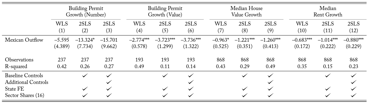
Table 5 presents the estimates of the effect of repatriation on the growth rate of the number of building permits (columns 1–3); the effect on the growth rate of the value of building permits (columns 4–6); the effect on the growth rate of cities’ median house value (columns 7–9); and the effect on the growth rate of cities’ median rent (columns 10–12). Within each real estate outcome in Table 5, the first-ordered columns (columns 1, 4, 7, and 10) show the weighted least squares (WLS) estimates. The second-ordered columns (columns 2, 5, 8, and 11) present 2SLS results using only the baseline controls. The third-ordered columns (columns 3, 6, 9, and 12) present the 2SLS results with the inclusion of the additional controls.

Table 5. Effects on city-level housing, 1930–1940.

This table presents our baseline regressions from estimating Equation (6):

$\underset{{1930:40}}{\Delta} Y_{c} = \alpha + \beta \cdot \Tilde{O}^{MEX}_{1930:40,c} \left( IV_{cty} \right) + \lambda_s + \mathbf{X}_{c, 1930} + \epsilon_{c}$

where $\Delta_{1930:40} Y_{c}$ is a city’s 1930–40 growth rate in one of its housing market outcomes: $\textit{Number of Building Permits}$ ; $\textit{Value of Building Permits}$ ; median reported $\textit{House Value}$ ; and median reported $\textit{Rent}$ ; $\Tilde{O}^{MEX}_{1930:40,c} \left( IV_{cty} \right)$ is the Mexican outflow between 1930 and 1940 in city c instrumented by $IV_{cty}$ , which is the instrument defined in Equation 3; $\lambda_s$ represents state fixed effects to capture state-specific, unobserved heterogeneity; and $\mathbf{X}_{c,1930}$ is a set of 1930 city-level controls, which include the population $\textit{Average Age}$ , average $\textit{School Attendance}$ , share of $\textit{Unemployed}$ workers, and employment $\textit{Sector Shares}$ . The table presents the estimates of the effect of repatriation on the growth rates of the number of building permits (columns 1–3), the building permits value (columns 4–6), the cities median house value (columns 7–9), and cities median rent (columns 10–12). Columns 1, 4, 7, and 10 show $\textit{weighted least squares}$ estimates of Equation 6 without any instrumental variable or control. Columns 2, 5, 8, and 11 present the 2SLS results with $IV_{cty}$ as an instrument for the $\textit{Mexican Outflow}$ and using the baseline controls. Columns 3, 6, 9, and 12 present the 2SLS results with the inclusion of the additional controls: (i) county level characteristics on the retail sales growth (a measure for the Great Depression intensity) from Fishback, Horrace and Kantor (2005); (ii) the intensity of the Dust Bowl environmental catastrophe using county-level measures for months of drought times the county’s farm share from Fishback, Horrace and Kantor (2005), and the fraction of land exposed to medium and high permanent soil erosion during the 1930s from Hornbeck (2012). All regressions are weighted by total working-age population in 1930. Standard errors in parentheses are clustered by state. Statistical significance: *** p < 0.01, ** p < 0.05, * p < 0.10.

The results reveal a negative and statistically significant relationship between the Mexican outflow and all the housing market outcomes. Specifically, a one standard deviation increase in exposure to the Mexican outflow (1 percentage point) leads to a 1.2 percentage points decrease in the average growth rate of the median house value and a one percentage point decrease in the median rent growth rate between 1930 and 1940. These are relatively large compared to the baseline growth rates of these variables in the period. On average, median house values decreased 43.2% while median rents decreased 30.6% in the period. In other words, a one standard deviation increase in exposure to the Mexican repatriation explains approximately 2.8% of the decrease in house values and 3.3% of rents.

We also find that the repatriation negatively affected the growth rate of forward-looking measures based on building permits. An increase of one standard deviation in the exposure to the Mexican outflow (1 percentage point) decreased the average growth rates of our leading indicator variables, the value of permits (–3.7 percentage points), and the number of building permits (–13 percentage points). To put these results in perspective, we can compare these values to the observed average growth rates in these indicators during 1930–40. The partial effect of one standard deviation increase in exposure to the Mexican outflow represents approximately 7.4%, and 8.7% of the building permit growth rates in terms of number and value, respectively. All results are robust to the inclusion of the additional control variables, except the effect on the number of building permits, which loses statistical significance. In the next section, we explore the geographical heterogeneity in the exposure to the Mexican repatriation to further illustrate the implications of our city-level results.

Quantifying the Effect of the Mexican Repatriation

In this section, we use a quasi-counterfactual exercise to illustrate the quantitative implications of our findings. This empirical exercise, similar to the one used by Burchardi, Chaney and Hassan (2018), is not meant to serve as a formal counterfactual, but rather to offer a different perspective to visualize the effects of the Mexican repatriation on housing market outcomes. In this quasi-counterfactual, we ask the question: How different would the growth rates of the housing market in US cities have been had the Mexican repatriation not happened?
To answer this question, we first assume that the general equilibrium effects from the repatriation are either negligible or non-existent. In this case, our reduced-form results could be used to estimate the predicted changes in the outcome variables under the scenario without the Mexican repatriation. We also require an estimate of the outflow of Mexican immigrants in the absence of the Mexican repatriation. We use the data and the estimated coefficients from the first stage to derive a rough estimate. We start by assuming that the repatriation effect is completely captured by our instrumental variables, conditional on the control variables. The underlying assumption is that, if the repatriation had not happened, we would not have observed any effect of the instrumental variables on the Mexican outflow. The results in Table 8 support this idea.

The results show that the instrumental variables are relevant to explaining Mexican immigrants’ outflow and that they do not have a statistically significant association with the outflow of immigrants from other nationalities. We use the estimates from Table 6 of the first stage regressions to obtain the hypothetical Mexican outflow in the absence of the repatriation. We calculate the hypothetical Mexican outflow in the case of no repatriation as $\Ddot{O}^{MEX}_{1930:40,c} \equiv O^{MEX}_{1930:40,c} - \hat{\xi} \cdot IV_{cty}$ , where $O^{MEX}_{1930:40,c}$ is the observed Mexican outflow and $\hat{\xi}$ is the estimated coefficient of the instrumental variable $IV_{cty}$ in the first stage, i.e., Equation 7. We rearrange this expression to represent the predicted change in Mexican outflow as $\mathit{d} O^{MEX}_{1930:40,c} \equiv \hat{\xi} \cdot IV_{cty}$ .

Figure 5. Real estate outcomes without the Mexican repatriation.

(A) Number of Building Permits

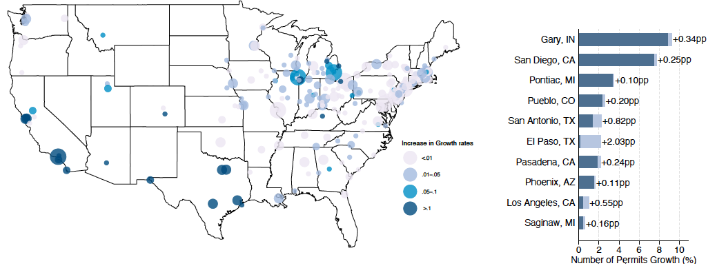
(B) Value of Building Permits

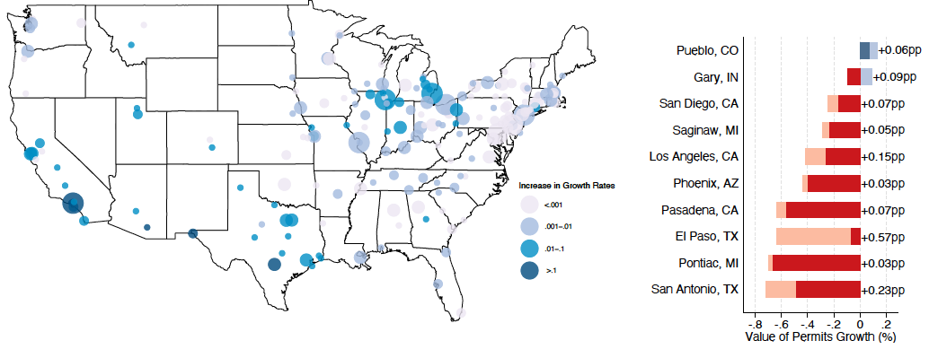
(C) House Value

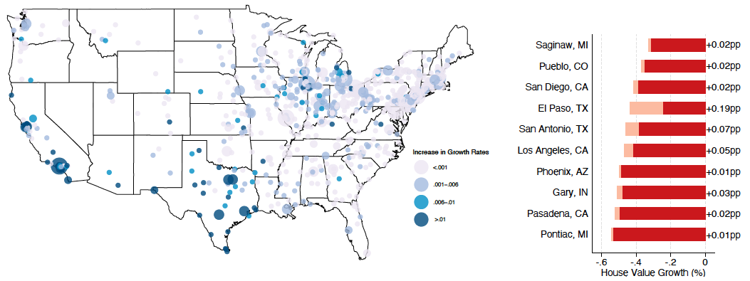
(D) Rents

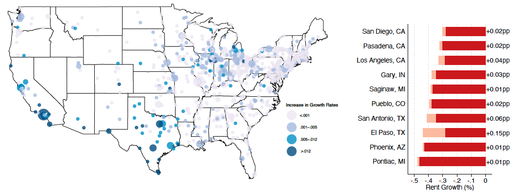
This figure summarizes the quasi-counterfactual for the housing market outcomes of interest: number of building permits (Panel A), value of building permits (Panel B), house value (Panel C), and rents (Panel D). The maps depict the predicted increase in the growth rates of the city’s respective real estate outcome as detailed in Section 4.3. The size of each bubble is proportional to the city’s working age population in 1930. Darker shades of blue represent greater predicted increases in percentage points. The bar graphs show the top 10 cities with highest Mexican outflow between 1930 and 1940 with non-missing information on all outcome variables. For cities with negative growth rates (red bars), the counterfactual (depicted in light red) cancels out the observed decline (depicted in dark red). For cities with positive growth rates (blue bars), the counterfactual (in light blue) increments the observed growth rate (in dark blue).

Given this predicted change in the Mexican outflow, we use the estimates from Table 5 to calculate the hypothetical change in the growth rates of our housing market outcome variables. The predicted change in the outcomes is specified by $\mathit{d} \left[ \underset{{1930:40}}{\Delta} Y_{c} \right] \equiv \hat{\gamma} \cdot \mathit{d} O^{MEX}_{1930:40,c}$ . FIgure 5 illustrates the predicted changes in the growth rates. The maps on the left depict the geographic distribution of the changes, while the bar graphs on the right show the predicted changes for the cities with the highest Mexican outflow between 1930 and 1940. For cities with negative growth rates, the counterfactual (depicted in light red) cancels out the observed decline (depicted in vivid red). For cities with positive growth rates, the counterfactual (in light blue) increments the observed growth rate (in vivid blue).²⁶

The results in Figure 5 suggest that the predicted change in the Mexican outflow would have been highly heterogeneous across US cities, translating into heterogeneous changes in the growth rates of housing market outcomes. We find that the growth rates of the number and value of building permits, house values, and rents would have been significantly larger in the hypothetical scenario of no repatriation, especially for the cities closer to the US–Mexico border. For example, the growth in the number of building permits (Panel A) in El Paso would have been 2.03 p.p. higher in the counterfactual scenario, instead of stagnating around zero. Notably, the striking fall observed in El Paso’s growth rate in the value of building permits (Panel B) would have been almost fully canceled out in the counterfactual. Finally, the deep dive in the actual growth rate of El Paso’s median house value (Panel C) would be roughly cut in half in the counterfactual.

Identification Validity and Robustness

Instrument Validity

In this section, we present standard tests to validate our constructed instrument. Table 6 presents the results of estimating the following first stage regressions:

(7) $\begin{equation*} O^{MEX}_{1930:40,c} = \alpha + \xi \cdot IV_{cty} + \epsilon_{c}. \end{equation*}$

Columns 1–3 present the first stage estimates in the house-level sample, and columns 4–6 show them at the city-level. In columns 1 and 4, we estimate Equation (7) with no controls, fixed effects, and unweighted by city population. Columns 2 and 5 add our baseline controls, state level fixed effects, sector shares, and city population weights to the previous specifications. Columns 3 and 6 include the additional set of controls. The results show that the F-statistics are large and significant in all specifications, alleviating concerns that the instrument is weak.

Table 6. Instrument validation: first stage regressions.

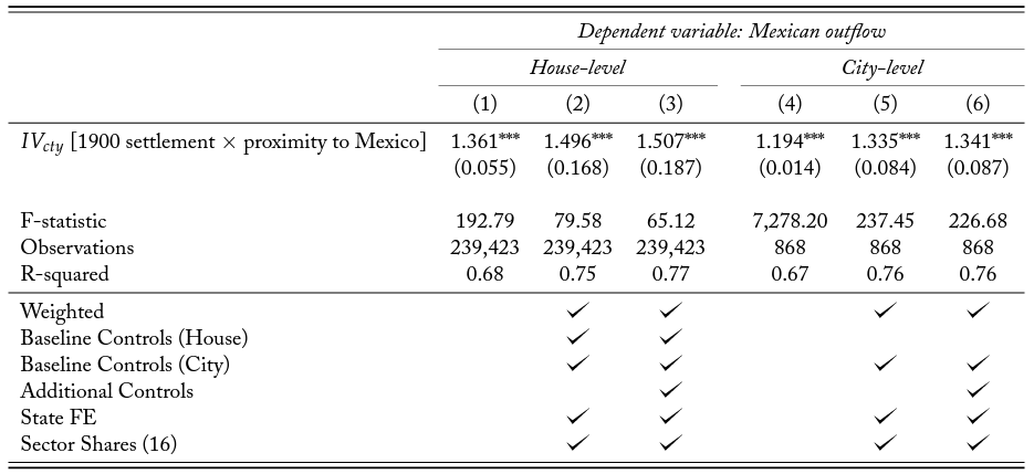
This table presents results for the first-stage regressions of the instrumental variable approach and is one of the IV validation tests that we discuss in Section 5.1. The first-stage regressions are given by Equation 7:

(8) $\begin{equation*} O^{MEX}_{1930:40,c} = \alpha + \xi \cdot IV_{cty} + \epsilon_{c}, \end{equation*}$

where $O^{MEX}_{1930:40,c}$ is the Mexican outflow between 1930 and 1940 in any given city c. $IV_{cty}$ combines the proximity to the Mexican border interacted with the share of Mexican immigrants in 1900. Columns 1–3 show the first stage regression at the address level sample, while columns 4–6 show the estimates at the city level. In Columns 1 and 4, we estimate Equation 7. Columns 2 and 5 add city-level controls (1930 Census city-level $\textit{Average Age}$ , $\textit{School Attendance}$ , and share of $\textit{Unemployed}$ workers), state fixed effects, sector employment shares, and city population weights (i.e., weighted least squares estimation) to the previous specifications. Columns 3 and 6 include the additional controls: (i) the interaction of the number of severe drought months faced by a county and the county’s share of farming land; (ii) the retail sales growth rate between 1929 and 1935; (iv) the log of the city-level median house value in 1930; (v) the fraction of each county exposed to medium and high permanent soil erosion due to the American Dust Bowl in the 1930s. Controls are described in more detail in Table 2. The table also includes the Kleibergen-Paap $F$ -statistics on the excluded instrument for each of the IV specifications to test for weak identification. Standard errors are clustered by state for all specifications. Statistical significance: *** p < 0.01, ** p < 0.05, * p < 0.10.

Another concern regarding our instrumental variable approach is whether our IV satisfies the exclusion restriction. Our instrumental variable approach requires that the Mexican settlements in 1900 interacted with the proximity to the US-Mexico border are not correlated with unobserved factors that determined the housing market changes in 1930–1940, after controlling for demographic and economic local characteristics, state fixed effect and sector employment share. One potential concern is that the IV is mechanically correlated with the intensity of the Great Depression. Our motivation to use the IV approach is precisely that it mitigates this mechanical relationship with the economic impact of the Great Depression.

We run a series of tests to analyze the partial correlation between our IV and the intensity of the Great Depression in each city. We begin by using census data on each city’s change in total unemployment between 1930 and 1940, normalized by the total working-age population as a measure of the economic conditions from the Great Depression. We then use the change in unemployment in the agricultural, and non-agricultural sectors as two complementary measures for different dimensions of the intensity of the Great Depression. In addition to the unemployment-based measures, we rely on the data collected by Fishback, Horrace and Kantor (2005) on the growth rate of retail sales for each US county as an alternative measure. Formally, we estimate:

(9) $\begin{equation*} \Delta GD_{c} = \alpha + \beta \cdot IV_{cty} + \lambda_s + \mathbf{X}_{c, 1930} + \epsilon_{c}, \end{equation*}$

where $\Delta GD_{c}$ is one of the measures of the intensity of the Great Depression in city c: the 1930–1940 change in total unemployment; 1930–1940 change in unemployment in agriculture sectors; 1930–1940 change in unemployment in non-agriculture sectors; and the 1929–1935 growth rate of retail sales in the county where city c is located. Other variables are defined as before. Results are shown in Table 7. The estimates show that our instrument is not significantly correlated with an important measure of consumption. Thus it is not significantly correlated with this measure of aggregate economic activity during the Great Depression.

We also conduct a complementary set of tests using Wallis’s (1989) state-level data from the US Bureau of Labor Statistics (BLS) on non-agricultural employment (split into manufacturing and non-manufacturing sectors) between 1929 and 1939. Appendix Figure B.5 shows the data and the results of the estimations in Table B.4. The results confirm that our instrument is not significantly correlated with the state-level economic conditions of the Great Depression.

In summary, our results in Table 7 and Table B.4 show that none of the estimated correlation coefficients are statistically significant. Therefore, the results suggest that our instrumental variables are not correlated with various measures of the Great Depression, which is consistent with the exclusion restriction requirement for IV validity.

Table 7. Instrument validation: Mexican outflow and IV correlation with Great Depression intensity measures.

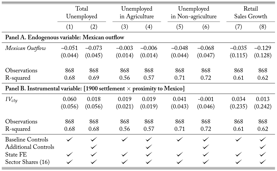
This table is one of the IV validation tests we describe in Section 5.1. The construction of our IV is described in Section 3.1. Regressions are at the city level and weighted by cities’ working-age population in 1930. The dependent variables are measured in percentage change. This set of results uses census information on the city’s change in total number of unemployed workers and unemployed workers in agriculture and non-agriculture between 1930 and 1940 and the change in retail sales between 1929 and 1935. We estimate the following specification:

$\underset{{1930:40}}{\Delta} GD_{c} = \alpha + \beta \cdot IV_{cty} + \lambda_s + \mathbf{X}_{c, 1930} + \epsilon_{c},$

where $\underset{{1930:40}}{\Delta} GD_{c}$ is one of the measures of the adverse economic conditions accrued from the Great Depression: the change in the number of unemployed workers, unemployed workers in agriculture sectors, unemployed workers in non-agriculture sectors, and retail sales growth. The first three measures are calculated using census information on the city’s change in the unemployed population between 1930 and 1940, normalized by the total working-age population in 1930. The retail sales-based measure is the growth rate in retail sales between 1929 and 1935 in each county from Fishback, Horrace, Kantor (2005). All specifications include the baseline controls (1930 Census city-level $\textit{Average Age}$ , $\textit{School Attendance}$ , and share of $\textit{Unemployed}$ workers), state fixed effects, and sector employment shares. Columns 2, 4, and 6 include the additional controls (the number of severe drought months interacted with the share of farming land, the retail sales growth rate between 1929 and 1935, the log of the city-level median house value in 1930, the fraction of each county exposed to medium and high permanent soil erosion due to the American Dust Bowl in the 1930s). Column 8 includes all the previous variables, except retails sales growth, which is the dependent variable in that specification. Standard errors are clustered by state for all specifications. Statistical significance: *** p < 0.01, ** p < 0.05, * p < 0.10.

Finally, we examine whether our constructed instrumental variables capture variation in the 1930–1940 outflow of migrants from other countries. If we reject the null hypothesis that the instrument is not linearly associated with the outflow of immigrants of other nationalities, then this could raise concerns about the validity of the exclusion restrictions. For this test, we choose three groups of immigrants: (i) Latin Americans (other than Mexicans) because of their cultural and occupational similarity to the Mexican immigrants; (ii) Canadians because of the geographic similarity to Mexico in terms of being a neighbor country to the US; (iii) Asians because immigrants from Asia, especially of Chinese origin, were the first group of immigrants to be targeted by immigration policies that aimed to limit entry based on race or country of origin.²⁷ Table 8 presents the result of estimating a first-stage regression specification, but using the outflow of different nationalities as the dependent variable instead of the outflow of Mexicans:

(10) $\begin{equation*} O^{n}_{1930:40,c} = \alpha + \beta \cdot IV_{cty} + \mathbf{X}_{c, 1930} + \epsilon_{c}, \end{equation*}$

where $O^{n}_{1930:40,c}$ represents the 1930–40 population outflow of nationality $n$ —which can be $\textit{Mexican}$ , $\textit{Latin American (other than Mexican)}$ , $\textit{Canadian}$ , or $\textit{Asian}$ —in each city. In Columns 1, 3, 5, and 7, we estimate Equation 7 for $IV_{cty}$ , including the baseline city-level controls (1930 Census city-level averages of $\textit{Population Age}$ , $\textit{School Attendance}$ , and share of $\textit{Unemployed}$ workers), state fixed effects, sector shares, and city population weights (i.e., weighted least squares estimation) to the previous specifications. Columns 2, 4, 6, and 8 include the additional controls by Fishback, Horrace, and Kantor (2005): (i) the interaction on the number of severe drought months faced by a county and the county’s share of farming land; (ii) the retail sales growth rate between 1929 and 1935; and (iii) the log of the city-level median house value in 1930, and Dust Bowl controls from Hornbeck (2012): (iv) the fraction of each county exposed to $\textit{Medium}$ and $\textit{High}$ permanent soil erosion due to the American Dust Bowl in the 1930s. None of the validation tests show a statistically significant coefficient between our instrument and various measures of the Great Depression’s intensity or the outflow of immigrants from other nationalities.

Table 8. Instrument validation: instrumental variable and correlation with outflow from other nationalities.

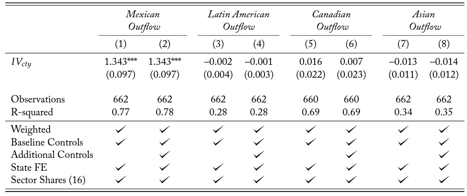
This table is one of the IV validation tests we describe in Section 5.1. It presents the results for the regression of the outflow of immigrants from other nationalities $O^{n}_{1930:40,c}$ on our instrumental variable. The construction of the IV is described in Section 3.1. Specifically, the regressions are:

$O^{n}_{1930:40,c} = \alpha + \beta \cdot IV_{cty} + \mathbf{X}_{c, 1930} + \epsilon_{c}.$

In Columns 1, 3, 5, and 7, we estimate Equation 9 for $IV_{cty}$ , adding the baseline city-level controls (1930 Census city-level $\textit{Average Age}$ , $\textit{School Attendance}$ , and share of $\textit{Unemployed} workers)$ . Columns 2, 4, 6, and 8 include the additional controls: $\textit{Drought Exposure}$ , which is the interaction on the number of severe drought months faced by a county and the county’s share of farming land; the $\textit{Retail Sales Growth}$ rate between 1929 and 1935; the log of the city-level median house value in 1930; the fraction of each county exposed to $\textit{Medium}$ and $\textit{High}$ permanent soil erosion due to the American Dust Bowl in the 1930s. All specifications include state fixed effects, sector employment shares from 1930, and city population weights. In all regressions, we exclude from the sample the cities with net inflow of Mexicans. Standard errors in parentheses are clustered by state. Statistical significance: *** p < 0.01, ** p < 0.05, * p < 0.10.

House Market Effects: Robustness to Different Percentiles of Values and Rents

Taking advantage of the full-count census data available, we expand the analysis to investigate the sensitivity of the impact of Mexican repatriation across the distribution of house values and rents.²⁸ We examine the effects across different percentiles within cities by estimating the repatriation effect at different percentiles of the house value and rent distributions. The equation we estimate is analogue to Equation (6) and is given by:

(11) $\begin{equation*} \underset{{1930:40}}{\Delta} Y_{c}(\tau) = \alpha + \beta \cdot \Tilde{O}^{MEX}_{1930:40,c} \left( IV_{cty} \right) + \lambda_s + \mathbf{X}_{c, 1930} + \epsilon_{c}, \end{equation*}$

where $\Delta_{1930:40} Y_{c}(\tau)$ is a city’s 1930–40 growth rate in reported $\textit{House Value}$ or $\textit{Rent}$ at percentile $\tau$ . We obtain, for each city, the house value or rent at several points of the house value or rent distribution. Specifically, to avoid the influence of outliers, we consider the interquartile range range (i.e., from the 25th to the 75th percentile), breaking it down into 10 percent intervals. The estimated coefficients and 95% confidence intervals of the two-stage least squares (2SLS) estimates are presented in Figure 6. The median (50th percentile) effect—already shown in Table 5—is highlighted in the figures.

Figure 6. Heterogeneous effects at different percentiles of the within-city house value and rent distribution.

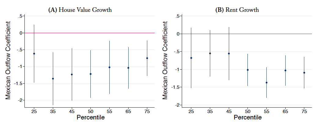
This figure reestimates the House Value Growth and the Rent Growth equations from our baseline specification in Columns 9 and 12 of Table 5 but uses the growth rates at different percentiles of each city’s House Value and Rent distributions as the dependent variable. The figure shows the coefficients and 95% confidence intervals for the two-stage least squares (2SLS) estimates of the Mexican outflow on house value growth (Panel A) and rent growth (Panel B). All specifications include the baseline control variables, sector employment shares, and state fixed effects.

Event Study Specification

One concern with our identification strategy is the possibility that the share of Mexican workers in 1930 is associated with socioeconomic changes that occurred in the previous years that could also be associated with the housing market outcomes.

The presence of “pre-trends” would be taken as evidence against our identification assumption. To take this into account, we estimate an additional set of event-study specifications for the 1921–1940 period:

(12) $\begin{equation*} \underset{{t-1:t}}{\Delta} Y_{c} = \alpha + \beta_{t} \cdot \left( \frac{Pop^{MEX}_{c,1930} }{Pop_{c,1930}} \right) + \lambda_s + \epsilon_{c}, \end{equation*}$

where $\Delta_{t-1:t} Y_{c}$ is a city’s annual growth rate in either the number or the value of building permits; $\nicefrac{Pop^{MEX}_{c,1930} }{Pop_{c,1930}}$ is a city’s share of Mexican workers in 1930; $\lambda_s$ represents state fixed effects, and t are the available years.²⁹ We cannot estimate a similar specification for the median house value or median rent because this information was not collected before the 1930 Census.

Figure 7 shows the estimated coefficients $\beta_t$ with 95% confidence intervals. In addition to showing how the Mexican repatriation effect evolves, the coefficients for years before 1929 provide a direct test for pre-existing effects, supporting our identification strategy. The figures also shed light on the dynamics of the effect of the repatriation on the number and value of permits. For instance, the negative effect on the number of permits is immediately evident in 1930, while the effects on the value of permits is significant only one year after in 1931. Another interesting result is that the negative effects are concentrated over the years when the repatriation was more intense (1930–1934). It is also interesting that in 1935 growth rates for the number of permits were positively associated with the share of Mexicans. This same effect emerged one year later, in 1936, for the value of building permits.³⁰ Despite this short-term recovery, the overall effect of the repatriation along the decade remains negative, as shown in Table 5.

Sensitivity to the Exclusion of Cities not Directly Exposed

One of the concerns with our baseline analysis is that our sample includes many cities that were not directly exposed to the Mexican repatriation. In this section, we investigate the sensitivity of our baseline estimates to different strategies to account for these non-affected cities. We re-estimate our baseline specifications, performing various sample restrictions to exclude the cities that were not directly affected to the Mexican repatriation. We also estimate the baseline regression but weighting for the total number of Mexican workers instead of total working-age population. The goal is to study the sensitivity of the coefficients to imposing heavier weights on cities that had more Mexican workers in 1930.

Figure 7. Share of Mexicans in 1930 and annual building permit growth, 1921–1940.

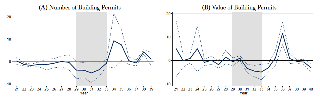
This figure shows coefficients of the share of Mexican workers in 1930 using the event study specification on the annual growth rate of the number of building permits (Panel A) and the growth rate of the value of building permits (Panel B). The lines are the point estimates from the event study specification with 95% confidence intervals. The shaded areas represent the Great Depression period dated by the NBER. Standard errors are clustered by state.

Table 9 presents the estimated coefficients for Number of Building Permits (Column 1); Value of Building Permits (Column 2); median House Value (Column 3); and median Rent (Column 4); estimated by two-stage least squares (2SLS) using our IV, which is defined in Equation (3). All specifications include the baseline controls, sector employment shares, and state fixed effects. In Panel A, we exclude from the sample the cities with fewer than five Mexican workers in 1930.³¹ In Panel B, we restrict the sample to the states that had more than 0.25% of their working age population composed by Mexican workers in 1930 (Arizona, Texas, California, New Mexico, Kansas, Colorado, Wyoming, Utah, Idaho, Nebraska, and Indiana). In Panel C, we restrict the sample to the states that contained the top 25 cities with the largest Mexican outflow rates (Texas, California, Indiana, Arizona, Colorado, Ohio, and New Mexico). All regressions are weighted by the total working-age population in 1930. In Panels B and C, we do not include the sector employment shares as controls due to the small sample sizes.

Table 9. Robustness to the exclusion of cities with few or no Mexican workers in 1930: effects on housing market, 1930–40.

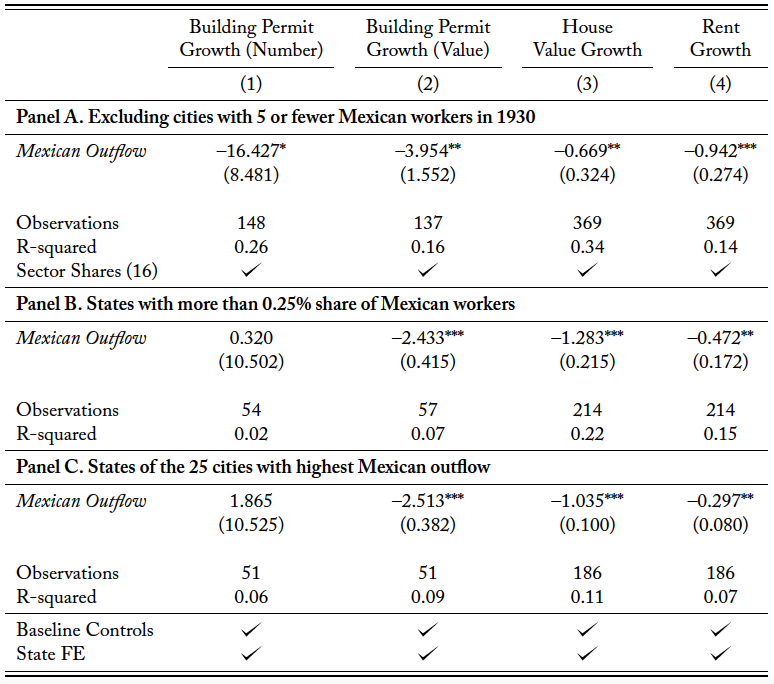
This table presents the estimates of the baseline regressions, but performing various sample restrictions to account for the cities that were not exposed to the Mexican repatriation. The goal is to study the sensitivity of our estimates to the exclusion of the cities not directly affected by the Mexican repatriation. The regressions are estimated as given by Equation (6):

$\underset{{1930:40}}{\Delta} Y_{c} = \alpha + \beta \cdot \Tilde{O}^{MEX}_{1930:40,c} \left( IV_{cty} \right) + \lambda_s + \mathbf{X}_{c, 1930} + \epsilon_{c},$

where $\Delta_{1930:40} Y_{c}$ is a city’s 1930–40 growth rate in one of its housing market outcomes: $\textit{Number of Building Permits}$ (Column 1); $\textit{Value of Building Permits}$ (Column 2); median reported $\textit{House Value}$ (Column 3); and median reported $\textit{Rent} (Column 4); \(\Tilde{O}^{MEX}_{1930:40,c} \left( IV_{cty} \right)$ is the Mexican outflow between 1930 and 1940 in city c instrumented by $IV_{cty}$ , which is defined in Equation 3; $\lambda_s$ represents state fixed effects to capture state-specific, unobserved heterogeneity; and $\mathbf{X}_{c,1930}$ is the set of city-level controls, which include the population $\textit{Average Age}$ , average $\textit{School Attendance}$ , share of $\textit{Unemployed}$ workers, and employment $\textit{Sector Shares}$ . In Panel A, we exclude from the sample the cities with fewer than 5 Mexican workers in 1930. In Panel B, we restrict the sample to the states that had more than 0.25% of their working age population composed by Mexican workers in 1930 (Arizona, Texas, California, New Mexico, Kansas, Colorado, Wyoming, Utah, Idaho, Nebraska, and Indiana). In Panel C, we restrict the sample to the states that contained the top 25 cities with the largest Mexican outflow rates (Texas, California, Indiana, Arizona, Colorado, Ohio, and New Mexico). Standard errors in parentheses are clustered by State. Statistical significance: *** p < 0.01, ** p < 0.05, * p < 0.10.

In summary, the results are qualitatively similar to the baseline results on Table 5, suggesting that the results are robust to different sample restrictions to cities with at least one Mexican immigrant in 1930.

Effects on Supply of Housing: Employment in Construction Industry

In 1930, a significant share of the Mexican immigrant workers was employed in the construction and related manufacturing sectors industries. Table B.3 shows that approximately 12.7% of the Mexican workers were employed in the construction and related sectors. Therefore, the repatriation might have also affected the supply of housing through employment in these sectors.

Table 10 presents estimates of how the repatriation affected changes in employment in the construction industry to Mexicans (columns 1–3), US-born (columns 4–6) and total employment (columns 7–9), all relative to the total working-age population in each city. The first set of results (columns 1–3) is not surprising. It shows a negative effect of the repatriation on the share of employment of Mexicans in the construction sector. The second set of regressions (columns 4–6) shows that cities more affected by repatriation had an increase in the employment of US-born in construction. However, once we consider the total employment in the construction sector (columns 7–9), we find a small and statistically insignificant effect.

Taken together, these results suggest that the repatriation induced the substitution of Mexicans by US-born workers in the construction and construction-related sectors and a stagnation of the overall employment growth in these sectors. This is in line with the employment results spanning all sectors estimated by Lee, Peri and Yasenov (2022).

Table 10. Effects on employment in the construction industries, 1930–1940.

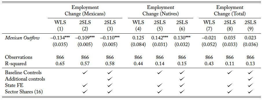
This table presents the results from estimating:

$\underset{{1930:40}}{\Delta} Emp^{Mex|US|Tot}_{c} = \alpha + \beta \cdot \Tilde{O}^{MEX}_{1930:40,c} \left( IV_{cty} \right) + \lambda_s + \mathbf{X}_{c, 1930} + \epsilon_{c},$

where $\Delta_{1930:40} Emp^{Mex|US|Tot}_{c}$ is a city’s employment change in the construction industries between 1930 and 1940 for each group of workers: Mexican ( $\textit{Mex}$ ) employment, US-born ( $\textit{US}$ ), and total ( $\textit{Tot}$ ) employment. $\Tilde{O}^{MEX}_{1930:40,c} \left( IV_{cty} \right)$ is the Mexican outflow between 1930 and 1940 in city c instrumented by $IV_{cty}$ , which is the instrument defined in Equation 3; $\lambda_s$ represents state fixed effects to capture state-specific, unobserved heterogeneity; and $\mathbf{X}_{c,1930}$ is a set of 1930 city-level controls, which include the population $\textit{Average Age}$ , average $\textit{School Attendance}$ , share of $\textit{Unemployed}$ workers, and employment $\textit{Sector Shares}$ . The table presents the estimates of the effect of repatriation on the growth of the employment of Mexicans (columns 1–3), on the growth of the employment of US-born (columns 4–6) and on the growth of total employment (columns 7–9) in the construction industries. Columns 1, 4, and 7 show $\textit{weighted least squares}$ estimates, columns 2, 5, and 8 present the 2SLS results with the inclusion of the baseline controls. Columns 3, 6, and 9 include the additional controls: $\textit{Drought Exposure}$ , which is the interaction on the number of severe drought months faced by a county and the county’s share of farming land; the $\textit{Retail Sales Growth}$ rate between 1929 and 1935; the log of the city-level median house value in 1930; the fraction of each county exposed to $\textit{Medium}$ and $\textit{High}$ permanent soil erosion due to the American Dust Bowl in the 1930s. All regressions are weighted by total working-age population in 1930 and include state fixed effects. Standard errors in parentheses are clustered by state. Statistical significance: *** p < 0.01, ** p < 0.05, * p < 0.10.

Concluding Remarks

In this paper, we evaluate the effects of the United States’ Mexican repatriation of the 1930s on housing markets. Housing is a crucial channel through which migration affects the local economy and wealth distribution. However, most of what we know about the migration effects on housing comes from studies that focus on the inflows of immigrants. This paper is the first to quantify the impact of out-migration on housing empirically. Making this distinction when studying housing markets is indispensable. Because housing is durable, and housing investment is naturally irreversible, asymmetric effects on prices may arise.

This paper studies one of the largest ethnically motivated migration shocks in US history to examine the impact of an out-migration shock on local housing, the United States’ Mexican repatriation of the 1930s. To leverage the rich micro-level data from the census, we develop a novel automated matching technique to link addresses across the 1930 and 1940 Censuses. To isolate the effect of the Mexican repatriation, we employ an instrumental variable approach that combines the historical presence of Mexican immigrants in the US with a measure of the cost of repatriating workers (the proximity to the US-Mexico border based on the US road infrastructure).

We find that the value of houses inhabited by Mexicans in 1930 devalued by an average of 8.2 percentage points between 1930 and 1940 for every percentage point drop in a city’s Mexican population. Rents on houses occupied by Mexicans in 1930 also fell by more than 2 percentage points for every percentage point of Mexican outflow. We find that the repatriation also mattered for the evolution of city-level housing market outcomes. The repatriation decreased the growth rates of coincident indicators (median house value or rents) and incidental indicators (number and value of building permits) of the city-level housing markets.

The renewed political rhetoric against immigration, including a rise in the advocates for repatriations in many developed countries suggest that these types of immigration policies have become a popular option among some voters. What lessons can we learn from the Mexican repatriation of 1930 about how the repatriation policies can influence modern housing markets? Despite some specificities of the period we study, our findings can contribute to the public debate regarding the economic consequences of repatriation policies. We find that implementing a repatriation, especially a large-scale repatriation, would be quite costly to housing growth. Our findings suggests strong negative effects on prices for houses of the affected population, with no clear benefit to the local native residents. At the city-level, the slower growth in these housing-market outcomes suggests that repatriation policies can have impacts on different types of real estate activity, including single-family homes and commercial construction. Therefore, our results serve as a cautionary tale for policymakers in advanced and emerging economies engaged in pursuing repatriation policies. Repatriations are episodes with long-lasting impacts on the cultural and social dimensions, but also leave footprints on economic activity.

References

Abramitzky, Ran and Leah Boustan, “Immigration in American Economic History,” Journal of Economic Literature, 2017, 55 (4), 1311–45.

—, — , Katherine Eriksson, James Feigenbaum, and Santiago Pérez, “Automated Linking of Historical Data,” Journal of Economic Literature, September 2021, 59 (3), 865–918.

, Leah Platt Boustan, and Katherine Eriksson, “Europe’s Tired, Poor, Huddled Masses: Self-Selection and Economic Outcomes in the Age of Mass Migration,” American Economic Review, 2012.

—, — , and — , “A Nation of Immigrants: Assimilation and Economic Outcomes in the Age of Mass Migration,” Journal of Political Economy, 2014, 122 (3), 467–506.

—, Philipp Ager, Leah Platt Boustan, Elior Cohen, and Casper Worm Hansen, “The Effects of Immigration on the Economy: Lessons From the 1920s Border Closure,” NBER Working Paper n.26536, 2020.

Akbar, Prottoy A., Sijie Li, Allison Shertzer, and Randall P. Walsh, “Racial Segregation in Housing Markets and the Erosion of Black Wealth,” Technical Report, National Bureau of Economic Research 2019.

Akbari, Ather H. and Yigit Aydede, “Effects of Immigration on House Prices in Canada,” Applied Economics, 2012, 44 (13), 1645–1658.

Alesina, Alberto, Armando Miano, and Stefanie Stantcheva, “Immigration and Redistribution,” NBER Working Paper n. 24733, 2018.

Alix-Garcia, Jennifer, Anne Bartlett, and David Saah, “Displaced Populations, Humanitarian Assistance and Hosts: A Framework for Analyzing Impacts on Semi-Urban Households,” World Development, 2012, 40 (2), 373–386.

Balderrama, Francisco E. and Raymond Rodríguez, Decade of Betrayal: Mexican Repatriation in the 1930s, The University of New Mexico Press, 2006.

Balkan, Binnur, Elif Tok, Huzeyfe Torun, and Semih Tumen, “Immigration, Housing Rents, and Residential Segregation: Evidence from Syrian Refugees in Turkey,” IZA Working Paper No. 11611, 2018.

Becker, Sascha O. and Andreas Ferrara, “Consequences of Forced Migration: A Survey of Recent Findings,” Labour Economics, 2019.

Bennett, David Harry, Demagogues in the depression: American radicals and the Union Party, 1932-1936, New Brunswick, NJ: Rutgers University Press, 1969.

Boustan, Leah Platt, Matthew E Kahn, Paul W Rhode, and Maria Lucia Yanguas, “The effect of natural disasters on economic activity in US counties: A century of data,” Journal of Urban Economics, 2020, 118, 103257.

Brocker, Michael and Christopher Hanes, “The 1920s American Real Estate Boom and the Downturn of the Great Depression: Evidence from City Cross-Sections,” in Eugene N. White, Kenneth Snowden, and Price Fishback, eds., Housing and Mortgage Markets in Historical Perspective, Chicago, University of Chicago Press, 2014.

Burchardi, Konrad B., Thomas Chaney, and Tarek A. Hassan, “Migrants, Ancestors, and Foreign Investments,” Review of Economic Studies, 2018, 86 (4), 1448–1486.

Chaney, Eric and Richard Hornbeck, “Economic Dynamics in the Malthusian Era: Evidence from the 1609 Spanish Expulsion of the Moriscos,” Economic Journal, 2016, 126 (594), 1404–1440.

Clemens, Michael A., Ethan G. Lewis, and Hannah M. Postel, “Immigration Restrictions as Active Labor Market Policy: Evidence from the Mexican Bracero Exclusion,” American Economic Review, 2018, 108 (6), 1468–87.

Cooke, Timothy W. and Bruce W. Hamilton, “Evolution of Urban Housing Stocks: A Model Applied to Baltimore and Houston,” Journal of Urban Economics, 1984, 16 (3), 317–338.

Cortes, Gustavo S. and Marc D. Weidenmier, “Stock Volatility and the Great Depression,” Review of Financial Studies, 2019, 32 (9), 3544–3570.

Courtemanche, Charles and Kenneth Snowden, “Repairing a mortgage crisis: HOLC lending and its impact on local housing markets,” Journal of Economic History, 2011, 71 (2), 307–337.

Depetris-Chauvin, Emilio and Rafael J. Santos, “Unexpected Guests: The Impact of Internal Displacement Inflows on Rental Prices in Colombian Host Cities,” Journal of Development Economics, 2018, 134, 289–309.

Edo, Anthony, Yvonne Giesing, Jonathan Öztunc, and Panu Poutvaara, “Immigration and electoral support for the far-left and the far-right,” European Economic Review, 2019, 115, 99–143.

Enciso, Fernando Saúl Alanís, They Should Stay There: The Story of Mexican Migration and Repatriation During the Great Depression, UNC Press Books, 2017.

Escamilla-Guerrero, David, “Revisiting Mexican Migration in the Age of Mass Migration: New Evidence from Individual Border Crossings,” Historical Methods: A Journal of Quantitative and Interdisciplinary History, 2020, 53 (4), 207–225.

Feigenbaum, James J., “Automated Census Record Linking: A Machine Learning Approach,” Working Paper, 2016.

Feigenberg, Benjamin, “Fenced Out: The Impact of Border Construction on US-Mexico Migration,” American Economic Journal: Applied Economics, 2020, 12 (3), 106–139.

Ferrara, Andreas and Price V. Fishback, “Discrimination, Migration, and Economic Outcomes: Evidence from World War I,” Technical Report, NBER Working Paper n.26936 2020.

Fishback, Price, “How successful was the new deal? The microeconomic impact of new deal spending and lending policies in the 1930s,” Journal of Economic Literature, 2017, 55 (4), 1435–85.

Fishback, Price V., Alfonso Flores-Lagunes, William C. Horrace, Shawn Kantor, and Jaret Treber, “The influence of the Home Owners’ loan corporation on housing markets during the 1930s,” Review of Financial Studies, 2011, 24 (6), 1782–1813.

—, William C. Horrace, and Shawn Kantor, “Did New Deal Grant Programs Stimulate Local Economies? A Study of Federal Grants and Retail Sales During the Great Depression,” Journal of Economic History, 2005, 65 (3), 36–71.

Gjerstad, Steven D. and Vernon L. Smith, Rethinking Housing Bubbles: The Role of Household and Bank Balance Sheets in Modeling Economic Cycles, Cambridge University Press, 2014.

Glaeser, Edward L. and Joseph Gyourko, “Urban Decline and Durable Housing,” Journal of Political Economy, 2005,113 (2), 345–375.

Goetzmann, William N. and Frank Newman, “Securitization in the 1920’s,” NBER Working paper n.15650, 2010.

Gonzalez, Libertad and Francesc Ortega, “Immigration and Housing Booms: Evidence from Spain,” Journal of Regional Science, 2013, 53 (1), 37–59.

Gratton, Brian and Emily Merchant, “Immigration, Repatriation, and Deportation: The Mexican-Origin Population in the United States, 1920–1950,” International Migration Review, 2013, 47 (4), 944–975.

Greulich, Erica, John M. Quigley, Steven Raphael, Joseph Tracy, and Guillermina Jasso, “The Anatomy of Rent Burdens: Immigration, Growth, and Rental Housing,” Brookings-Wharton Papers on Urban Affairs, 2004,149–205.

Guerin-Gonzales, Camille, Mexican workers and American dreams: Immigration, repatriation, and California farm labor, 1900-1939, Rutgers University Press, 1994.

Hoffman, Abraham, “Mexican Repatriation Statistics: Some Suggested Alternatives to Carey McWilliams,” Western Historical Quarterly, 1972, 3 (4), 391–404.,

—, Unwanted Mexican Americans in the Great Depression: Repatriation Pressures, 1929-1939, University of Arizona Press, 1974.

Hornbeck, Richard, “The Enduring Impact of the American Dust Bowl: Short-and Long-Run Adjustments to Environmental Catastrophe,” American Economic Review, 2012, 102 (4), 1477–1507.

—, “Dust Bowl Migrants: Environmental Refugees and Economic Adaptation,” Working Paper, 2021.

Hornung, Erik, “Immigration and the diffusion of technology: The Huguenot diaspora in Prussia,” American Economic Review, 2014, 104 (1), 84–122.

Howard, Greg, “The Migration Accelerator: Labor Mobility, Housing, and Demand,” American Economic Journal: Macroeconomics, October 2020, 12 (4), 147–79.

Jaeger, David A., Joakim Ruist, and Jan Stuhler, “Shift-share Instruments and the Impact of Immigration,” Technical Report, National Bureau of Economic Research 2018.

Johansen, Leif, “Substitution Versus Fixed Production Coefficients in the Theory of Economic Growth: A Synthesis,” Econometrica, 1959, pp. 157–176.

Johnson, Kevin R., “The Forgotten Repatriation of Persons of Mexican Ancestry and Lessons for the War on Terror,” Pace Law Review, 2005, 26, 1.

Johnson, Noel D. and Mark Koyama, “Jewish Communities and City Growth in Preindustrial Europe,” Journal of Development Economics, 2017, 127, 339–354.

Lee, Erika, At America’s Gates: Chinese Immigration During the Exclusion Era, 1882-1943, Univ of North Carolina Press, 2003.

Lee, Jongkwan, Giovanni Peri, and Vasil Yasenov, “The Labor Market Effects of Mexican Repatriations: Longitudinal Evidence from the 1930s,” Journal of Public Economics, 2022, 205, 104558.

Manson, Steven, Jonathan Schroeder, David Van Riper, Tracy Kugler, and Steven Ruggles, “IPUMS National Historical Geographic Information System: Version 15.0 [dataset]. Minneapolis: University of Minnesota,” 2020.

Mathy, Gabriel and Nicolas L. Ziebarth, “How Much does Political Uncertainty Matter? The Case of Louisiana under Huey Long,” Journal of Economic History, 2017, 77 (1), 90–126.

Morin, Miguel and Scott N. Swisher, “The Effect of Infrastructure Investment in a Low-Growth Environment: Evidence from the Great Depression,” Working Paper, University of Cambridge, 2016.

Mussa, Abeba, Uwaoma George Nwaogu, and Susan Pozo, “Immigration and Housing: A spatial Econometric Analysis,” Journal of Housing Economics, 2017.

Ottaviano, Gianmarco I.P. and Giovanni Peri, “Wages, Rents and Prices: The Effects of Immigration on US Natives,” Center for Research and Analysis of Migration, Discussion Paper, 2006, 13 (07).

Price, Joseph, Kasey Buckles, Jacob Van Leeuwen, and Isaac Riley, “Combining Family History and Machine Learning to Link Historical Records: The Census Tree Data Set,” Explorations in Economic History, 2021.

Romer, Margaret, “A History of Calexico,” Annual Publication of the Historical Society of Southern California, 1922, 12 (2), 26–66.

Ruggles, Steven, Catherine A. Fitch, Ronald Goeken, Josiah Grover, David Hacker, Matt Nelson, Jose Pacas, Evan Roberts, and Matthew Sobek, “IPUMS Restricted Complete Count Data: Version 2.0 [dataset],” Minneapolis, MN: University of Minnesota, 2020.

—, Sarah Flood, Ronald Goeken, Josiah Grover, Erin Meyer, Jose Pacas, and Matthew Sobek, “IPUMS USA: Version 10.0 [dataset],” Minneapolis, MN: University of Minnesota, 2020.

Saiz, Albert, “Room in the Kitchen for the Melting Pot: Immigration and Rental Prices,” Review of Economics and Statistics, 2003, 85 (3), 502–521.

—, “Immigration and Housing Rents in American Cities,” Journal of Urban Economics, 2007, 61 (2), 345–371.

Sánchez, George J., Becoming Mexican American: Ethnicity, Culture, and Identity in Chicano Los Angeles, 1900-1945, Oxford University Press, 1995.

Schumann, Abel, “Persistence of Population Shocks: Evidence from the Occupation of West Germany After World War II,” American Economic Journal: Applied Economics, 2014, 6 (3), 189–205.

Simon, Daniel T., “Mexican Repatriation in East Chicago, Indiana,” Journal of Ethnic Studies, 1974, 2 (2), 11.

Snowden, Kenneth A., “Construction, Housing, and Mortgages,” in Susan B. Carter, Scott S. Gartner, Michael R. Haines, Alan L. Olmstead, Richard Sutch, and Gavin Wright, eds., Historical Statistics of the United States: Millennial Edition, Cambridge: Cambridge University Press, 2006, chapter Dc, pp. 395–572.

Solon, Gary, Steven J. Haider, and Jeffrey M. Wooldridge, “What are we Weighting for?,” Journal of Human resources, 2015, 50 (2), 301–316.

Tabellini, Marco, “Gifts of the Immigrants, Woes of the Natives: Lessons from the Age of Mass Migration,” Review of Economic Studies, 2020, 87 (1), 454–486.

Testa, Patrick, “The Economic Legacy of Expulsion: Lessons from Postwar Czechoslovakia,” Working Paper, 2020.

Valdés, Dennis Nodín, “Mexican Revolutionary Nationalism and Repatriation During the Great Depression,” Mexican Studies/Estudios Mexicanos, 1988, 4 (1), 1–23.

Wallis, John Joseph, “Employment in the Great Depression: New Data and Hypotheses,” Explorations in Economic History, 1989, 26 (1), 45–72.

Wang, Tianyi, “Media, Pulpit, and Populist Persuasion: Evidence from Father coughlin,” American Economic Review, 2021, 111 (9), 3064–92.

White, Eugene N., “Lessons from the Great American Real Estate Boom and Bust of the 1920s,” in Eugene N. White, Kenneth Snowden, and Price Fishback, eds., Housing and Mortgage Markets in Historical Perspective, Chicago, University of Chicago Press, 2014.

Send Them Back? The Real Estate Consequences of Repatriations

Executive Summary

Resources

Focuses

States

House/Senate Committees

Federal Agencies

Introduction

Mexican Immigration in the 1920s and the 1930s Repatriation

Empirical Strategy

Identifying the Effect of the Mexican Repatriation

Data Sources and Descriptive Statistics

The 1930s Mexican Repatriation and Housing

Effects of the Repatriation at the House Level

Impacts on House Values and Rents

Impacts on Resident Composition

Effects of the Repatriation at the City-Level

Quantifying the Effect of the Mexican Repatriation

Identification Validity and Robustness

Instrument Validity

House Market Effects: Robustness to Different Percentiles of Values and Rents

Event Study Specification

Sensitivity to the Exclusion of Cities not Directly Exposed

Effects on Supply of Housing: Employment in Construction Industry

Concluding Remarks

References

Executive Summary

Resources

Related Publications

Related News

Related Blogs

Focuses

States

House/Senate Committees

Federal Agencies

Introduction

Mexican Immigration in the 1920s and the 1930s Repatriation

Empirical Strategy

Identifying the Effect of the Mexican Repatriation

Data Sources and Descriptive Statistics

The 1930s Mexican Repatriation and Housing

Effects of the Repatriation at the House Level

Impacts on House Values and Rents

Impacts on Resident Composition

Effects of the Repatriation at the City-Level

Quantifying the Effect of the Mexican Repatriation

Identification Validity and Robustness

Instrument Validity

House Market Effects: Robustness to Different Percentiles of Values and Rents

Event Study Specification

Sensitivity to the Exclusion of Cities not Directly Exposed

Effects on Supply of Housing: Employment in Construction Industry

Concluding Remarks

References