Downwind and Out: The Strategic Dispersion of Power Plants and Their Pollution

Morehouse, John; Rubin, Ed

Testing strategic location: Comparing up- and dow1 Introduction

Environmental regulation in the US historically has often followed a federalist approach, ceding much authority to state, county, and municipal governments. Many parts of the US Clean Air Act (CAA), the crown jewel of US air-quality regulation, follow this approach—particularly in its implementation of the National Ambient Air Quality Standards (NAAQS) (US EPA, 2017d; US EPA, 2017b). Though contemporary critics petition for a diminished federal role in air-quality regulation, local and state governments already wield substantial authority in many of the CAA’s key activities in monitoring and enforcing national standards: siting air-quality monitors, permitting and siting polluters, monitoring local air quality, designating compliance with air-quality standards, and enforcing/relaxing emissions restrictions. In fact, the original texts of the 1963 CAA largely relegated federal involvement to (a) resolving trans-boundary pollution issues–when invited by a governor—and (b) funding/guiding research related to air pollution (U.S. Senate, 1963; Edelman, 1966; U.S. Congress, 1968).

While federalism theoretically offers certain efficiencies (Oates, 1972), federalist regulatory systems face two important challenges when governing air quality: (1) air pollution can travel long distances (i.e., crossing local and state borders) (U.S. Senate, 1963; Oates, 2002; Sergi et al., 2020) and (2) individually, local and state governments have few incentives to internalize pollution’s cost once it leaves their boundaries (Tiebout, 1956; Oates, 1972; Revesz, 1996; Monogan III, Konisky, and Woods, 2017). Specifically, the spatially discontinuous patchwork of local and state authorities presents opportunities for firms and/or regulators to strategically site major polluters in locations that reduce air-pollution exposure within the county/state.

This paper empirically substantiates both of these key challenges to a federalist approach to ambient air policy. Namely, we identify strategic siting of major air polluters in the US, and we illustrate the problems caused by the trans-boundary nature of the pollution generated by these plants. We focus on a major category of air polluters: coal-fired electricity generating units (coal EGUs). Coal EGUs have historically accounted for a substantial share of emissions in the US (in 2014, US coal-fueled electricity generators accounted for approximately 65.7% of SO2 emissions, 44.0% of mercury emissions, 39.1% of Arsenic emissions, and 10.6% of NOx emissions in the United States (U.S. E.P.A., 2018)). In addition to accounting for large shares of emissions in the US, coal EGUs record important emissions data missing from other polluters and offer an empirically helpful “placebo”—i.e., natural-gas fueled electricity generators.

First, we show coal EGUs appear to prefer county and state borders (57% are within 5 km of a county border; 25% are within 5 km of a state border). We then derive a simple, non-parametric statistical test and document that coal EGUs strategically locate to reduce their downwind area in their home county and state (both in absolute terms and relative to natural-gas EGUs). In addition, we show that the CAA, which attempted to arbitrate cross-state pollution, had little effect on this strategic siting behavior—though the CAA does appear to have induced more coal EGUs to locate within their states’ “interior” counties (rather than states’ border counties). While demand for water likely explains some of coal EGUs’ tendencies to locate near borders, it does not explain their tendency to choose locations that reduce the downwind area in their home counties and states.

Finally, using HYSPLIT, a state-of-the-art particle-trajectory model developed by NOAA, we document the pervasiveness of trans-boundary air pollution. We find that for the vast majority of coal EGUs in the US, nearly all of the plant’s pollution leaves its home county within 6 hours of being released. At the state level: Within 12 hours of release, 50%–75% of emissions have left the state of origin—and for many plants, this number is closer to 90%. Using this framework, we also document that several counties in violation of the national ambient air-quality standards receive substantial amounts of NOx and SO2 from coal EGUs in counties that are deemed in compliance with the standards. Put together, these results illustrate the challenges facing a federalist approach to air quality in the US.

Our results are consistent with a growing literature on local, strategic responses to the US’s federalist approach to air-quality monitoring and regulation. So far, this literature identifies three varieties of strategic responses by polluters: (1) location decisions when siting polluting plants (Monogan III, Konisky, and Woods, 2017), (2) strategic production decisions (Zou, 2020), and (3) strategic siting of pollution monitors (Grainger, Schreiber, and Chang, 2018). These different dimensions of strategic responses each imply different remedies (or costs). For example, Zou (2020) provides evidence that intermittent monitoring leads to significantly lower pollution levels on monitored days (relative to unmonitored days). Consequently, ambient air-quality levels are likely worse than previously recorded—at least in locations near intermittent monitors. Grainger, Schreiber, and Chang (2018) find that the siting of air-quality monitors is also vulnerable to strategy—also resulting in an underestimate of the local ambient air pollution. Broadly, the existing literature suggests that the US’s current implementation of federalist-inspired air-quality regulation creates opportunities for polluters to avoid regulatory oversight.

Our paper is most closely related to Monogan III, Konisky, and Woods (2017), who find significant evidence that industrial facilities with large emissions systematically locate closer to states’ downwind borders, relative to lower-emissions industrial facilities. Our analysis differs in four important ways. First, we define “strategic siting” (within a jurisdiction, i.e., state or county) as choosing plant locations that reduce plants’ downwind areas (in the given jurisdiction) relative to the upwind areas. Considering downwind area relative to upwind area implicitly controls for the size of the jurisdiction. Monogan III, Konisky, and Woods (2017) instead focus on the distance to either the “downwind border” or the “upwind border.” Second, we study strategic siting at both the country and the state level, while Monogan III, Konisky, and Woods (2017) focus on state-level siting. We are unaware of existing analyses that detect county-level strategic siting. Polluters may face incentives at both county and state levels, causing them to strategically site at either or both levels. Third, we focus exclusively on electricity plants—specifically comparing coal and natural-gas EGUs. As described above, coal-powered EGUs account for a sizable share of local and national air pollution (PM2.5, NOx, SO2, mercury, lead, ozone, and CO) and are consequently regulated and monitored by both federal (EPA) and local (state and county) authorities. In addition, coal EGUs are unique in their tendency to build “tall” smokestacks—i.e., there are 15 smokestacks in US of at least 1,000 feet and nearly 300 chimneys of at least 500 feet (U.S. G.A.O., 2011; CAMD, 2020). Even ignoring their emissions, power plants may locate near county and state borders due to their demand for water (as many administrative boundaries are defined by water). Our analysis is robust to this “demand for water” component, as it focuses on the downwind area (relative to upwind area)—not just the distance to the border. Finally, we extend the literature by including additional descriptions of the geography of power plants and, importantly, descriptions of the transport of coal EGUs’ emissions across the US.

We are not the first to examine the implications of pollution transport—e.g., the Clean Air Act of 1963 was understood to limit federal power to cases in which (1) “air pollution… originates in one state and adversely affects persons or property in another state” or (2) for “significant intrastate problems which state and local agencies are unwilling or unable to deal with” (Edelman, 1966). A host of “pollution transport” models have been developed to study both the extent to which pollution travels and the implications of pollution transit.¹ Sergi et al. (2020) find that despite national reductions in PM2.5 from point sources since 2008, 26% of counties have experienced worsening health damages from pollution—noting that “around 30% of all US counties receive 90% of their health damages from emissions in other counties.” Similarly, by decomposing pollution levels by the pollutant’s distance from its source, Wang et al. (2020) find that the “long-range” component is dominant in the US.² Despite the length of time we have known about “the transport problem” in air pollution, substantial gaps remain in our understanding of its extent and costs.

As our understanding of cross-border pollution evolves, so has regulation—from the Clean Air Acts of 1963 and 1970, to subsequent CAA amendments in 1977 and 1990, to the US EPA’s Cross-State Air Pollution Rule in 2012. This paper illustrates that despite the expansion of the science and regulation of (trans-boundary) air-pollution, (1) a class of major polluters (coal plants) still find it fruitful to locate near county and state borders (downwind within their county/state), and (2) the vast majority of emissions from these plants affect populations in counties and states well beyond the plants’ locations. These observations suggest that, though helpful, current pollution regulations—in conjunction with the trans-boundary nature of EGUs’ emissions—may not entirely address the strategic behavior of polluters and the spatial breadth of air pollution’s externalities. Addressing these dimensions may allow regulators and policymakers to capture additional social benefits both in terms of improved health and in terms of reduced abatement costs due to upwind emissions.

2 Institutions

The Clean Air Act

The United States’ Clean Air Act (CAA) is often considered the crown jewel of environmental legislation in the US (Feldman, 2010; Browning, 2020). Established in 1963 and greatly extended in 1970, one of the primary goals of the CAA was to establish the aforementioned NAAQS standards. Local (county and state) regulators work with the federal EPA to site regulatory-grade monitors for the six “criteria” NAAQS pollutants. This sparse network of in situ regulatory monitors measures “local” air quality (often referred to as “county-level” air quality) across the United States.³ While counties are often the initial focus for monitoring and compliance considerations, sub-county areas and/or adjoining counties can be jointly considered for compliance—often aggregating to “air regions” that resemble metropolitan areas (CRS, 2013; CRS, 2012). The CAA jointly charges states and the EPA to implement air-quality standards (US EPA, 2013a)—though states are in charge of coordinating implementation plans to abide by the NAAQS (US EPA, 2020a). Regions that fail to comply with the NAAQS are deemed out of attainment—also called non-attainment areas. Regulators often require polluters in non-attainment areas to install expensive abatement technologies and can impose emissions constraints to bring the region back into attainment.

The CAA recognizes cross-border air pollution is a challenge on a scale larger than neighboring counties. Known as the “good neighbor” provision, section 110 of the CAA explicitly prohibits “any source or other type of emissions activity within the State from emitting any air pollutant in amounts which will (I) contribute significantly to non-attainment in, or interfere with maintenance by, any other State with respect to any such national primary or secondary ambient air quality standard” (US EPA, 2013a).⁴ Further emphasizing the importance of cross-border pollution transport, in 2011 the US EPA enacted the Cross-State Air Pollution Rule (CSAPR). The CSAPR covers 27 states⁵ in the eastern US—especially targeting power-plant emissions of SO2 and NOx and their formation of fine-particulate matter (PM2.5) and Ozone (O3) (US EPA, 2020b). The CSAPR links emissions-source states to recipient states—emphasizing non-attainment areas—and creates a budget-and-trading program for emissions within the covered states (US EPA, 2020b). Despite this substantial infrastructure addressing cross-border pollution, disputes regarding trans-border pollution continue—e.g., in 2018 Delaware announced its intent to sue the EPA over emissions from power plants based in Pennsylvania and West Virginia, and in 2019 New York, Connecticut, Delaware, New Jersey, Maryland, Massachusetts, and NYC sued the EPA regarding upwind ozone emissions (Sanders, 2018; Volcovici, 2018; Groom, 2019).

Siting plants

Firms’ decisions on where to site a new plant depend upon a host of variables—proximity to water,⁶ grid/transmission availability,⁷ access to fuel⁸ (e.g., rail lines, pipelines, wind/solar capacity), local regulatory oversight⁹ (i.e., friendliness to industry), and local community characteristics,¹⁰ (among others). While a substantial literature considers how local environmental regulations and enforcement affect the location of polluting firms across states and counties (see footnote 9), we are unaware of prior work that considers where firms locate at a finer scale (i.e., within state or county). However, the logic is fairly simple. If a firm reduces the area downwind from its emissions within its own county (or state) it may also reduce its regulation-based costs from these emissions. In terms of the modern NAAQS: A firm’s emissions would be recorded by monitors in downwind areas outside of the county/state, rather than the monitors within its “home” county. Figure 1a illustrates a plant with limited downwind area (the dark purple shaded area) within its home county. The financial motivation to minimize the probability of non-attainment designation is clear to both the firm and other local businesses/regulators. When counties are deemed out of attainment, violators are often required to install costly new emission-control technology and may face a moratorium on future installations—in addition to the potential for literal fines (CRS, 2013; CRS, 2012; US EPA, 2017a). This penalty of limiting installation of additional emissions generators is especially relevant when considering local regulator’s incentives, as in Grainger, Schreiber, and Chang (2018). The same incentives that cause the CAA to bind also create the potential for strategic avoidance responses.

3 Data

Overview

We combine several publicly available datasets that originate from a variety of federal agencies. The data fall into three broad categories: (1) electricity-generator data (i.e., power plants), (2) meteorological data, and (3) geographic data.

Electricity generators

Our data on electricity generators (at both the generator and plant levels) come from two sources: (i) the Emissions & Generation Resource Integrated Database (eGRID, 2018) and (ii) the EPA’s EmPOWER Air Data Challenge,¹¹ which provides data through the EPA’s Clean Air Markets Division (CAMD, 2020). Specifically, we use the eGRID data to obtain each EGU’s latitude, longitude, year of construction, fuel category (e.g., coal, gas, hydro), generation capacity, and operating status. These variables are available at the level of generator and plant. We employ eGRID data from 2010, 2012, 2014, 2016, and 2018 (the intermediate years are not available). The EmPOWER CAMD data supply each EGU’s daily emissions of NOx and SO2 and the EGUs’ associated stacks’ heights—both of which are inputs to the particle-trajectory model HYSPLIT. Panel B of Figure 4 illustrates the distribution of generators’ capacities across four broad fuel categories for units operating in 2018. Figure 5 depicts the birth years for coal and natural-gas plants in the eGRID data.

Meteorology

Our meteorologic data come from NOAA’s North American Regional Reanalysis (NARR) daily reanalysis data (Mesinger et al., 2006; NARR, 2006). We use the NARR meteorology data in two applications. First, we utilize NARR’s long-term averages (1979–2000) for wind speed and direction to determine prevailing, historic wind patterns in our analysis of strategic plant sitings. Specifically, we use NARR’s first three pressure levels: 1000 hPa, 975 hPa, and 950 hPa. Second, we feed the NARR data into HYSPLIT for the particle-trajectory model’s meteorology. In both applications, we employ NARR’s highest spatial resolution with horizontal and vertical spacing of approximately 32 km (at the lowest latitude) (NARR, 2006).

Geography

For state borders, county borders, coast lines, and bodies of water we rely upon the US Census Bureau’s TIGER/Line shapefiles and cartographic boundaries (US Census Bureau, 2016b; US Census Bureau, 2016a). The bodies of water are subdivided into area files (i.e., polygons that enclose areas) and linear files (i.e., line-based hydrology). Finally, we integrate data on counties’ non-attainment histories using the US EPA’s NAYRO file in its Green Book collection (US EPA, 2017c). In this paper, we focus exclusively on EGUs in the contiguous US—omitting Alaska, Hawaii, and US territories.

4 Strategic siting and the geography of US electricity plants

In this section, we conduct our main empirical analysis. We begin in 4.1 by documenting the fact that many EGUs are found near county and state borders. We show that there are reasons for this behavior that are unrelated to regulatory avoidance—we show that many borders are composed of water, a critical input for electricity production. Next, in 4.2 we formulate a simple test for regulatory avoidance that implicitly accounts for non-strategic reasons for locating on an administrative border. Finally, in 4.3 we apply this test for strategic siting and discuss its results.

4.1 EGUs’ distances to borders and water

Border distance

Using eGRID’s plant locations, we calculate each plant’s distance to the nearest county and state border.¹² While plants are divided into generating units (e.g., boilers), latitude and longitude are constant at the plant level in the eGRID dataset—i.e., all EGUs within a plant (ORIS code) are specified as the same location in eGRID. Figure 3 depicts the result—the distribution of EGUs’ distances to their nearest state and county borders. We separate by the EGUs’ fuel categories, as differences in EGUs’ fuel types drive differences in other inputs (e.g., coal units require access to coal—generally via rail or barge—while natural gas units typically require access to the natural-gas pipeline).

Figure 3 demonstrates that EGUs tend to locate near county borders (Panel A) and state borders (Panel B). This tendency is particularly strong in coal-fueled and hydropower EGUs, though natural gas plants also exhibit this tendency.¹³ Of the 605 operating coal units in 2018 with capacities of at least 25 MW, 30% are within 1 km of a county border, 57% are within 5 km of a county border, and 77% are with 10 km of a county border. For state borders, the corresponding percentages are 18% (≤ 1 km), 25% (≤ 5 km), and 29% (≤ 10 km). Only hydropower EGUs are more drawn to borders than coal-fueled EGUs. We formally test EGUs’ distances to borders against a uniform grid covering the entire contiguous US using a Kolmogorov-Smirnov test—effectively asking whether EGUs’ placements are independent of borders. All fuel types strongly reject this independence with the exception of solar/wind’s distance to county borders (see Table A1). As Figure 3 and these statistics suggest, a substantial share of US coal-fueled electricity generators are sited near county and state borders—a fact that complicates regulation, regardless of its cause.

Non-strategic explanations for EGUs’ proximity to borders

As we test below, one explanation for EGUs’ tendency to site near county and state borders is that it complicates monitoring and regulation—potentially reducing costs for the plant or local government. However, there are other reasons to site plants near borders. Most methods of electricity require water for steam, cooling, locomotion, and/or transportation (solar and wind are exceptions). If administrative boundaries are often formed by large bodies of water, then EGUs’ need for water could explain firms’ tendencies to site plants near borders.¹⁴

We calculate the share of each county’s and state’s borders that intersect bodies of water by spatially joining administrative borders (both state and county borders) to the boundaries of bodies of water (using a 50-meter buffer to allow for near misses). Appendix section A.1.3 describes this operation in detail. We find that across the contiguous US, approximately 46.1% of state borders and 27.4% of county borders intersect bodies of water. States differ greatly in the shares of their borders (county and state) intersecting water. Figure 6 illustrates this heterogeneity, and Figure 7 provides four examples of the county and state borders identified as intersecting with water (in dark blue lines). As demonstrated by Figure 6, states in the non-coastal, western US make up the bottom of the distribution with very few county or state borders intersecting water—e.g., in Colorado, Wyoming, and New Mexico, less than 1% of state borders intersect with water, and 2%–3% of county borders intersect with water. Many coastal states (including the Gulf Coast and Great Lakes) have relatively high shares of borders intersecting with water. However, some interior states also have high water shares—e.g., 65% of Kentucky’s state border and 41% of its county borders intersect with large bodies of water. Thus, most states—and many counties—offer potential EGU locations featuring water and proximity to the border.

Panel A of Figure 4 confirms that EGUs do, indeed, locate near bodies of water (except wind and solar): 99% of hydropower units and 62% of coal units are within 250 meters of a body of water.¹⁵ Only 48% of natural-gas units are within 250 meters of water. For wind and solar EGUs, only 30% of generators are within 250 meters of a body of water. Given that hydro and coal units require large amounts of water—and wind/solar units do not—these results validate the spatial calculations in the rest of the paper and confirm that water is, indeed, a binding locational constraint when siting plants. However, these results do not entirely explain the phenomenon of siting coal plants near borders. Many bodies of water exist on the interior of counties/states, and yet coal EGUs tend to locate near administrative borders.¹⁶

4.2 A test for regulatory avoidance

In this section, we develop a simple, non-parametric test to detect whether plants strategically site near borders to avoid/complicate regulatory oversight—as opposed to siting near borders coincidentally due to their demand for other inputs (e.g., water, labor, transportation networks).

First, consider the strategic motivation for locating a polluting plant near a border. A plant wishing to avoid regulatory oversight (and the associated costs from regulation) wants its emissions to leave its own county/state as soon as possible. Locating near borders helps. Similarly, a local government may wish to limit the emissions within its boundaries—such a motivation could be to reduce health damages, increase amenity values, and/or to meet national standards.

With this motivation in mind, it is clear that certain borders are more advantageous than others. If a plant locates near the downwind border of its county, its emissions immediately leave the county. If the plant locates near the upwind border of its county, its emissions pass through its entire county. Thus, all else equal, major polluters (e.g., coal plants) and/or local governments will prefer to reduce the area in the county that is downwind of the plant.¹⁷

On the other hand, if EGUs and governments are merely searching for a location that cost-effectively supplies a plant’s inputs, then they should not consider downwind vs. upwind exposure to the plant’s emissions—wind is not an input to coal- or natural-gas-fueled electricity generation. Put simply: In the absence of regulatory avoidance, it should be a 50-50 flip whether the county’s area downwind of the plant (in the EGU’s county of residence) is larger or smaller than the area upwind.

Therefore, a simple, non-parametric test for strategic regulatory avoidance in the siting of coal-powered plants is to calculate the number of coal plants for whom the downwind area (in the county or state of residence) is less than the upwind area. This test is, in fact, an implementation of Fisher’s Exact Test (Fisher, 1934; Fisher, 1935; Conover, 1971; Imbens and Rubin, 2015). Under a sharp (one-sided) null hypothesis of no strategic siting to reduce downwind area, the test statistic ns (the number of plants for whom downwind area is less than upwind area) is distributed as a binomial distribution with size equal to the number of plants in the sample (NT ) and probability p = 0.5. Under this null, the expected share of plants whose downwind area is less than its upwind area is 50%. Consequently, the p-value for a given test statistic is

$\begin{align*} p\text{-value}\big(n_{s}\big) = P\big(X \geq n_{s} ; \, n = N_{T},\, p = 0.5\big) = \sum_{x=n_{s}}^{N_{T}} \binom{N_{T}}{x} \, 0.5^{N_{T}} \end{align*}$

Because plants (and local governments) potentially face incentives to avoid regulation at both the county and state levels, we implement our test for strategic siting at both levels.

Our test offers several attractive features. First, as stated, it is simple and provides an exact p-value that does not rely upon parametric or asymptotic assumptions (Imbens and Rubin, 2015). Second, the identifying assumption is that a firm or government will only minimize a plant’s downwind area to avoid the emissions’ costs. This assumption is plausible, as coal- and natural-gas-fueled electricity generators do not use the areas upwind or downwind—or their ratio—as inputs into their production or transport of electricity. Put differently, because EGUs do not use the ratio of downwind-to-upwind area for production or transport, strategic siting is the only real explanation for siting plants in a manner that reduces plants’ downwind exposure (relative to their area upwind). If a latent factor correlates with the ratio of downwind-to-upwind area at the state or county level, then our test will falsely conclude strategic siting. However, very few social, political, or physical processes take into account the areas downwind or upwind of a point in space—let alone their ratio. Further, natural-gas EGUs provide a convenient falsification test for this approach. Because natural-gas plants produce much fewer emissions than coal-fueled EGUs—and consequently face less regulatory pressure for their emissions—gas EGUs do not have the same incentives to reduce their downwind emissions exposure. However, natural-gas plants face similar transmission (and other unobservable) constraints to coal plants. Thus, if a latent factor is biasing our test toward detecting “strategic siting,” we should detect strategic siting for both coal EGUs and natural-gas EGUs. In short, this simple procedure generates an intuitive test for strategic siting with exact p-values and a convenient falsification test.

In addition, our test is easily extended to test whether plants locate so as to jointly reduce both county and state downwind areas. Under the null of no strategic siting, the expected percentage of plants whose downwind area is less than the upwind area at the county and state levels is 25%. Thus, the test provides simple, yet clear, evidence on whether coal plants were sited to reduce the downwind area in the plants’ home counties and states.¹⁸

To implement this test, we calculate the areas upwind and downwind of each coal and natural-gas plant in our data. For the wind component of upwind and downwind areas, we use NARR’s long-term averages of wind direction. The area is defined by the county’s (or state’s) intersection with right triangles emanating upwind or downwind of the plant. Figure 1 provides four examples of this calculation—illustrating the direction of the prevailing wind (the dark purple triangle in the compass), the downwind area (shaded dark purple), and the upwind area (shaded light gray). The plants in Figures 1a and 1b located near borders in a manner that substantially reduced the downwind area in the plant’s home county. The plants in Figures 1c and 1d were sited in parts of their county in which the downwind area is larger than the upwind area. With these calculated areas, we implement our test for strategic siting.

4.3 Results: Strategic plant siting

Strategic siting: Main results

Table 1 contains the results for our test of strategically siting coal and natural-gas plants to reduce downwind area. Coal generators face the vast majority of emissions-based regulation among electricity generators and consequently have the strongest incentives to strategically locate so as to reduce the area downwind. Natural gas plants produce substantially lower emissions, face little emissions-based regulatory pressure, and thus have little incentive to locate so as to reduce their downwind areas. We separately test coal plants (columns 1–3) and natural-gas plants (columns 4–6). Table 1 contains three panels that respectively test strategic siting (a) within counties, (b) within states, and (c) within both counties and states. Columns (1) and (4) test all observed plants, whereas the remaining four columns separately test plants that came online after the Clean Air Act of 1964 (columns 2 and 4) or those that came online before the CAA (columns 3 and 6).

Overall, the results in Table 1 solidly indicate strategic siting of coal plants so as to reduce the downwind areas within plants’ counties (Panel a), states (Panel b), and both (jointly) counties and states (Panel c). There is no evidence that natural-gas plants strategically locate to reduce their downwind areas at any level.

First consider strategic siting at the county level (Panel a). Among all 515 coal plants, 57.67% are sited such that the area downwind of the plant (in its county) is less than the area upwind. Under the null of no strategic siting, with 515 plants, one would observe a distribution at least this extreme (in the right tail) approximately 0.03% of the time (i.e., the p-value is 0.0003). For the the 1,258 natural-gas plants, the corresponding share that are strategically located at the county level is 48.65% with p-value of 0.8381 (recall that under the null the expected share of strategically located plants at the county or state level is 50%).

Columns (2) and (3) document that the share of strategic siting was essentially unchanged by the passage of the Clean Air Act of 1963—approximately 58% of plants sited strategically before and after the act. Strategic siting behavior for natural-gas plants was also unaffected by the CAA—remaining at 48%–49% before and after the act. At the county level, our test finds large and statistically significant evidence within the group most incentivized to strategically site (i.e., coal plants) and no evidence within the group with few incentives to do so.

The results at the state level (Panel b) paint a very similar picture to the county-level results. There is significant evidence of strategic siting among coal-fueled power plants (54.17% strategic with a p-value of 0.0321) and no evidence of strategic siting within natural-gas plants (45.71% with a p-value of 0.9939).¹⁹ As is the case with county-level results, the state-level results also suggest that the passage of the 1963 CAA did little to affect the strategic siting of coal plants.

In Panel c of Table 1, we test whether plants are located strategically both within their counties and within their states. Recall that under the null hypothesis of no strategic siting at either level, the expected share of strategically sited plants is 25%. For the 515 coal plants, 35.34% are sited in a manner that consistent with strategic siting at both the county and state levels (p-value less than 0.0001). This result is, again, large and highly significant evidence that coal plants were sited to reduce downwind exposure within their counties and states. We find strong and significant evidence of this strategic behavior both before and after the CAA (34% after the CAA; 37% before the CAA). As before, natural-gas plants show no evidence of strategic siting to reduce downwind areas when pooled (24.64%; p-value of 0.6258), after the CAA (25.03%; p-value of 0.5049), or before the CAA (23.19%; p-value of 0.7710).

Whether we consider the county level, the state level, or both levels simultaneously, we find substantial evidence that coal plants were sited to reduce the areas downwind in their counties and/or states. We also apply the same test for strategic siting to natural-gas plants—a class of plants with little-to-no incentives to strategically site. For this placebo test of natural-gas plants, we fail to detect any significant evidence of strategic siting—suggesting that our simple test is working correctly. We therefore conclude that Table 1 provides strong and statistically significant evidence that coal-fueled electricity plants strategically located to reduce the portion of their counties and/or states that are downwind of the plants. Further, this strategic siting behavior does not appear to have changed with the passage of the Clean Air Act.

Strategic siting: Border vs. interior counties

Table 2 decomposes the main strategic-siting results for coal plants discussed above. We divide counties into two groups (i) counties on state borders (border counties, columns 1–3) and (ii) counties that do not touch their states’ borders (interior counties, columns 4–6). As before, the top panel (a) of Table 2 provides county-level results, and the bottom panel (b) provides state-level results.

Of the 515 coal plants, 291 (∼56.5%) are constructed in border counties. However, as Figure 5 shows, the share of coal plants constructed in border counties appears to have sharply declined around the time of the Clean Air Act of 1963. Before 1963, ∼64.6% of the 229 coal plants were constructed in border counties; after 1963 exactly 50% of the 286 were constructed in border counties. The difference between these two proportions is highly significant (i.e., at the 0.1% level) and suggests that the CAA may have induced somewhat of an interior-county migration for coal plants. As Figure 5 suggests, there is no significant or appreciable evidence of an internal-county migration for natural-gas plants: prior to 1963, ∼59.3% of gas plants were constructed in border counties; after 1963 ∼58.5% of gas plants were constructed in border counties. This internal-county migration makes sense in light of the CAA’s emphasis on inter-state pollution: siting plants in border counties may have raised concerns over trans-boundary pollution in especially sensitive areas. However, this disincentive was clearly not sufficient to move all plants away from borders—strategic or otherwise.

Table 2 demonstrates that despite this internal-county migration, a large and statistically significant share of coal plants strategically sited in border counties (columns 1–3) before and after the CAA. The percentage of strategically sited coal plants remains fairly stable before and after the CAA: ∼60.8% before the CAA and ∼63.5% after the CAA (p-values of 0.0059 and 0.0006, respectively).

For interior counties there is a marked increase in the share of strategically located coal plants after the CAA of 1963—coinciding with the internal-county migration discussed above. However, neither this increase, nor the point estimate, are statistically significant. We are likely running into statistical power issues in this comparison having subsetted the coal plants twice (pre-/post-CAA and border/interior counties). Our test is underpowered to detect a 4.55 percentage-point deviation from the null of 50% with only 143 observations (the minimum-detectable effect with 143 observation is a 7.3 percentage-point increase—82 of 143 plants (∼57.3%) would need to be strategically located for us to reject the null hypothesis at the 5% level.)

At the state level (Panel b), we find similar results but with smaller point estimates and lower statistical significance—again likely resulting from power issues after twice subsetting the coal plants. There is statistically significant evidence coal plants strategically siting in border counties with respect to state areas (56.01% in column 1), and the level of strategic siting again remains essentially unchanged before and after the 1963 CAA (56.08% vs. 55.94%). For interior counties we find no statistically significant evidence of state-level strategic siting. This finding is also quite plausible: a plant wishing to reduce the downwind area in its state will likely look to border counties rather than interior counties.

Table 3 repeats this border-interior decomposition for natural-gas plants (our placebo). Again, we find no significant evidence of strategic siting among these natural-gas plants—neither in border counties, nor in interior counties. The lack of evidence for natural-gas plants persists both at the county level and at the state level. We are fairly well-powered to detect a strategic effect among the 1,258 natural-gas plants (our test’s minimum-detectable effect with 1,258 plants is a 1.9 percentage-point increase). Yet still find no evidence among natural-gas plants.

Strategic siting: Summary

Across all of our siting results, there is strong evidence that coal plants strategically sited to reduce their downwind areas. Across Tables 1–2, we find 55%–64% of coal plants strategically sited at the state or county level (recall that non-strategic siting should yield 50% of plants appearing to be strategic). We do not expect this number to be near 100%, as firms and governments have many other constraints when siting coal plant (e.g., water, rail, state-implementation plants for the NAAQS, and local opposition to some sites). The fact that these results persist at every level for coal plants and are entirely absent for natural-gas plants provides further evidence of strategic siting among these highly polluting and highly regulated coal plants.

It appears that this strategic siting—both at the county and state levels—is largely driven by siting behavior within states’ border counties. If plants or local governments wish to reduce their downwind exposure, a set of the state’s border counties provide ideal locations—rationalizing the observed strategic siting of major polluters. While the share of strategically sited coal plants in interior counties increased after the CAA—the same period in which the share of coal plants in these counties also increased—we cannot reject that this increase happened by chance.

In the next section we examine how this strategic geography of coal plants, in conjunction with other key coal-EGU factors, affects the distribution of coal-plant-based emissions across the US.

5 Cross-border pollution and the geography of emissions

One of the complexities of monitoring and regulating air pollution from coal-fueled EGUs is the degree to which emissions can travel long distances from the initial source, polluting distant destinations. In 2018, the average height of a chimney attached to a coal-fueled EGU in the US was approximately 500 feet, and the maximum was approximately 1,038 feet (calculated from CAMD (2020) data). While tall chimneys aid in dispersing high concentrations of harmful chemicals, they also substantially increase the transport of emissions to other counties and states (U.S. G.A.O., 2011). The strategic behaviors documented in the previous section—siting coal plants near borders while minimizing downwind areas within the sited county/county—will exacerbate this challenge. Air-quality policy in the US has recognized this transport problem since at least the 1960s (U.S. Senate, 1963; Edelman, 1966; U.S. Congress, 1968)—and recent policies have attempted to limit its extent, e.g., the Clean Air Interstate Rule (CAIR) and the Cross State Air Pollution Rule (CSAPR). Yet, the highly transportable nature of pollution (especially PM2.5, NOx, and SO2), the tall chimneys of coal plants, and the geographic/strategic distribution of coal plants themselves all continue to create regulatory challenges—as evidenced by recent lawsuits brought against the EPA for interstate pollution issues (Sanders, 2018; Volcovici, 2018; Groom, 2019).

In the subsequent sections, we demonstrate the extent of the transport problem using the particle-trajectory model HYSPLIT. We show (1) how quickly emissions leave the counties and states that house the coal plants (potentially separating plants’ benefits from their externalities) and (2) many non-attainment counties receive substantial coal-based emissions from plants located in attainment counties. Alongside the previous results for strategic siting within counties and states, these results suggest that air-quality policy may need to consider much larger areas (in a similar spirit to the CSAPR).

5.1 HYSPLIT

To estimate the extent to which coal-fueled EGUs’ emissions travel beyond the counties and states that house the EGUs, we employ a state-of-the-art particle-trajectory model, HYbrid Single-Particle Lagrangian Integrated Trajectory (HYSPLIT) (R. R. Draxler and Hess, 1998; R. Draxler et al., 2020). Developed by NOAA’s Air Resources Laboratory, HYSPLIT is a heavily vetted and frequently used tool for calculating the trajectory and dispersion of chemicals through the atmosphere (A. F. Stein et al., 2015). Over its 30 years of development, researchers have used HYSPLIT to model the transport and dispersion of emissions from coal-fueled EGUs (Henneman, Choirat, and C. M. Zigler, 2019; Henneman, Mickley, and C. Zigler, 2019; Henneman, Choirat, Ivey, et al., 2019), facility-level pollution (Grainger and Ruangmas, 2017; Hernandez-Cortes and Meng, 2020), smoke plumes from forest fires (Ariel F. Stein et al., 2009), volcanic ash (Stunder, Heffter, and R. R. Draxler, 2007), mercury (Ryaboshapko et al., 2007), and methane emissions from the Marcellus Shale (Ren et al., 2017).

HYSPLIT requires pre-generated, gridded meteorological data, for which we use the 32-km resolution NARR data (NARR, 2006). We then model particle trajectories for the NOx and SO2 emissions of every coal-fueled EGU above 25 MW²⁰ in the contiguous US every day during January 2005 and July 2005. As described in Data, unit-level emissions releases and stack heights come from CAMD (2020).²¹ Modeling emissions for January and July allows us to depict the differences in emissions and meteorology between winter and summer. We model particles’ paths for 48 hours after their release.

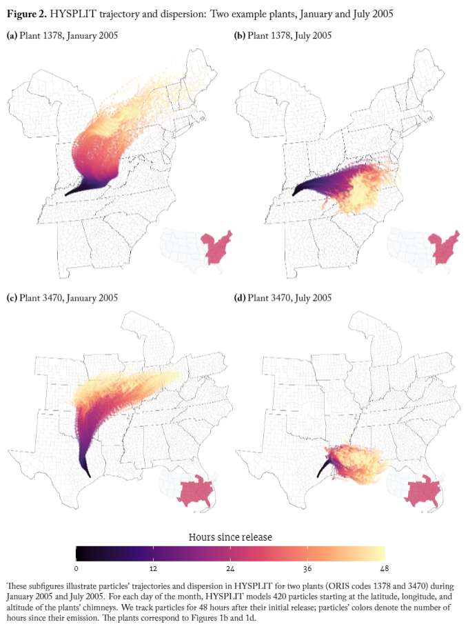
We illustrate the output of HYSPLIT in Figure 2: disperse particle paths for hundreds of particles originating at a specific EGU’s longitude-latitude-height on a given date-time of release.

5.2 Results: Cross-boundary pollution

In Figure 2 it is clear that the two plants’ emissions leave their source counties within a few hours and much of the plants’ emissions leaves their source states within 24 hours of being released. This quick departure from the source counties and states occurs in both January and July. However, Figure 2 also highlights the fact that pollution transport’s distance and direction may vary greatly by season (even within a plant).

Transporting pollution away from sources

To formalize these insights, for each coal plant we calculate the share of emissions that have left the plant’s county/state for each hour after the initial release. We separately calculate these plant-hour shares by administrative unit (county vs. state), month ( January vs. July), and pollutant (NOx vs. SO2). For example, in January 2005, we calculate 32.9% of NOx emissions from coal plant “3470” (depicted in Figure 2c) that have left the plant’s county 1 hour after being release (none of these NOx emissions have left Texas 1 hour after release). Four hours after release (still for plant 3470 in January 2005): 94.6% of NOx emissions have the the plant’s county, and 11.0% have left the plants state. As Figure 1d illustrates, plant 3470 is located upwind of much of its county and even more of its state (Texas), so it is reasonable that it would take time for its emissions to leave both units. For plants more strategically located—e.g., plant 1378 in Figure 1b is ideally located to reduce in-county emissions—most emissions leave the county nearly immediately: 1 hour after release, 69.5% of its emission have already left the county.

Figure 8 shows these results for all operating coal plants. The four subplots separate the results by administrative level (top panel (A): county; bottom panel (B): state) and pollutant (left: SO2; right: NOx). The x-axis gives the number of hours that have passed since the initial emissions release; the y-axis is the share of particles that have left the source’s administrative unit. The thin lines in each figure depict individual coal plants’ monthly averages (black for January; light red for July). The heavy lines with dots provide the average across plants for each hour—weighted by the mass of emissions.

The implications from Panel A of Figure 8 are clear: for most coal plants in the US, nearly all of the plants’ pollution leaves their home counties within 6 hours of the release. This is true in both seasons, but the departure is even faster in winter months (with their, on average, stronger winds). Panel B paints a similar picture for emissions’ departure from source states: within 12 hours of release, 50%–85% of emissions have left the state of origin—and for many plants, this number is closer to 90% (again, particularly in the winter). Figure 8 demonstrates that pollution transport—a result of the geography of plant sitings, stack heights, and local meteorology—-creates a substantial wedge between the sources of coal-based emissions and the downwind counties/states receiving the emissions.

Decomposing the sources of local pollution

Inspired by this breadth of pollution transport, we now use HYSPLIT to separate the sources of local coal-based pollution. Specifically, we decompose the total coal-EGU-generated pollution within a county by the sources of that pollution (i.e., whether the sources are in-county or in-state and whether the sources are in attainment with national standards). Note that we first sum all coal-generated emissions that HYSPLIT locates within a county. This sum ignores where the emissions originated—so long as HYSPLIT places the emissions in the given county. We then decompose this sum by the emissions’ sources. In this decomposition, we separate sources from counties that were in attainment of the NAAQS in 2005 vs. sources from non-attainment counties (i.e., violators of at least one standard in 2005). In 2005, 485 counties were out of attainment (i.e., non-attainment) for at least one the six criteria pollutants.²²

Figure 9 illustrates the results of this source-based decomposition with pollution sources separated into five groups: (1) the county’s own emissions, (2) attainment counties within the same state, (3) non-attainment counties within the same state, (4) attainment counties in a different state, and (5) non-attainment counties in a different state. Panel A shows the results of the decomposition for SO2 emissions; Panel B for NOx.

Given our previous finding that nearly all emissions leave their origin county within six hours, it is unsurprising that a very rather small share of a county’s coal-EGU-based emissions comes from the county’s own EGUs.²³ However, it is rather remarkable just how small the share of own-county emissions are relative to other coal-based EGU sources: the own-county shares (in black in Figure 9) range from 1% to 8%. While still small, it is notable that the share of own-county emissions is much larger for non-attainment counties than for attainment counties. This finding is consistent with coal plants’ emissions and/or presences contributing to non-attainment designations. However, on average, the vast majority of coal-EGU-based emissions in non-attainment counties appears to originate in other counties and states.

In fact, across all counties, regardless of attainment state, the vast majority of emissions originate in other states—i.e., 65% to 85% (the sum of the yellow and orange segments in Figure 9). While this result may at first seem mechanical—each county only has one own state and 49 other states—it requires substantial transmission of other states’ emissions. Without sizable cross-boundary transmission, counties and states would pollute themselves and not others. This result again highlights the significance role long-distance transmission of coal-generated emissions plays in local air quality throughout the US.

A final interesting nuance in the results of Figure 9 is the difference between attainment and non-attainment counties (the left and right halves of the figure, respectively). For non-attainment counties, the plurality (41%–50%) of coal-based emissions comes from sources in non-attainment counties in other states—consistent with the EPA successfully designating many of the major pollution sources for non-attainment counties. For attainment counties, a larger share comes from attainment counties in other states (this share is particularly large for NOx). These result again emphasize the importance and regulatory challenges of trans-boundary emissions.

Non-attainment counties and upwind emissions

Figure 9 aggregates across all counties in a given category (month by NAAQS status). This aggregation is quite useful in describing average trends, but it may miss some of the nuance contained in individual counties. To document some of the underlying variation, Table 4 lists the top 10 non-attainment counties in terms of the county’s share of coal-based NOx emissions that come from in-attainment counties (including counties in the same state and in other states). We restrict the set of counties to those with operating coal plants in January and July of 2005, and we separately rank the counties for the two months.

Table 4 reveals that there are many non-attainment counties that have their own coal plants but receive a substantial share of their coal-based NOx emissions from coal plants located within in-attainment counties—both in the same state and in other states. For instance, in January 2005, the coal plant in Fort Bend County in Texas (part of the Houston CBSA) only contributed only 17.8% of the county’s coal-based emissions—29.3% came from in-attainment in-state sources and 48.1% came from in-attainment, out-of-state sources. For the “top” county in July of 2005—Shelby County in Tennessee (which houses Memphis)—only 6.8% of the county’s coal-based NOx emissions originate within the county, while 54.5% originate from in-attainment plants in other states. The counties in Table 4 may contribute to their own emissions problems in ways other than coal-based electricity generation—e.g., mobile sources or other major stationary sources. Regardless, it is still striking how much of these counties’ coal-based NOx emissions come from external, in-attainment sources—particularly given that these counties (1) are in non-attainment with respect to the NAAQS and (2) house their own coal plants.

Case study: Shelby County, TN

Figure 10 portrays the specific challenges of cross-boundary coal-based emissions (here, NOx) for the aforementioned Shelby County, Tennessee in July 2005. In 2005, Shelby County was designated non-attainment due to its violation of the 8-hour Ozone standard of NAAQS.²⁴ Panel A shows all of the coal-plant-generated NOx emissions that eventually arrive in Shelby County during July 2005 (as estimated by HYSPLIT). We draw the paths that the emissions take to Shelby County in grey; non-attainment counties (for 2005) are cross-hashed in red. Shelby County is outlined in bright yellow. The sources of the emissions are located throughout a broad geographic stretching from Texas to Kansas to Indiana to Georgia—and including both attainment and non-attainment counties.

Notably, the emissions that eventually make their way to Shelby County come from a wide range of directions—emphasizing the importance of the temporal variation in meteorology embedded in HYSPLIT. Overall, Panel A emphasizes the importance of considering potentially large regions of the country when attempting to regulate or improve local air quality.

Panel B of Figure 10 zooms in on the region surrounding Shelby County, Tennessee (the “zoomed” area is approximately 900 km east–west and 600 km north–south). Counties’ fill color in Panel B matches their contribution (as a share) to Shelby County’s coal-generated NOxin July 2005. Panel C provides both the legend for the colors and the histogram for the distribution of counties’ shares of contribution to Shelby County’s NOx. Remarkably, though Shelby County had an operating coal plant in 2005 (and was out of attainment), the coal plant in Humphreys County, TN (which was in attainment in 2005) actually contributed more to Shelby County’s NOx than did Shelby County’s own plant. Further, the coal plant in Independence County, AR (also in attainment in 2005) contributed approximately the same amount of NOx emissions to Shelby County as did Shelby County’s own coal plant.²⁵ As suggested by Table 4 and illustrated in Figure 10, the vast majority of the coal-based NOx emissions in Shelby County, Tennessee—a non-attainment county—came from other states, and a majority of its emissions originated from sources in attainment counties.

6 Conclusions

In this paper, we document (1) the geography of US coal plants and emissions and (2) the challenges these geographies pose to a federalist approach to air-quality regulation.

We begin by recording the tendency for electricity generators in the US to locate near county and state borders. Though proximity to water may explain part of this behavior, it cannot explain firms’/governments’ preference for siting coal plants in locations that reduce the area downwind of the plant within its county and/or state. To formally test for this strategic behavior, we develop a simple, non-parametric test that compares the area downwind of the plant to the area upwind (at the county or state level). This test identifies highly significant evidence of strategic siting among coal plants. This strategic behavior is evident whether we consider plants’ siting within their counties, siting within their states, or siting jointly within their counties and states. Natural-gas plants—who face much lower regulatory pressure due to their much lower emissions—provide a natural falsification test. We find no evidence of strategic siting among natural-gas plants. We also find no evidence that the Clean Air Act affected this tendency to strategically site coal plants, with one possible exception. Coal plants in states’ interior counties may have increased strategic siting following the passage of the CAA—the same period in which the share of coal plants sited in interior counties increased.

In short, the US’s federalist approach to environmental policy blankets the country in an overlapping patchwork of county and state authorities. We find significant evidence of a strategic response in an important class of major polluters: coal plants have been sited to reduce plants’ downwind areas within their counties and states.

Using the particle-transport model HYSPLIT, we document just how transportable coal-based emissions are—and how quickly they leave their source counties/states. Within six hours nearly all emissions have left their source counties, and approximately 50% have left their source state. Part of this quick departure from source counties/states is attributable to plants’ proximity to administrative borders. However, other forces are also at work—i.e., coal plants’ tall smokestacks, meteorology, and the general transportable nature of coal plants’ emissions.

These results have important implications for policy. The strategic siting behavior that we document is consistent with a simple model of regulatory avoidance—likely reducing regulatory efficiency. Under the current (federalism-inspired) implementation of the CAA, cross-boundary pollution requires much stronger coordination and effort than pollution that remains within its source county and state. Thus, strategic siting could render air-pollution regulation less successful or more costly (or both). Adding further complexity are (i) the highly transportable nature of coal-based emissions and (ii) the height of coal plants’ smokestacks. Consequently, local and state governments face a complex challenge in monitoring and regulating these plants that strategically site near downwind borders and release highly transportable pollutants from tall smokestacks.

The shapes of some non-attainment areas reflect this complexity—knitting together whole counties with pieces of other counties and “islands” that surround major point sources. For example, consider the Huntington-Ashland non-attainment area (for the 1997 PM2.5 standard) mapped in light orange in Figure 11. The Huntington-Ashland non-attainment area—a single non-attainment area—covers nine counties (5 whole counties; 4 partial counties) across three states (Kentucky, Ohio, and West Virginia). Six of the counties form a contiguous area. The remaining three counties (two in OH; one in WV) are essentially islands that each include multiple coal plants (circled, red dots). Clearly this complex non-attainment area required substantial coordination across counties and states, source-attribution modeling, and federal oversight.²⁶ Combining (i) our evidence of overt strategic siting, (ii) the large spatial scale of pollution transport, and (iii) the considerable complexity visible in the Huntington-Ashland non-attainment area, it is important to consider whether the potential efficiency offered by federalist air-quality policy has actually been realized.

It is possible that strategic siting and emitting could offer potential benefits if firms locate near coastal borders so that winds carry pollution out to sea.²⁷ However, the majority of coal plants are not sited in this manner. Instead, firms and governments appear to find it profitable to site coal plants near borders, and build tall stacks, to reduce the efficiency of pollution monitoring and regulation. Stronger federal (or regional) oversight could potentially diminish these incentives—effectively smoothing out the spatial patchwork of authorities. Instead, many opponents of the CAA push for a reduced federal influence.

The results of this paper suggest additional complexities in a regulatory and monitoring setting already fraught with complexity. A larger federal role may reduce the incentives that create these complexities. While we specifically document strategic siting, our results more broadly emphasize that regulators must be cautious of strategic responses to regulation—particularly for policies that are spatial in nature or create discontinuities. In short, for every policy action, we should anticipate a strategic reaction.

7 Figures

Figure 1. Upwind and downwind areas in “home” county relative to plants

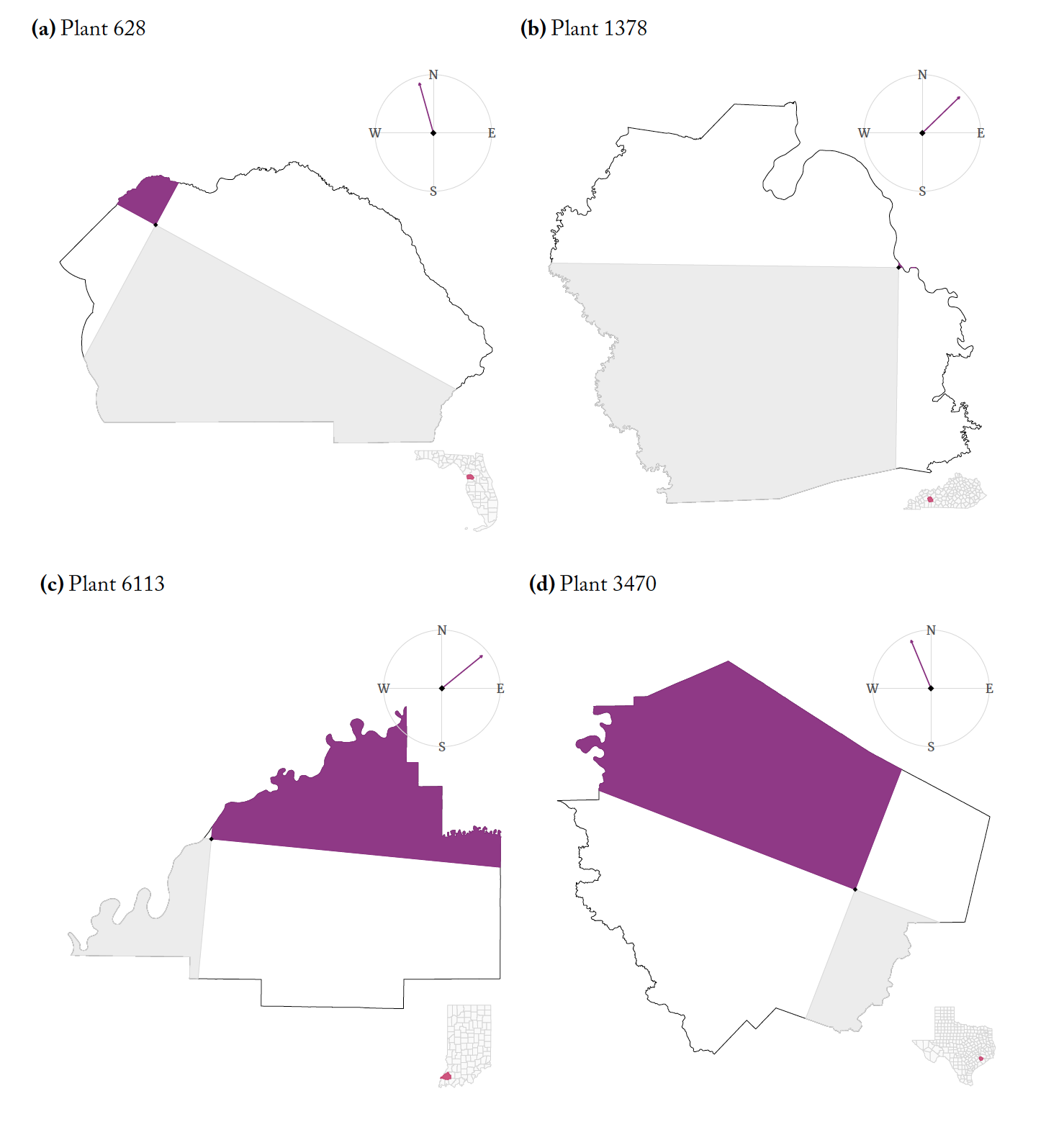
This figure demonstrates upwind and downwind areas for four coal-fueled generators. Dark, purple areas denote the 90-degree upwind area from the plant’s location (the small, black diamond). Light gray refers to downwind areas. The outlined shape depicts the plant’s county; the inset thumbnail highlights the plant within its state. The purple arrow within the compass points in the direction of the plant’s prevailing wind direction (NARR, 2006).

Figure 2. HYSPLIT trajectory and dispersion: Two example plants, January and July 2005

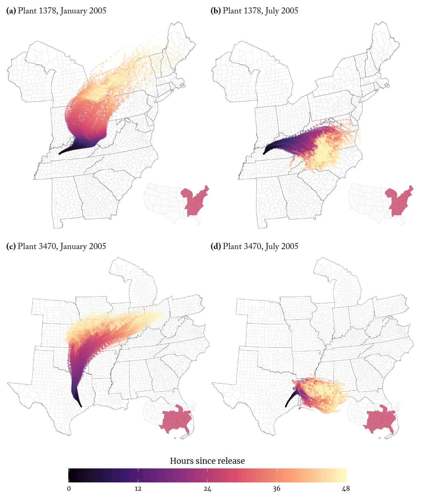
These subfigures illustrate particles’ trajectories and dispersion in HYSPLIT for two plants (ORIS codes 1378 and 3470) during January 2005 and July 2005. For each day of the month, HYSPLIT models 420 particles starting at the latitude, longitude, and altitude of the plants’ chimneys. We track particles for 48 hours after their initial release; particles’ colors denote the number of hours since their emission. The plants correspond to Figures 1b and 1d.

Figure 3. Generators’ distances to country and state borders

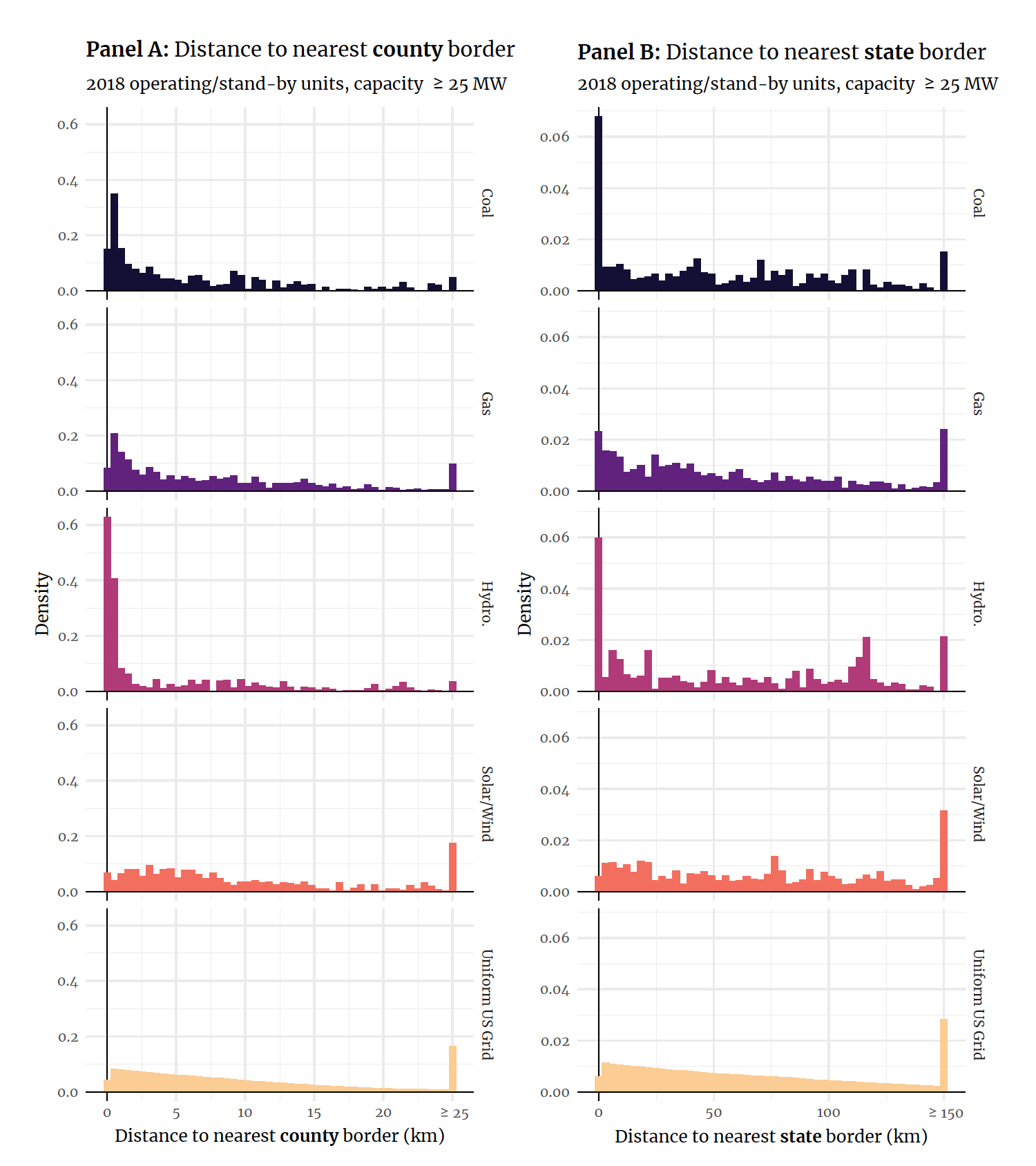
These panels depict the empirical densities of the distributions of EGUs’ distances to their nearest county (Panel A, left) or state (Panel B, right) border. The sample includes all operating and stand-by EGUs with capacities ≥25 MW within the contiguous US in 2018. The first five rows of colored charts above separately produce the densities by fuel category. The final row reveals the density of distance to the nearest border from a uniform grid of points covering the contiguous US.

Figure 4. Generators’ distances to water and capacities

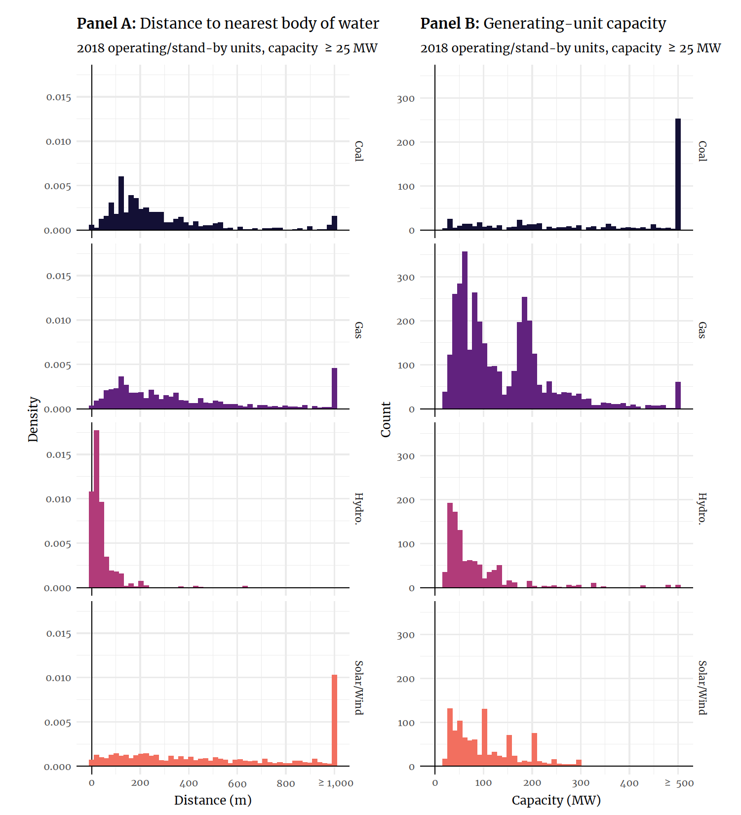
These two panels display the distributions of EGUs’ distances to their nearest body of water (Panel A, left) and EGUs’ generation capacities (Panel B, right) by fuel category (row and color).

Figure 5. Coal and natural-gas plant births by year and by border/interior county

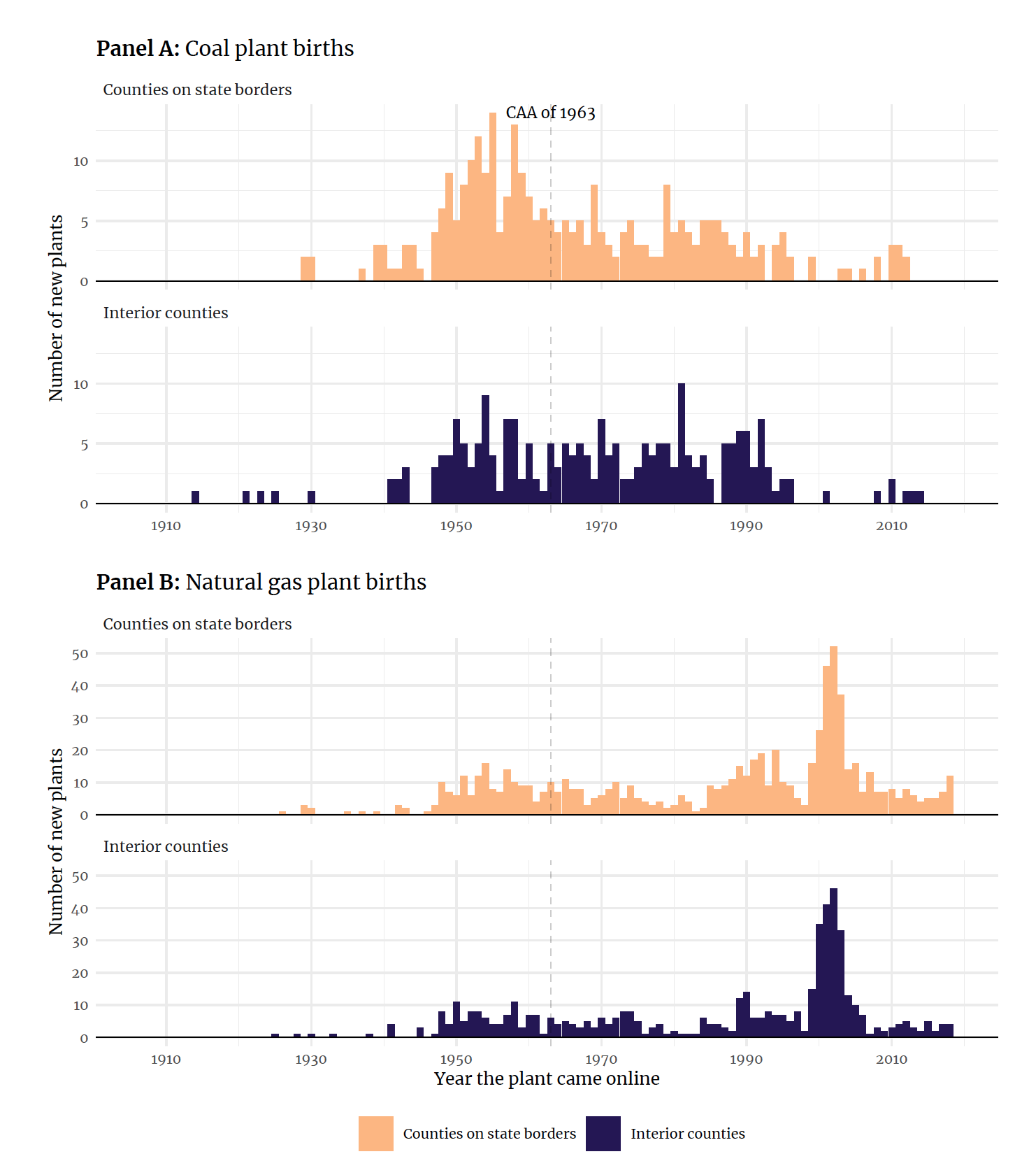
These figures plant the number of plants that came online in each year by (i) the plant’s predominant fuel type (coal in Panel A; natural gas in Panel B) and (ii) whether the plant’s county is on a state border (top; light orange) or is in its state’s entire (bottom; dark blue). Following the Clean Air Act of 1963 (shown by the vertical, dashed line), the share of coal plants built on on state-borders decreased. The CAA of 1963 marked the beginning of increased salience of interstate air-pollution issues.

Figure 6. Shares of county and state borders that intersect water, by state

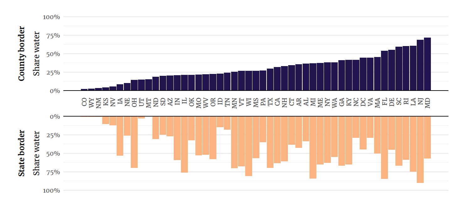
This figure illustrates the share of county borders (top) and state borders (bottom) that intersect with bodies of water, by state. The states are sorted from smallest share of county-borders intersected by water (Colorado) to largest share (Maryland). Alaska and Hawaii are excluded. Figure 7 provides four example states (LA, OR, SC, and SD) from these calculations.

Figure 7. Where county/state borders intersect bodies of water

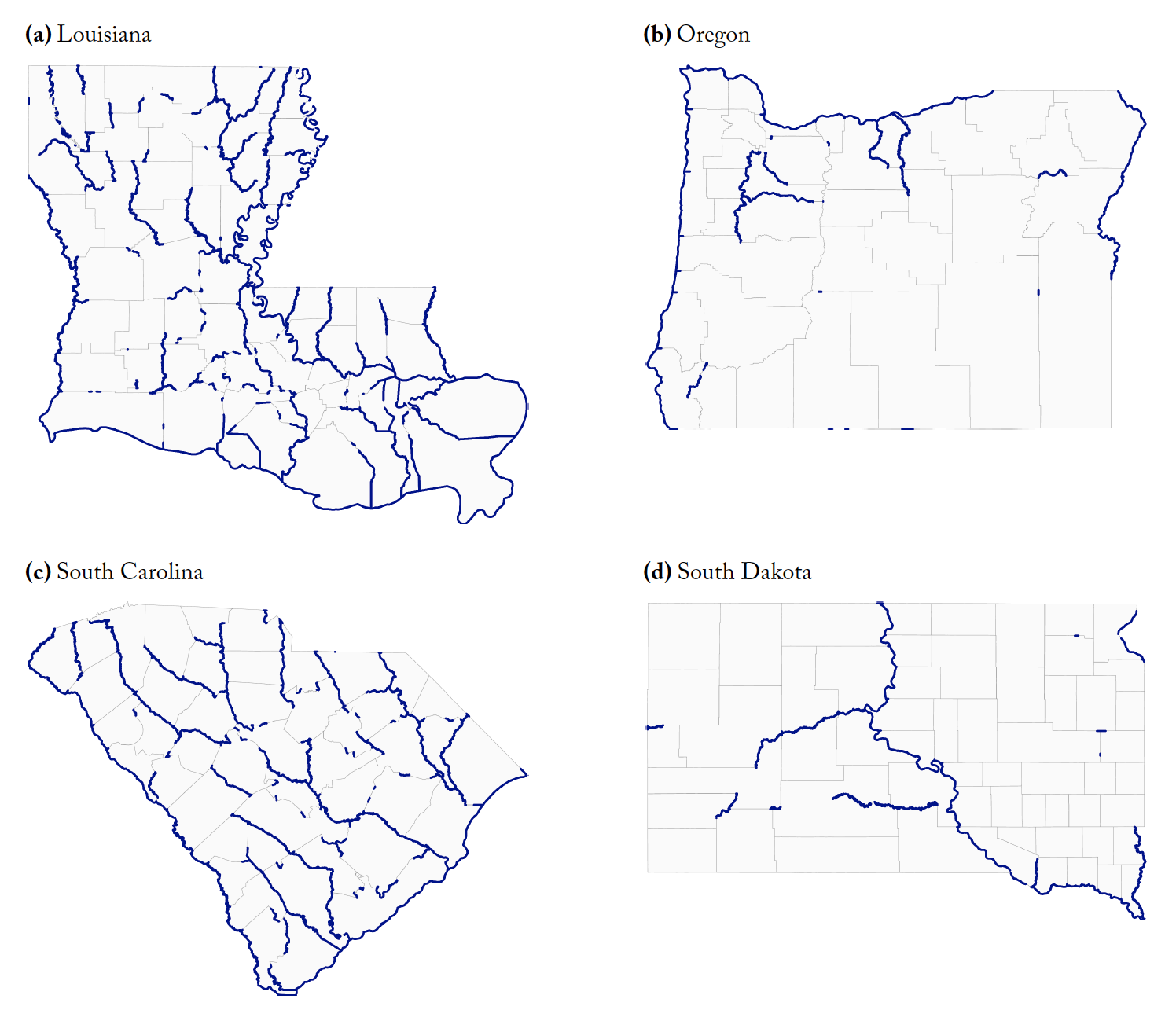
These four subfigures provide examples of the output of our calculations of county and state borders that intersect with bodies of water. Think blue lines denote administrative borders (state and/or county) that intersect with water; thin gray lines depict administrative borders that do not. Overall, our algorithm for detecting borders’ intersections with water appears to be successful.

Figure 8. Share of particles outside of origin county/state by hours since release

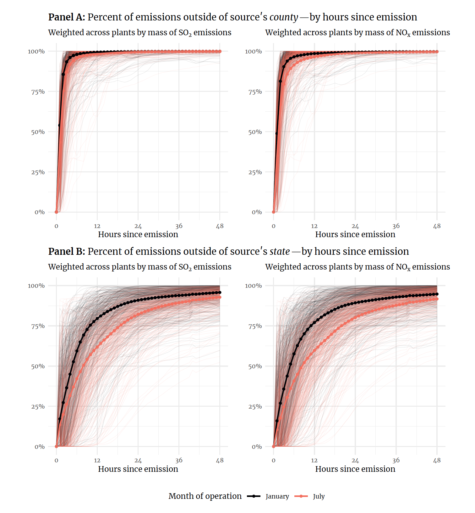
These figures portray the share of coal plants’ emissions that have left plants’ origin counties (top, Panel A) or origin states (bottom, Panel B) by the number of hours that have passed since the particles were released (as modeled by HYSPLIT). Each of the four subfigures contains two months of emissions: January 2005 (black) and July 2005 (light, red). Thin lines depict individual plants in a given month. Thick lines (decorated with hourly points) denote the monthly average across plants (weighted by mass of emissions). The left column weights by SO₂; the right column by NO_x. Differences between the months capture seasonal differences in meteorology and in the distribution of generation. Sample: Coal-fueled generators ≥ 25 MW operating in Jan./July 2005.

Figure 9. Share of particles in a county separated by particles’ sources

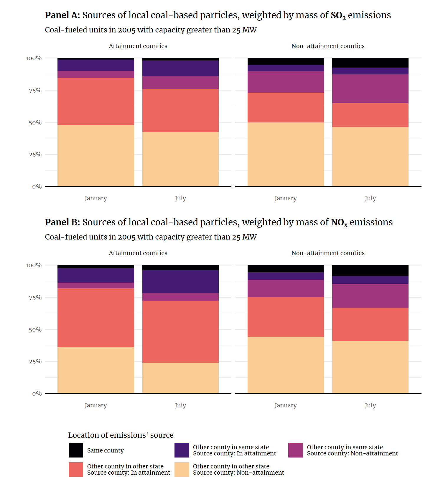
These figures illustrate the source-based decomposition of location, coal-based pollution. They described, on average, where a county’s pollution come from based upon (1) the month (Jan. or July 2005), (2) the county’s attainment status, and (3) the type of particle (SO₂ or NO_x). Particle trajectories come from HYSPLIT. The five colors refer to five categories of pollution sources by the EGU source’s location (described in the legend). Panel A focuses on SO₂ emissions; Panel B on NO_x. Sample: Coal-fueled generators ≥ 25 MW operating in Jan./July 2005.

Figure 10. Illustrating the transport problem: The sources of coal-based NO_x emissions in Shelby County, Tennessee during July 2005

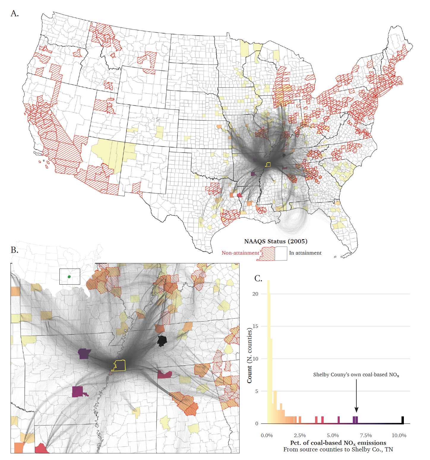
This figure shows the origins, paths, and shares of all coal-plant-based NOx emissions that eventually enter Shelby County, TN during July 2005 (modeled by HYSPLIT). In 2005 Shelby County, TN was in violation of the 8-hour Ozone NAAQS (NO_x is an Ozone precursor). Subfigure A’s grey coal-based NO_x trajectories reveal that the sources of coal-based NO_x emissions in Shelby County include many states (from TX to GA to IL) both in attainment and non-attainment counties. Non-attainment (for any NAAQS) are hashed in red. B zooms in on the region surrounding Shelby County (∼900 km × 600 km). Counties are colored (filled) by the share of coal-based NO_x emissions that they contribute to Shelby County, TN. C provides the legend for B’s colored shares and plots the distribution of these shares—the x axis is the share of Shelby County’s coal-generated NO_x emissions that each county contributes. Despite being ∼200 km from Shelby County, the black-shaded Humphreys County, TN (in attainment for all standards since 1998) accounted for the plurality of coal-generated NO_x emissions in Shelby County, TN during July 2005—i.e., more than Shelby County’s own coal plant.

Figure 11. A “complex” non-attainment area: Huntington-Ashland (WV-KY-OH)

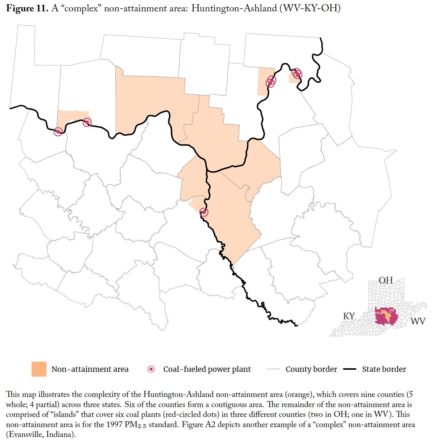
This map illustrates the complexity of the Huntington-Ashland non-attainment area (orange), which covers nine counties (5 whole; 4 partial) across three states. Six of the counties form a contiguous area. The remainder of the non-attainment area is comprised of “islands” that cover six coal plants (red-circled dots) in three different counties (two in OH; one in WV). This non-attainment area is for the 1997 PM_2.5 standard. Figure A2 depicts another example of a “complex” non-attainment area (Evansville, Indiana).

8 Tables

Table 1. Testing strategic location: Comparing up- and down-wind areas for coal and natural gas plants—before and after the Clean Air Act (CAA) of 1963

Table 1

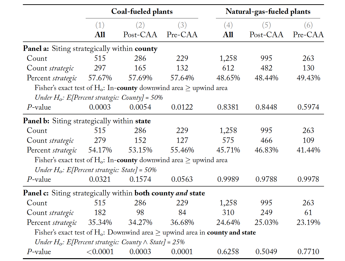
We define a plant’s location as “strategic” if the downwind area within its home county (or state) is less than its upwind area within its home county (or state). We calculate downwind and upwind areas based upon 90-degree right triangles with a vertex at the plant pointing up- or down-wind based upon the locally prevailing wind direction. Figure 1 illustrates this calculation. The columns that reference Post-/Pre-CAA refer to whether the plant’s first year of operation was after or before the Clean Air Act of 1963. Sources: eGRID (2018) and authors’ calculations.

Table 2. Decomposing coal plants’ strategic siting by border and interior counties: Comparing up- and down-wind areas—before and after the Clean Air Act (CAA) of 1963

Table 2

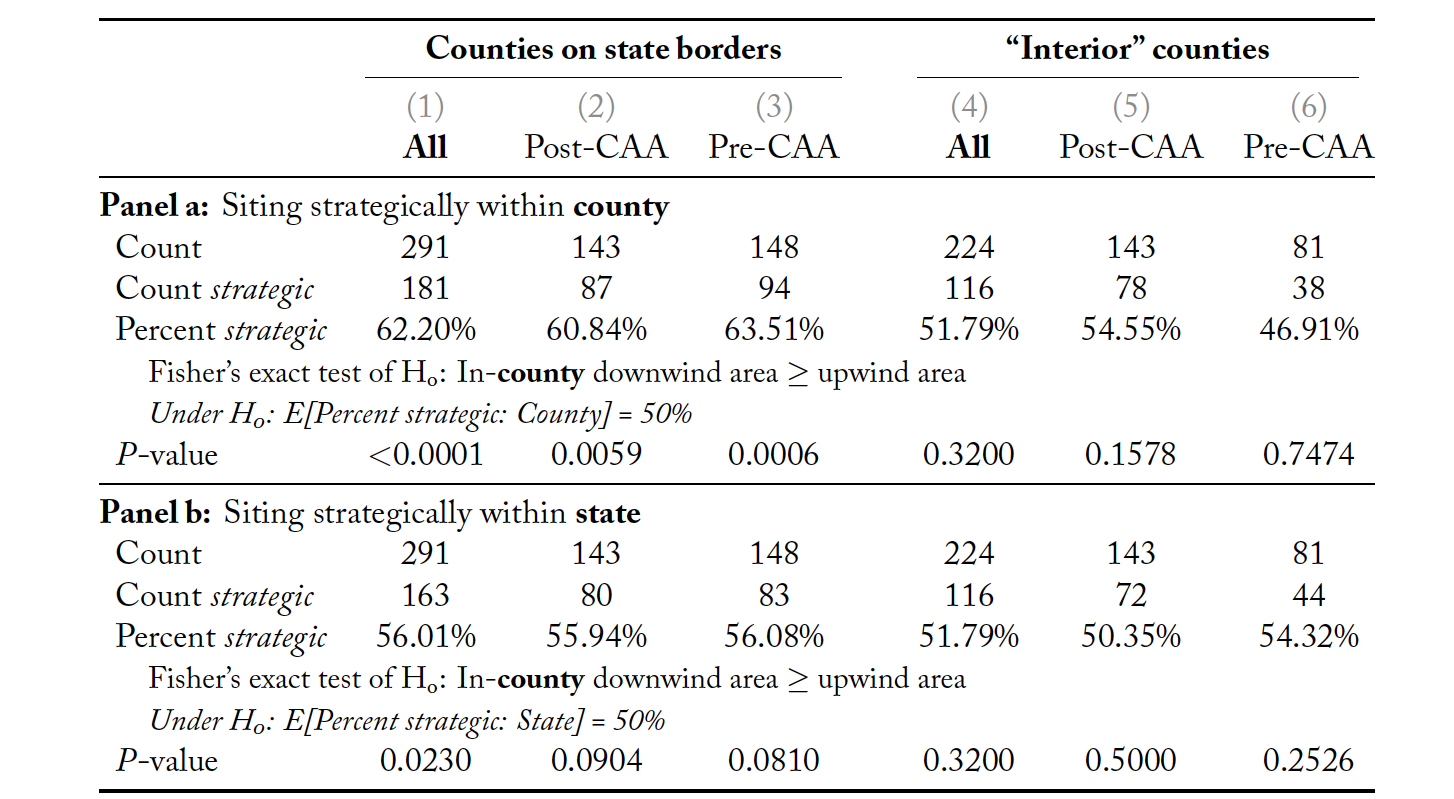
This table documents the differences in the siting of coal plants in counties that touch their states’ borders vs. counties within their states interiors. As above in Table 1, we define a plant’s location as “strategic” if the downwind area within its home county (or state) is less than its upwind area within its home county (or state). We calculate downwind and upwind areas based upon 90-degree right triangles with a vertex at the plant pointing up- or down-wind based upon the locally prevailing wind direction. Figure 1 illustrates this calculation. The columns that reference Post-/Pre-CAA refer to whether the plant’s first year of operation was after or before the Clean Air Act of 1963. Sources: eGRID (2018) and authors’ calculations.

Table 3. Decomposing natural gas plants’ siting by border and interior counties: Comparing up- and down-wind areas—before and after the Clean Air Act (CAA) of 1963

Table 3

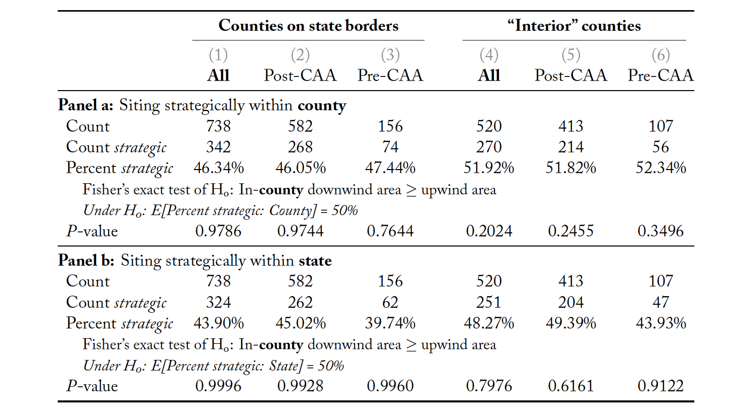
This table documents the differences in the siting of gas plants in counties that touch their states’ borders vs. counties within their states interiors (i.e., this table replicates Table 2 but with natural gas instead of coal). As above in Table 1, we define a plant’s location as “strategic” if the downwind area within its home county (or state) is less than its upwind area within its home county (or state). We calculate downwind and upwind areas based upon 90-degree right triangles with a vertex at the plant pointing up- or down-wind based upon the locally prevailing wind direction. Figure 1 illustrates this calculation. The columns that reference Post-/Pre-CAA refer to whether the plant’s first year of operation was after or before the Clean Air Act of 1963. Sources: eGRID (2018) and authors’ calculations.

Table 4. Top 10 non-attainment counties by share of local coal-based NOx emissions originating from sources in external, in-attainment counties, January and July 2005

Table 4

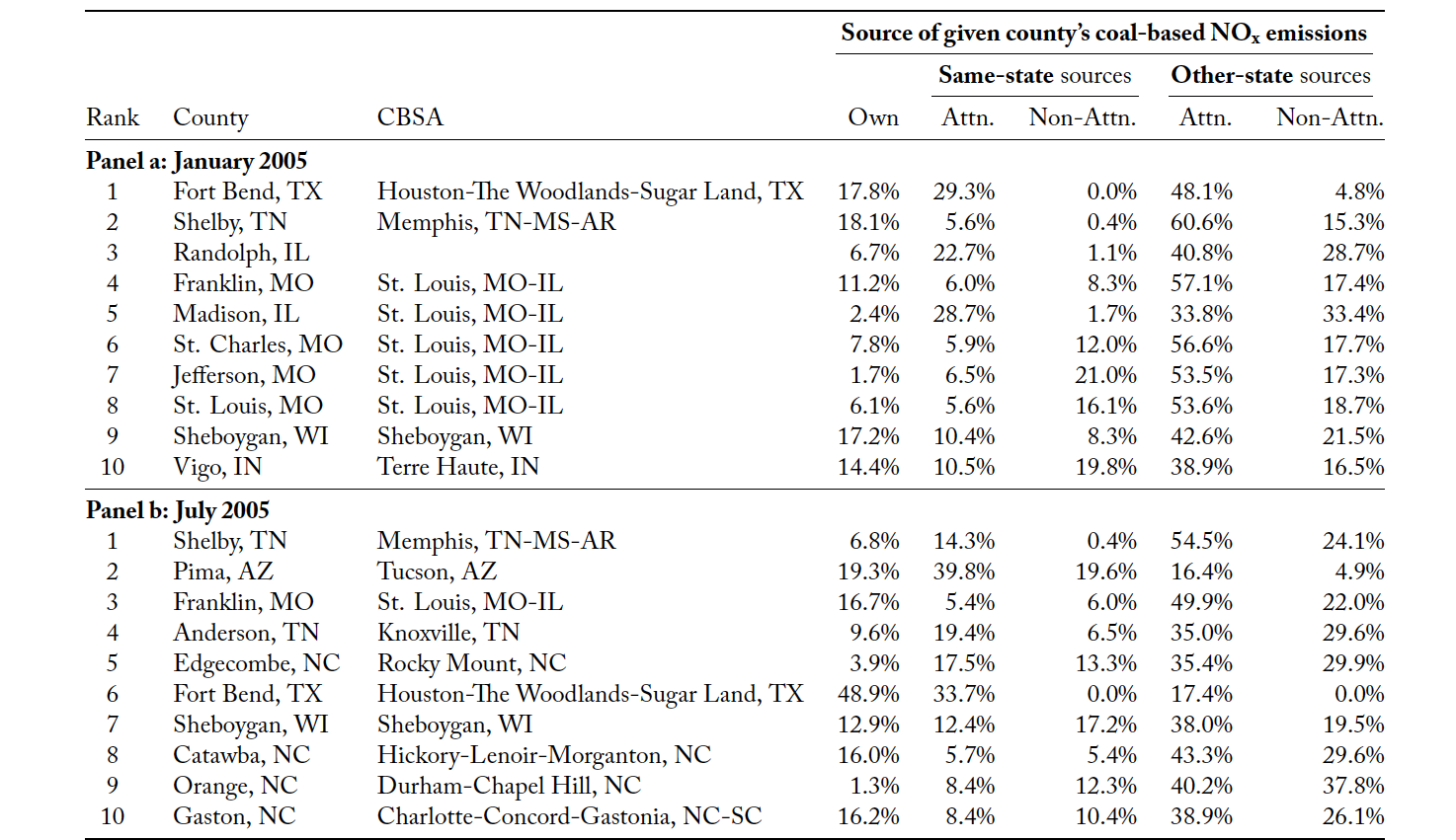
This table highlights how much coal plants in attainment counties may affect air quality in non-attainment counties. We decompose (and rank) each county’s coal-generated NO_x emissions by the source of the emissions (same-state vs. other-state sources) and by attainment status of the source. Attn. and Non-attn. refer to sources in attainment and non-attainment jurisdictions, respectively. Counties in this table meet two criteria: (1) non-attainment counties (2) with non-zero coal generation in the given months. We rank counties by the share of coal-based NO_x originating from in-attainment sources (separately for January/July 2005). These shares are based upon HYSPLIT estimates, as described in the methods.

Appendix

A.1 Appendix: Methods

A.1.1 Border-distance calculations

We first project the plant’s location and the Census shapefiles into the plant’s zone of the Universal Transverse Mercator (UTM) coordinate system. Then we calculate the distance to the plant’s nearest county and state border. We use R’s sf package for these calculations (Pebesma, 2018).

A.1.2 Counterfactual grid

If the county and state borders do not impact or correlate with EGUs’ locations, then EGU’s distances to borders should mirror the overall national distribution of distances to borders.To build this comparison distribution, we cover the contiguous US with a uniform, hexagonal grid of points as illustrated in Appendix Figure A1. The number of grid points is approximately equal to the area covered in square kilometers. We then calculate each point’s distances to the nearest county border and the nearest state border.²⁸ This process produced a nationally representative distribution (for the contiguous US) of distances to state and county borders using a uniform grid of approximately 7.91 million points.²⁹ This distribution represents the expected distribution of EGUs’ distances to borders if they were sited in a manner that ignores borders and features that correlate with borders.

The last row of Figure 3 depicts the distribution of distance-to-nearest-border for the uniform grid covering the US. This grid’s distribution demonstrates that it is not the case that all points in the United States are near borders. Only 8% of the US (area-wise) sits with 1 kilometer of a county border (36% within 5 km; 62% within 10 km). For state borders, only 1.1% of the US sits within 1 kilometer (6% within 5 km; 11% within 10 km). These numbers stand in stark contrast to the distributions of EGUs.

A.1.3 Borders and water

We calculate the share of each county’s and state’s borders that intersect bodies of water in four steps. First, we convert each administrative unit’s linear boundaries into a series of points with 50-meter spacing. Second, we calculate the distance to the nearest body of water for each of these boundary points (if the boundary point is within a body of water, then the distance is zero). These bodies of water cover all rivers, lakes, and coastlines including in the US Census’s TIGER/Lines shapefiles discussed in Data. Third, we designate a boundary point as including water if the nearest body of water is less than 50 meters. This step allows for near misses in the Census geography files without including too many false positives. Finally, we smooth this includes water indicator variable using a moving-window average of all boundary points within a 2.5 kilometer radius of the given boundary point. This final step allows neighboring boundary points to vote on whether the boundary indeed intersects water—e.g., a single, spurious includes water will be overwhelmed by non-water neighbors. The final product is a series of points with 50-meter spacing covering all county and state borders in the contiguous US—with each point measuring whether the boundary substantively intersects with water.

A.1.4 EGUs and water

To calculate the distance to the nearest body of water, we include all bodies of water contained in the US Census’s areas of water, linear water, and coastline shapefiles, (US Census Bureau, 2016b). After merging these calculated distances with eGRID’s EGU characteristics, we build the distribution of
distance-to-water for each fuel category.

A.1.5 HYSPLIT

The R packages splitr, hyspdisp, and dispersR were extremely helpful in developing our computational approach—as was GNU Parallel (Tange, 2011).

A.2 Appendix: Figures

Figure A1. Example of grid for distance calculation

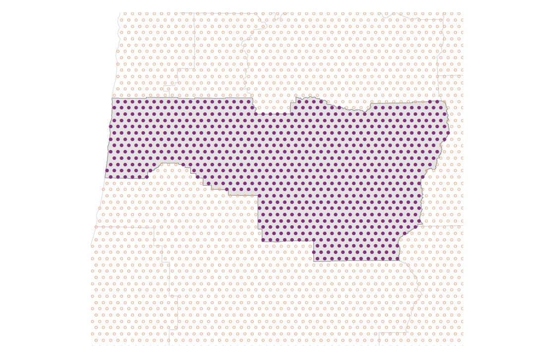
This figures illustrates the uniform grid within our nearest-border calculation. All dots (open and closed) are part of the uniform grid. Closed, dark purple dots are within Lane County, Oregon. We then calculate the shortest distance from each dot to borders of Lane County and of Oregon.

To test whether the distribution of EGUs’ distances to nearest borders is consistent with random sampling from the national grid we employ a simple, non-parametric, Kolmogorov-Smirnov test. The
Kolmogorov-Smirnov test is designed to test whether the empirical distribution of a sample statistically differs from a known distribution, which is exactly our goal of this exercise: does the distribution of the EGUs differ from the national distribution?³⁰ We focus on five major fuel categories: coal, gas, hydropower, and other renewables (wind and solar). For each fuel category, we test whether its EGUs’ distances to county (or state) borders statistically differ from the distribution of grid points’ distances to borders (the grid described above).³¹ The results are displayed in A1.

Figure A2. A “complex” non-attainment area: Evansville, IN

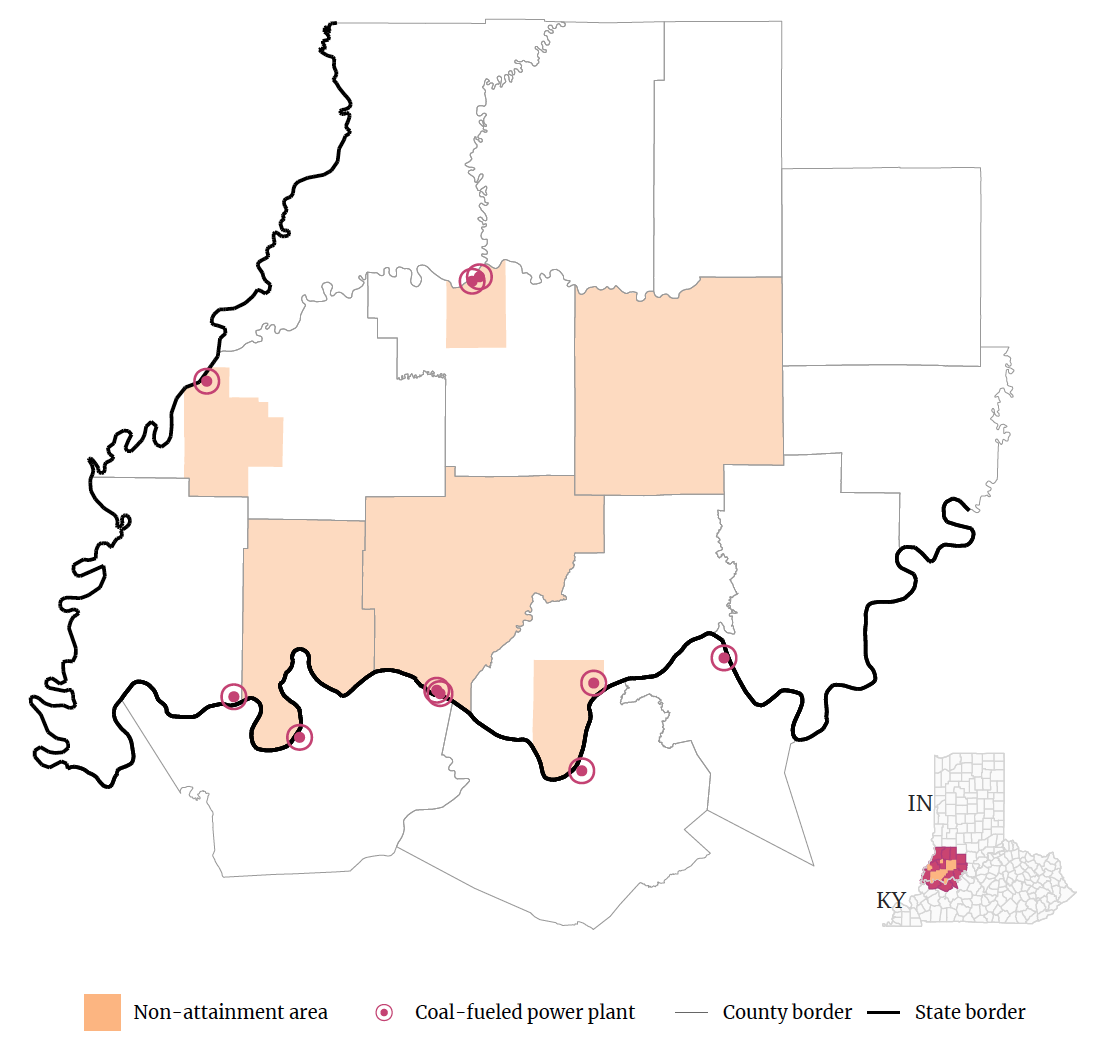
This map illustrates the complexity of the Evansville, Indiana non-attainment area (orange), which covers six counties (3 whole; 3 partial) within Indiana (along its borders with Kentucky to the south and Illinois to the west). Six of the counties form a contiguous area. The remainder of the non-attainment area is formed by islands in three counties that cover nearby coal plants (circled, red dots). As with Figure 11, the non-attainment area is for the 1997 PM_2.5 standard.

A.3 Appendix: Tables

Table A1. Testing EGUs’ border distances relative to uniform US grid border distance

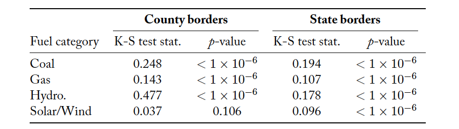
The columns labeled K-S test stat. contain Kolmogorov-Smirnov test statistics testing EGUs’ distances to borders against the distribution of distance-to-border built by our uniform national grid. We conduct the tests by EGU fuel category (rows) and administrative level (county and state). The p-values correspond to the adjacent Kolmogorov-Smirnov test statistic.

The K-S test resoundingly rejects that null hypothesis that the EGUs’ distributions mirror the grid’s distribution for each combination of administrative level (county or state) and fuel category (coal, gas, hydro, or solar/wind) with one exception. As one may guess from Figure 3, the one exception is the distance from solar and wind generators to the nearest county border. This distribution fails to reject the null with a p-value of approximately 0.106 (and a K-S test statistic of 0.037). Except for the solar and wind generators’ distances to county borders, we observe overwhelming evidence that EGUs are disproportionately sited near county and state borders—particularly for coal and hydropower units. This observation emphasizes the complexity of monitoring and regulating emissions from EGUs.

References

Becker, Randy and Henderson, Vernon (2000). “Effects of Air Quality Regulations on Polluting Industries”. Journal of Political Economy 108.2, 379–421.

Browning, Dominique (2020). “Don’t Celebrate Earth Day. Fight for It.” New York Times. (Visited on 07/14/2020).

CAMD (2020). US EPA, Clean Air Markets Division.

Congressional Research Service (2012). Air Quality: EPA’s 2012 Proposed Changes to the Particulate Matter (PM) Standard, R42671. Tech. rep. – (2013). 2006 National Ambient Air Quality Standards (NAAQS) for Fine Particulate Matter (PM2.5): Designating Nonattainment Areas, R40096. Tech. rep.

Conover, William J. (1971). Practical Nonparametric Statistics. New York: John Wiley & Sons.

Draxler, Roland, Stunder, Barbara, Rolph, Glenn, Stein, Ariel, and Taylor, Albion (2020). HYSPLIT User’s Guide. 5th ed. NOAA Air Resources Laboratory.

Draxler, Roland R. and Hess, G. D. (1998). “An Overview of the HYSPLIT(4) Modelling System for Trajectories”. Australian Meteorological Magazine 47.4, 295–308.

Edelman, Sidney (1966). “The Law of Federal Air Pollution Control”. Journal of the Air Pollution Control Association 16.10, 523–525.

Emissions & Generation Resource Integrated Database (2018). Emissions & Generation Resource Integrated Database. (Visited on 07/03/2020).

Feldman, Stacy (2010). “Report: Business Groups Say Clean Air Act Has Been a ‘Very Good Investment’”. Reuters. (Visited on 07/14/2020).

Fisher, R. A. (1934). Statistical Methods for Research Workers. 5th ed. Edinburgh: Oliver & Boyd.
– (1935). The Design of Experiments. 8th ed. New York: Hafner Publishing Company, Inc.

Grainger, Corbett and Ruangmas, Thanicha (2017). “Who Wins from Emissions Trading? Evidence from California”. Environmental and Resource Economics 71.3, 703–727.

Grainger, Corbett, Schreiber, Andrew, and Chang, Wonjun (2018). “Do Regulators Strategically Avoid Pollution Hotspots when Siting Monitors? Evidence from Remote Sensing of Air Pollution”. University of Madison–Wisconsin Working Paper.

Gray, Wayne B. (1997). “Manufacturing Plant Location: Does State Pollution Regulation Matter?” NBER Working Paper No. 5880.

Groom, Nichola (2019). “Six U.S. States Sue Trump’s EPA over Interstate Smog Pollution Rule”. Reuters. (Visited on 07/14/2020).

Henneman, Lucas R.F., Choirat, Christine, Ivey, Cesunica, Cummiskey, Kevin, and Zigler, Corwin M. (2019). “Characterizing population exposure to coal emissions sources in the United States using the HyADS model”. Atmospheric Environment 203, 271–280.

Henneman, Lucas R.F., Choirat, Christine, and Zigler, Corwin M. (2019). “Accountability Assessment of Health Improvements in the United States Associated with Reduced Coal Emissions Between 2005 and 2012”. Epidemiology 30.4, 477–485.

Henneman, Lucas R.F., Mickley, Loretta, and Zigler, Cory (2019). “Air Pollution Accountability of Energy Transitions: The Relative Importance of Point Source Emissions and Wind Fields in Exposure Changes”. Environmental Research Letters.

Hernandez-Cortes, Danae and Meng, Kyle C. (2020). “Do Environmental Markets Cause Environmental Injustice? Evidence from California’s Carbon Market”. NBER Working Paper No. 27205.

Imbens, Guido W. and Rubin, Donald B. (2015). Causal Inference for Statistics, Social, and Biomedical Sciences: An Introduction. Cambridge: Cambridge University Press, 57–82.

Jeppesen, Tim and Folmer, Henk (2001). “The confusing relationship between environmental policy and location behaviour of firms: A methodological review of selected case studies”. The Annals of Regional Science 35.4, 523–546.

Jeppesen, Tim, List, John A., and Folmer, Henk (2002). “Environmental Regulations and New Plant Location Decisions: Evidence from a Meta-Analysis”. Journal of Regional Science 42.1, 19–49.

Levinson, Arik (1996). “Environmental Regulations and Manufacturers’ Location Choices: Evidence from the Census of Manufactures”. Journal of Public Economics 62.1-2, 5–29.

List, John A., Millimet, Daniel L., Fredriksson, Per G., and McHone, W. Warren (2003). “Effects of Environmental Regulations on Manufacturing Plant Births: Evidence from a Propensity Score Matching Estimator”. Review of Economics and Statistics 85.4, 944–952.

Mani, Muthukumara, Pargal, Sheoli, and Huq, Mainul (1997). “Does Environmental Regulation Matter? Determinants of the Location of New Manufacturing Plants in India in 1994”. World Bank Working Paper 1718.

McConnell, Virginia D. and Schwab, Robert M. (1990). “The Impact of Environmental Regulation on Industry Location Decisions: The Motor Vehicle Industry”. Land Economics 66.1, 67–81.
McDermott, Grant R. (2020). “Hydro power. Market might.”

Mesinger, Fedor, DiMego, Geoff, Kalnay, Eugenia, Mitchell, Kenneth, Shafran, Perry C., Ebisuzaki, Wesley, Jović, Dušan, Woollen, Jack, Rogers, Eric, Berbery, Ernesto H., Ek, Michael B., Fan, Yun, Grumbine, Robert, Higgins, Wayne, Li, Hong, Lin, Ying, Manikin, Geoff, Parrish, David, and Shi, Wei (2006). “North American Regional Reanalysis”. Bulletin of the American Meteorological Society 87.3, 343–360.

Millimet, Daniel L. and List, John A. (2003). “A Natural Experiment on the ‘Race to the Bottom’ Hypothesis: Testing for Stochastic Dominance in Temporal Pollution Trends”. Oxford Bulletin of Economics and Statistics 65.4, 395–420.

Monogan III, James E, Konisky, David M, and Woods, Neal D (2017). “Gone with the Wind: Federalism and the Strategic Location of Air Polluters”. American Journal of Political Science 61.2, 257–270.

North American Regional Reanalysis (2006). North American Regional Reanalysis. (Visited on 07/03/2020).

Oates, Wallace E. (1972). Fiscal Federalism. NY: Harcourt. – (2002). A Reconsideration of Environmental Federalism. Ed. by John A. List and Aart de Zeeuw. UK: Edward Elgar.

Pebesma, Edzer (2018). “Simple Features for R: Standardized Support for Spatial Vector Data”. The R Journal 10.1, 439–446.

Preonas, Louis (2019). “Market Power in Coal Shipping and Implications for U.S. Climate Policy”.
Working paper.

Ren, Xinrong, Hall, Dolly L., Vinciguerra, Timothy, Benish, Sarah E., Stratton, Phillip R., Ahn, Doyeon, Hansford, Jonathan R., Cohen, Mark D., Sahu, Sayantan, He, Hao, Grimes, Courtney, Salawitch, Ross J., Ehrman, Sheryl H., and Dickerson, Russell R. (2017). “Retracted: Methane Emissions from the Marcellus Shale in Southwestern Pennsylvania and Northern West Virginia Based on Airborne Measurements”. Journal of Geophysical Research: Atmospheres 122.8, 4639–4653.

Revesz, Richard L. (1996). “Federalism and Interstate Environmental Externalities”. University of Pennsylvania Law Review 144.6, 2341–2416.

Ryaboshapko, Alexey, Bullock, O. Russell, Christensen, Jesper, Cohen, Mark, Dastoor, Ashu, Ilyin, Ilia, Petersen, Gerhard, Syrakov, Dimiter, Artz, Richard S., Davignon, Didier, Draxler, Roland R., and Munthe, John (2007). “Intercomparison Study of Atmospheric Mercury Models: 1. Comparison of Models with Short-Term Measurements”. Science of The Total Environment 376.1-3, 228–240.

Sanders, Linley (2018). “EPA to be Sued Over Power Plant Pollution Spreading Into Neighboring State”.
Newsweek. (Visited on 07/14/2020).

Sergi, Brian, Azevedo, Inês, Davis, Steven J., and Muller, Nicholas Z. (2020). “Regional and County Flows of Particulate Matter Damage in the US”. Environmental Research Letters 15.10, 104073.

Shadbegian, Ronald and Wolverton, Ann (2010). “Location Decisions of U.S. Polluting Plants: Theory, Empirical Evidence, and Consequences”. U.S. EPA Working Paper #10-05.

Stein, A. F., Draxler, R. R., Rolph, G. D., Stunder, B. J. B., Cohen, M. D., and Ngan, F. (2015). “NOAA’s HYSPLIT Atmospheric Transport and Dispersion Modeling System”. Bulletin of the American Meteorological Society 96.12, 2059–2077.

Stein, Ariel F., Rolph, Glenn D., Draxler, Roland R., Stunder, Barbara, and Ruminski, Mark (2009). “Verification of the NOAA Smoke Forecasting System: Model Sensitivity to the Injection Height”.
Weather and Forecasting 24.2, 379–394.

Stunder, Barbara J. B., Heffter, Jerome L., and Draxler, Roland R. (2007). “Airborne Volcanic Ash Forecast Area Reliability”. Weather and Forecasting 22.5, 1132–1139.

Tange, O. (2011). “GNU Parallel – The Command-Line Power Tool”. ;login: The USENIX Magazine 36.1 (February), 42–47.

Tessum, Christopher W., Hill, Jason D., and Marshall, Julian D. (2017). “InMAP: A Model for Air Pollution Interventions”. PLOS ONE 12.4. Ed. by Juan A. Añel, e0176131.

Tiebout, Charles M. (1956). “A Pure Theory of Local Expenditures”. Journal of Political Economy 64.5, 416–424. U.S. Environmental Protection Agency (2013a). Clean Air Act, Section 110 (42 U.S.C. 7401). Tech. rep. – (2013b). Clean Air Act, Section 126 (42 U.S.C. 7426). Tech. rep. – (2017a). 1990 Clean Air Act Amendment Summary: Title I. (Visited on 07/13/2020). – (2017b). Evolution of the Clean Air Act. (Visited on 07/14/2020). – (2017c). Green Book National Area and County-Level Multi-Pollutant Information. (Visited on 06/25/2020). – (2017d). NAAQS Table. (Visited on 07/13/2020). – (2018). 2014 National Emissions Inventory, v2, Technical Support Document. Tech. rep. – (2020a). Basic Information about Air Quality SIPs. (Visited on 11/30/2020). – (2020b). Overview of the Cross-State Air Pollution Rule (CSAPR). (Visited on 07/14/2020).

U.S. Government Accountability Office (2011). Information on Tall Smokestacks and Their Contribution to Interstate Transport of Air Pollution (GAO-11-473). Tech. rep. Institution.

United States Congress (90th) (1968). “The Air Quality Act of 1967”. Journal of the Air Pollution Control Association 18.2, 62–71.

United States Senate, Committee on Public Works, Staff Report (1963). A Study of Pollution—Air.
Tech. rep. Washington DC: 88th, Congress, 1st Session.

US Census Bureau (2016a). Cartographic Boundary Shapefiles. (Visited on 10/15/2020).
– (2016b). TIGER/Lines Shapefiles. (Visited on 07/14/2020).

Volcovici, Valerie (2018). “Delaware to Sue EPA over Upwind Air Pollution”. Reuters. (Visited on 07/14/2020).

Wang, Yuzhou, Bechle, Matthew J., Kim, Sun-Young, Adams, Peter J., Pandis, Spyros N., Pope, C. Arden, Robinson, Allen L., Sheppard, Lianne, Szpiro, Adam A., and Marshall, Julian D. (2020). “Spatial Decomposition Analysis of NO2 and PM2.5 Air Pollution in the United States”. Atmospheric Environment 241.

Woerman, Matt (2020). “Market Size and Market Power: Evidence from the Texas Electricity Market”.
Working paper.

Wolverton, Ann (2009). “Effects of Socio-Economic and Input-Related Factors on Polluting Plants’ Location Decisions”. The B.E. Journal of Economic Analysis & Policy 9 (1).

Zou, Eric (2020). “Unwatched Pollution: The Effect of Intermittent Monitoring on Air Quality”.

Downwind and Out: The Strategic Dispersion of Power Plants and Their Pollution

Executive Summary

Resources

Focuses

States

House/Senate Committees

Federal Agencies

Testing strategic location: Comparing up- and dow1 Introduction

2 Institutions

3 Data

4 Strategic siting and the geography of US electricity plants

4.1 EGUs’ distances to borders and water

4.2 A test for regulatory avoidance

4.3 Results: Strategic plant siting

5 Cross-border pollution and the geography of emissions

5.1 HYSPLIT

5.2 Results: Cross-boundary pollution

6 Conclusions

7 Figures

8 Tables

Appendix

A.1 Appendix: Methods

A.2 Appendix: Figures

A.3 Appendix: Tables

References

Executive Summary

Resources

Related Publications

Related News

Related Blogs

Focuses

States

House/Senate Committees

Federal Agencies

Testing strategic location: Comparing up- and dow1 Introduction

2 Institutions

3 Data

4 Strategic siting and the geography of US electricity plants

4.1 EGUs’ distances to borders and water

4.2 A test for regulatory avoidance

4.3 Results: Strategic plant siting

5 Cross-border pollution and the geography of emissions

5.1 HYSPLIT

5.2 Results: Cross-boundary pollution

6 Conclusions

7 Figures

8 Tables

Appendix

A.1 Appendix: Methods

A.2 Appendix: Figures

A.3 Appendix: Tables

References