How Policing Incentives Affect Crime, Measurement, and Justice

Adamson, Jordan; Rentschler, Lucas

1 Introduction

Recent events have returned police violence to the forefront of policy debates. While many researchers are focused on the magnitude of racial prejudice or simply assume police are a public good, we still know little about what incentives lead to better or worse policing. In this study, we create a principal-agent model to examine how different carrots and sticks for police officers affect multiple aspects of criminal justice (such as the number of innocents who are punished and the number of criminals who are not).

In our model, officers allocate finite resources to protect specific locations (either spatially displacing crime or deterring it altogether) or on investigation (which affects the probabilities of punishing the innocent and letting the guilty go free). While most theories assume that police act in the public interest, painting “the enforcement apparatus—police, courts, prosecutors, and legislature—as a philosopher-king, with imperfect knowledge but only the best of motives” (Friedman 1999), our model allows us to explore the multidimensional response to different incentives.¹

We develop a rich strategic environment in which civilians can either produce or attempt to steal by targeting the property of others. An officer allocates their budget between defending civilian property (patrolling) and increasing the probability that thieves are punished and producers are not (investigating). Police and thieves interact over space, with officers seeking to catch criminals and criminals hiding from detection. In equilibrium, officers and thieves randomize their location choices, which endogenizes the probabilities of arrest and conviction. This spatial interaction allows us to examine the effects of different policing incentives while addressing the critique by Tsebelis (1989) that economists have been “mistaking the equilibrium mixed strategy of the opponent for a probability distribution.”

A truth table of criminal justice is derived which summarizes the equilibrium number of true and false positives (and negatives) for both innocent and guilty civilians. This lets us examine whether different incentives push toward a police state (with large proportions of the population being arrested, guilty or not) or pull away from mayhem (where only the most heinous and clear-cut crimes are prosecuted).

We then analyze the two main incentives for police laid out by Becker and Stigler (1974): “one penalizes malfeasance and other signs of weak enforcement; the other, which we think is preferable, rewards success.” First, we show that appropriately balancing these two incentives will minimize theft (the focus of most economists). Stronger penalties for wrongful arrest can reduce false positives at the cost of an increase in crime. Conversely, weaker penalties lead to a reduction in the quality of investigations which, undercuts deterrence and increases crime. Thus, if officer accountability is sufficiently low, an increase will decrease crime while simultaneously decreasing the number of false convictions. Second, we show when changes in police incentives will lead to an increased clearance rate and an increase in crime (i.e., an often-used metric of police performance can “improve,” despite an increase in both crime and false positives). Third, we show what the ratio of false positives and negatives (a central legal tenet but peripheral to the economic study of crime) misses in criminal justice outcomes.

Police incentives have long been recognized as an important determinant of criminal justice outcomes. In examining policies to prevent police abuse, Devi and Fryer (2020) state “one way forward is to design a set of incentives such that we increase the penalties of unconstitutional policing and, simultaneously, lower the probability of being wrongfully accused when controversial interactions occur.” While most have argued police performance incentives would lead to bad outcomes (e.g., Landes and Posner 1975; Friedman 1999), and there is evidence that high-powered incentives can create problems (Baicker and Jacobson 2007; Dharmapala, Garoupa, and McAdams 2016), it does not follow that we should abolish all police incentives. For example, stricter punishment might lead officers to avoid risky investigations (Shi 2009). Building on Holmstrom and Milgrom (1987), Holmstrom and Milgrom (1991), and Hart, Shleifer, and Vishny (1997), our model is a first step in clarifying what incentives are effective—or just what is needed to avoid reprehensible outcomes.

While we primarily focus on the effects of police incentives, our model provides an important building block for understanding the spatial distribution of crime, which has been largely neglected in the literature. The seminal paper by Levitt (1997) acknowledged that “it is impossible to determine… whether the observed decrease in crime in central cities in response to increased police represents a geographical reallocation of crime rather than a true reduction.” This shortcoming has still not been addressed in the “causal effects of police” literature, and the mixed empirical results as to how important geographical spillovers and displacement effects are hard to interpret.²

Moreover, we also incorporate false arrests into our framework, building on the literature on punishment accuracy (Kaplow and Shavell 1994; Persson and Siven 2007; Rizzolli and Stanca 2012; Markussen, Putterman, and Tyran 2016; Lando and Mungan 2018; DeAngelo and McCannon 2016). Thus, we endogenize both the level and spatial distribution of crime, as well as the probability of arrest and the accuracy of punishment. We also extend the literature by considering an entire population rather than a representative civilian—which leads to a crucial distinction between the rates and absolute numbers of different types of errors. As a whole, we significantly extend the “general-equilibrium model” of policing (Ehrlich 1973; İmrohoroğlu, Merlo, and Rupert 2000) under a common theoretical framework so that each may inform the other.

In particular, we show how a source of scarcity largely ignored—that police departments allocate their budget to both patrolling and investigating—is crucial to understanding criminal justice outcomes.³ Although officer investigation reduces the chance an innocent is punished, the overall number of false positives can be increasing with investigation due to a reduction in boots on the ground. Moreover, both false positives and crime can be increasing alongside improving metrics. We show how and when improvements in police performance metrics are associated with higher crime and worse justice outcomes—i.e., systematic mismeasurement.

There is almost no economic theory underpinning the metrics that empiricists use, and we help fill this gap. Although there have been some detractors (e.g., Cook 1979; Sparrow 2015), “evidence based” policing has become dominant in both policing and economic studies. Yet, the main source of such crime data: the Uniform Crime Report, warns

“These rough rankings provide no insight into the numerous variables that mold crime in a particular town, city, county, state, tribal area, or region. Consequently, they lead to simplistic and/or incomplete analyses that often create misleading perceptions adversely affecting communities and their residents.”⁴

We highlight a particular problem with the prominent position of evidence based policing. Its advocates argue that policy changes must be driven by data, which restricts attention to observable metrics. We provide reason to suspect this emphasis on observable metrics may cause more harm than good at the margin. Specifically, the unobservability of false positives can lead policy-makers to neglect the costs of inaccurate punishment. For example, the widespread practice of using the clearance rate to evaluate policy can lead to situations in which it appears that policing outcomes are improving, when in fact they are worsening. As a result, the emphasis on clearance rates may not just be problematic for applied research on policing, but also for the people who live with the resulting policies. For example, the Miami Herald (Rabin, Weaver, and Ovalle 2018) reported on such a case:

“If they have burglaries that are open cases that are not solved yet, if you see anybody black walking through our streets and they have somewhat of a record, arrest them so we can pin them for all the burglaries,” one cop, Anthony De La Torre, said in an internal probe ordered in 2014. “They were basically doing this to have a 100% clearance rate for the city.”

3 Theory

There are $n+1$ risk-neutral players who play a one-shot game. One player is an officer and $n\geq 2$ players are civilians. Each civilian chooses between production and theft, while the officer attempts to prevent thefts. If civilian $i$ produces, he earns a payoff of $Y_i \geq 0$ . (Own productivity is private information, but the joint distribution of productivities is common knowledge.) For convenience, civilians are indexed according to their productivity, where $i=1$ is the most productive and $i=n$ is the least productive. The probability that a share of the population has productivities weakly below $c\in[0,\infty)$ is given by $F_Y(c)>0$ . We assume that $F_Y$ is differentiable with density $f_Y$ .

Each civilian owns a $\Lambda \times \Lambda$ square, which we refer to as his property, as well as a steal token. When a civilian attempts to steal from another, he does so by placing his steal token at any point on the other civilian’s property.⁵ If this point is not defended by the officer, then a quantity $s>0$ is stolen.

To defend locations on the civilian properties, the officer uses defend tokens, each of which is a $\Omega \times \Omega$ square (with $\Omega \leq \Lambda$ ). Each of these tokens can be placed on any of the civilian properties. If a steal token is placed on a point covered by a defend token, then the attempted theft is unsuccessful, and an “investigation” is launched, which may result in one of the civilians being fined an amount $\psi>0$ . For any investigation, the likelihood that the culprit is subsequently punished depends on the resources police have allocated to investigation. The officer allocates a fixed budget $e$ between the number of defend tokens $d$ and the quality (or accuracy) of investigation $a$ ; $e \geq a+d$ . The officer faces a trade-off between either preventing theft by increasing $d$ , or accurately punishing theft by increasing $a$ .⁶

In any investigation, the victim is never suspected, but each of the other innocent civilians face a punishment probability of $\rho_{I}(a) \in [0,1]$ . The culprit faces a punishment probability of $\rho_{C}(a)\in [0,1]$ . (Note that a civilian is considered “innocent” if they are punished for a crime they did not commit, even if they are in fact a thief.) These individual probability functions can depend on other parameters (such as the size of the population) but are constrained by the probability that anyone is punished, $\rho_{A}(a)=[n-2]\rho_{I}(a) + \rho_{C}(a) \in [0,1]$ . (E.g., when $\rho_{A}$ is fixed, the only effect of increasing the quality of investigation, $a$ , is to concentrate the probability of punishment on the culprit rather than an innocent civilian.) Moreover, the probability functions are continuously differentiable and exhibit weak diminishing-returns:

(1) $\begin{eqnarray*} \rho_{C}^{'} \geq 0, &\rho_{I}^{'} \leq 0, & \rho_{A}^{'} \geq 0 \nonumber \\ \rho_{C}^{''} \leq 0, &\rho_{I}^{''} \geq 0, & \rho_{A}^{''} \leq 0 . \end{eqnarray*}$

The officer receives a bonus of $B>0$ for cleared crimes (interruption events that end with punishment). The officer also expects a reprimand of $R>0$ for false convictions: each case is reviewed with probability $\theta$ and the officer pays a penalty $P$ if an innocent civilian was arrested, so $R=P \theta$ . Further, we assume these incentives are not extreme: $B/R \in \left[1, \frac{[n-2][\rho_{I}(0) - e\rho_{I}^{'}(0)]}{ \rho_{A}(0) - e\rho_{A}^{'}(0) }\right]$ . We also assume that, $s$ , the amount stolen when thieves are successful, is large enough that, in expectation, not all crime can be deterred: $s>\frac{\left(\psi\rho_{C}(e-d) \frac{d}{n}\left(\frac{\Omega}{\Lambda}\right)^{2}\right)}{\left(1-\frac{d}{n}\left(\frac{\Omega}{\Lambda}\right)^{2}\right)}$ for any $d$ .

3.1 Thieves Hide and Officers Seek

Consider the location choices of the officer with a fixed number of defend tokens, $d$ , and a fixed number of people stealing, $n_{S}$ . Equilibrium behavior on a given property involves the officer and thieves mixing over all locations. If there were a location that was never covered, then the thief would go there with certainty, and the officer would never interrupt thieves. If there were a location that was always covered by the officer, then the thief would never go there, and again the officer would never interrupt the thief. Similarly, neither the thief nor the officer can even favour a location. Using a derivation familiar in stochastic geometry, the equilibrium probability of an interruption with uniform mixing can be calculated in terms of areas.

Lemma 1 (lone-mixing). For a single thief and an officer with a single defend token, the equilibrium probability of an interruption between the steal token and the defend token on a single property is $[\Omega/\Lambda]^2$ .

Proof. See Appendix B.

A similar result holds when looking \textit{across}, rather than \textit{within} properties. When the benefits and costs of stealing (for civilians) and defense (for officers) are constant across players, the officer and thieves will assign equal probability mass to each of the properties where there is a potential for thievery. If the officer deviates, then thieves will go to properties that have lower defenses. If thieves deviate, the officer will go to the properties where they expect more thieves. If there were only one thief, they steal only from the other $n-1$ civilians. Since the officer is equally uncertain about who the single thief is, then he still equally defends all $n$ properties. When there is more than one thief, stealing occurs on all $n$ civilian properties, and the officer again equally defends all properties.⁷

Lemma 2 (group-mixing). For n_S people stealing and an officer with a single defend token, the equilibrium expected number of interruptions between the steal token and the defend token is $\phi = [\Omega/\Lambda]^2 n_{S}/n$ .

Proof. See Appendix B.

For $d$ defend tokens, the equilibrium expected number of interruptions is $d \phi > 0$ . In the current paper, our focus is on the effects of policing incentives ( $B$ and $R$ ). As such, consideration of more general spatial settings (which nest the above setup as a special case) is relegated to Appendix C.

3.2 Officers Patrol and Investigate, Civilians Produce or Steal

The officer expects to earn

(2) $\begin{eqnarray*} \mathbb{E}[\Pi_{O}] &=& B [ [n-2]\rho_{I}+\rho_{C} ] d\phi - R [n-2]\rho_{I} d \phi \nonumber \\ &=& d\phi \left[ [B-R][n-2]\rho_{I}+ B \rho_{C} \right] . \end{eqnarray*}$

When more civilians steal, $\phi$ increases and expected clearance bonuses and reprimands increase by equal amounts. The officer exhausts the budget, $a=e-d$ , and chooses $d \in [0,e]$ to maximize expected earnings. If incentives are not extreme,⁸ the officer’s optimal choice is implicitly defined by

(3) $\begin{eqnarray*} d^{*}&=& %\frac{ \left[1-\frac{1}{B/R}\right][n-2] \rho_{I}+ \rho_{C} }{ \left[1-\frac{1}{B/R}\right][n-2]\rho_{I}^{'}+ \rho_{C}^{'} } %= \frac{ \frac{B}{R} \rho_{A} - [n-2]\rho_{I}}{\frac{B}{R} \rho_{A}^{'} - [n-2]\rho_{I}^{'}} \frac{ \left[\frac{B}{R}-1\right] \rho_{A} + \rho_{C}}{\left[\frac{B}{R}-1\right] \rho_{A}^{'} +\rho_{C}^{'}} \end{eqnarray*}$

This unique choice determines the equilibrium probabilities of punishing the culpable, $\rho_{C}^{*}=\rho_{C}(e-d^{*})$ , and the innocent, $\rho_{I}^{*}=\rho_{I}(e-d^{*})$ . In turn, these probabilities determine civilian choices of whether to produce or steal.

Civilians steal when theft has a higher expected return than production. The expected profit for civilian $i$ when producing is $i's$ own wealth, $\overline{Y_{i}}$ minus the amount successfully stolen, $S_{i}$ , minus the expected amount from being incorrectly fined, $I_{i}$ , plus the amount produced, $Y_{i}$ . The expected profit for civilian $i$ when stealing from $j$ is $\overline{Y_{i}}-S_{i}-I_{i}$ , plus the expected amount gained from theft, $s [1- d/n [\Omega/\Lambda]^2 ]$ , minus the expected penalty from being correctly accused, $\psi \rho_{C} d/n [\Omega/\Lambda]^2$ . The amount $\overline{Y_{i}} - S^{i} - I^{i}$ does not affect the decision to produce or steal, which implies that civilians face a constant cutoff;

(4) $\begin{eqnarray*} \mathbb{E}[\Pi_{i}(\text{Produce}) - \Pi_{i}( \text{Steal from } j)] &=& Y_{i} - c(d) , \\ %&=& \left[\overline{Y_{i}} - S^{i} - I^{i} + Y_{i} \right] - %\left[\overline{Y_{i}} -S^{i} - I^{i} + s \left[1- \frac{d}{n} \left( \frac{\Omega}{\Lambda} \right)^2 \right] \end{eqnarray*}$

(5) $\begin{eqnarray*} %- F \rho_{C} \frac{d }{n} \left( \frac{\Omega}{\Lambda} \right)^2 \right], \\ c(d) &=& s - \frac{d \left[s+\psi \rho_{C} \right] }{n} \left( \frac{\Omega}{\Lambda} \right)^2. \end{eqnarray*}$

Thus, any civilian with $Y_i\leq c(d^*) \equiv c^*$ steals. The expected number of thieves is $n_S^{*} \equiv F_{Y}\left(c^* \right)n$ .

Proposition 3 (equilibrium). The Bayes-Nash equilibrium strategies are for the officer to choose d^∗ defend tokens (implicitly defined) to randomly patrol all locations with equal probability, and the civilians with Y_i ≤ c^∗ to steal by randomizing locations such that the probability of being caught is equal across all locations.

Proof. The unique optimal choice for the officer is d^∗, which does not depend on F_Y (c^∗). Then, since F_Y (c^∗) is a function of d^∗, all civilians with Y_i ≤ c^∗ steal. Combined with Lemmas 1 and 2, all defend tokens and steal tokens are mixed uniformly across all locations. (In the section on parametric examples, Figure 1 depicts equilibrium and the underlying forces.)

These micro strategies have important distributional effects on aggregate outcomes. In equilibrium, the probability that an individual thief is caught is $\frac{d^*}{n} \left( \frac{\Omega}{\Lambda} \right)^2$ . Combined with the probabilities of punishment, this determines the expected number of civilians who steal, as well as the number of civilians falsely punished or incorrectly let go. The probability that an individual thief is correctly punished is $\frac{d^*}{n} \left( \frac{\Omega}{\Lambda} \right)^2 \rho_{C}^*$ . The expected number of thieves on other maps (except the focal map, as victims are not punished) is $n_{S}^{*} -1 - \frac{n_{S}^{*}}{n}$ .⁹ This means that the probability an individual thief is incorrectly punished is $\left( n_{S}^{*} -1 - \frac{n_{S}^{*}}{n} \right) \frac{d^*}{n} \left( \frac{\Omega}{\Lambda} \right)^2 \rho_{I}^*$ . Similarly, the probability an individual producer is punished is $\left( n_{S}^{*} - \frac{n_{S}^{*}}{n} \right) \frac{d^*}{n} \left( \frac{\Omega}{\Lambda} \right)^2 \rho_{I}^*$ . The aggregate implications weight these probabilities by the numbers of thieves or producers, and are reported in the truth table of criminal justice:

Truth table of criminal justice

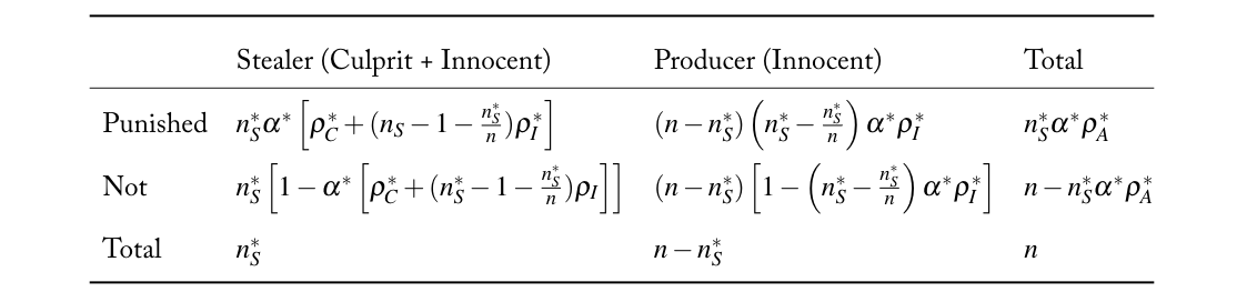
Note: Each cell shows the either the expected number of stealers or producers that are or are not punished. Recall the equilibrium punishment probabilities are $\rho_I^*$ for an innocent, $\rho_C^*$ for the culprit, and $\rho_A^*$ for anyone. Note that a civilian is “innocent” if they are incorrectly punished—this includes producers who are punished and thieves who are punished for the wrong crime. The probability an individual thief is caught is denoted as $\alpha^*=\frac{d^*}{n}\left(\frac{\Omega}{\Lambda}\right)^2$ . The equilibrium number of thieves is $n_S^*$ (out of $n$ civilians).

The equilibrium behavior summarized in this table has important implications for the way economic theorists, applied econometricians, and legal theorists have studied policing. In doing so, we are able to evaluate whether an isolated analysis of one or two aspects of the table is informative in isolation; the answer is generally no. Focusing on just one or two elements can be seriously misleading because the table is irreducible from a welfare perspective. It is the minimal relevant summary for any welfare function that is decreasing in crime and false positives (independent of crime). In what follows, we do not presume a specific social welfare function, only that crime and false convictions are both undesirable.¹⁰ We provide three negative results for crime, measurement, and justice to illustrate a central issue within each field’s typical focus. In the interest of brevity, we limit our discussion to comparative statics of $B/R$ .¹¹ In doing so, we highlight how this truth table of criminal justice can holistically inform policy reform.

4 Insights for Crime, Measurement, and Justice

Officer incentives affect the amount of resources allocated to investigation, which in turn affects the probability that thieves are interrupted ( $d^{*}\phi^{*}$ ) the probability of being punished conditional on being interrupted ( $\rho_{C}^{*}$ ) and thus the income cutoff for thievery ( $c^{*}$ ). This, as we will show, affects the key elements of the table of truth injustice. Three corollaries collect our general propositions into the main points we want to stress, which are then represented visually in Section 5.

How the officer responds to incentives will be crucial, so first note that patrolling increases (and investigation decreases) with a larger ratio of bonuses to reprimands; $\frac{\partial d^{*}}{\partial B/R} \geq 0$ .¹² On the other hand, the income distribution affects the equilibrium share of the population stealing, $F_{Y}\left(c^*\right)$ and how many people are affected by the incentives, $f_{Y}(c^*)$ , but not the level of $B/R$ which minimizes crime. Specifically, crime is minimized when $\frac{ \text{d} n_{S}^{*}/n}{ \text{d } B/R} = f_{Y}(c^*) \frac{\text{d } c^*}{\text{d } B/R}=0$ , where $\frac{\text{d } c^*}{\text{d } B/R} = \frac{-1}{n}\left( \frac{\Omega}{\Lambda}\right)^2 \left[ s + \psi \rho_{C}^{*}-\psi d^{*}\rho_{C}^{*'} \right] \frac{\partial d^{*}}{\partial B/R}$ . The crime rate is convex in $B/R$ , and is minimized by weighing the deterrence that comes from both the probability of apprehension and the accuracy of punishment.

Lemma 4 (minimum). The level of crime is convex in $B/R$ , and is minimized with moderate incentives;

(6) $\begin{eqnarray*} B/R^{\bullet} &:& d^{*} = \frac{ \psi \rho_{C}^{*}+ s}{ \psi \rho_{C}^{*'}}. \end{eqnarray*}$

Proof. The first order condition for an optimum is $\frac{\text{d } c^*}{\text{d } B/R} = 0$ , which defines $B/R^{\bullet}$ . Then, due to the diminishing marginal returns shape of $\rho_{C}$ , the population share of thieves is always convex in $B/R$ : $\rho_{C}^{*''} \leq 0 \leq 2 [\rho_{C}^{* '}]^2 / [\phi \rho_{C}^{*} + s]$ . Thus, $B/R^{\bullet}$ is the minimum.

When there are larger rewards for clearances ( $B/R$ is high) officers devote fewer resources to making sure the punishment is accurate and more resources to patrolling and arresting civilians. As a result, a larger bonus will lead many thieves to be interrupted ( $d^*$ being high has a high “apprehension effect”). However, this deterrence can be undercut by the high probability of inaccurate punishment ( $\rho_{C}^{*}$ being low has a low “accuracy effect”). A larger bonus will lead to more interruptions but also more inaccurate punishments. On the other hand, when officers expect larger penalties for false conviction, $B/R$ is low, and they spend fewer resources on active patrolling and more on collecting evidence. This will lead to few inaccurate punishments but also fewer interruptions. Maximal deterrence occurs when neither the apprehension effect nor accuracy effect is too strong.

These results have important implications for policy. Opponents of increased police accountability often argue that increasing police accountability ( $R$ ) would lead to an increase in crime since officers would best respond with less aggressive policing. We show that the opposite can be true: increased accountability can induce better investigation and increase crime deterrence. On the other hand, opponents of pay-for-performance argue that high powered incentives ( $B$ ) leads to a “race to the bottom.” We show that the opposite can be true: increased bonuses can induce more patrolling and increase the deterrence of crime. These remarks will seem paradoxical to some scholars and pundits, but that is because officer incentives are discussed as if they had a constant linear effect. Our model highlights the trade-offs that lead the equilibrium level of theft to be non-monotonic in $B/R$ : excessive officer incentives—either to clear crimes or avoid reprimands—can actually increase thefts by causing too few apprehensions or too inaccurate punishments.

From Lemma 4, it is also clear that the income distribution plays an important role in crime. Empirically, poverty and income inequality are driving factors of crime. (See Hsieh 1993 for a historical review of income inequality and crime, and Pridemore 2011 for evidence that poverty is the driving factor.) These factors are intimately connected in our theory.

Corollary 5 (inequality). Inequality affects crime and the efficacy of police in reducing crime.

Proof. Consider an income distribution with a single scale parameter, $\sigma$ , that determines the dispersion of incomes. There is a first order effect of inequality on theft; $d n_{s}^{*} /d \sigma = d F_{Y}(c^{*} |\sigma) / d \sigma$ . There is also a cross-effect of inequality on policing efficacy; $d^2 n_{s}^{*}/ [d \sigma d c^{*}] = d f_{Y}(c^{*} |\sigma) / d \sigma$ .

Remark. More disperse incomes shifts each quantile away from 0, thus creating fewer thieves. (When holding the average income constant, however, more dispersion can increase crime.) Moreover, when more of the population has incomes close to the cutoff, small changes in officer incentives can lead to large changes in the level of theft. With a relatively poor marginal thief, increasing income dispersion shrinks $f_{Y}(c^{*})$ and lessens the effects of officer incentives.

Many inequality scholars discuss inequality as if the mean where unchanged but, for non-negative distributions, increasing the dispersion also increases the central tendency. The confounding of mean and variance can be seriously misleading. (E.g., the mean and the variance are the same in a Poisson distribution, where “infinite inequality” does not sound so bad when it is phrased as “infinite average incomes.”) To theoretically address the joint determination of mean and variance, one can consider a “compensating” formulation that allows for comparative statics on inequality while holding average incomes constant. E.g., $d f_{Y}(c^{*} |\sigma)/ d \sigma = \partial f_{Y}(c^{*} |\sigma)/ \partial \sigma + \partial f_{Y}(c^{*} |\sigma)/ \partial \mu_{c}(\sigma) ~ \partial \mu_{c}(\sigma) / \partial \sigma$ , where the $\mu_{c}(\sigma)$ is a compensated location parameter that holds mean incomes constant.

Despite crime being only one of several important attributes of criminal justice, economic theorists almost exclusively focus on deterrence and crime minimization. This focus neglects false positives, which feature prominently in any evaluation of the performance of a criminal justice system:

(7) $\begin{eqnarray*} FP &\equiv& (n-n_{S}^{*}) n_{S}^{*} \frac{n-1}{n^2} \left(\frac{\Omega}{\Lambda}\right)^{2} d^{*} \rho_{I}^{*}. %FN &\equiv& n_{S} \left[1- \frac{d}{n} \left(\frac{\Omega}{\Lambda}\right)^{2} \left[ \rho_{C}+\left(n_{S}-1-\frac{n_{S}}{n}\right) \rho_{I}\right] \right]. \end{eqnarray*}$

Provided that, in equilibrium, the entire population is not expected to steal, and there is a positive probability of false convictions, then the level of false convictions is increasing in $B/R$ .

Theorem 6 (crime). At $B/R^{\bullet}$ , crime is minimized but false positives are already increasing.

Proof. False convictions are strictly increasing at $B/R^{\bullet}$ when $n_{S}^{*}<n$ and $\rho_{I}^{*}>0$ . Evaluated at $B/R^{\bullet}$, $\frac{d n_{S}^{*}}{d B/R}=0$ . Then

(8) $\begin{eqnarray*} \frac{d FP }{ d B/R } &=&\frac{n-1}{n^2} \left(\frac{\Omega}{\Lambda}\right)^{2} \left[ (n-2n_{S}^{*})\rho_{I}^{*} d^{*} \frac{d n_{S}^{*}}{d B/R} + n_{S}^{*}(n-n_{S}^{*})\left( \rho_{I}^{*} -\rho_{I}^{*'} d^{*} \right)\frac{\partial d^{*}}{\partial B/R} \right] \end{eqnarray*}$

simplifies to $\frac{d FP }{ d B/R } = n_{S}^{*}(n-n_{S}^{*})\frac{n-1}{n^2} \left(\frac{\Omega}{\Lambda}\right)^{2} [\rho_{I}^{*} -\rho_{I}^{*'} d^{*} ] \frac{\partial d^{*}}{\partial B/R}$ . Given $n_{S}^{*}<n$ and $\rho_{I}^{*}>0$ , all terms are strictly positive except for $\rho_{I}^{*'} \leq 0$ . Thus $\frac{d FP }{ d B/R }$ is positive at $B/R^{\bullet}$ . From proposition 4, we also know that crime is at a minimum.

Remark. Increased accountability (or reduced pay-for-performance) reduces the probability of apprehension but increases the probability of punishing the culprit. These opposing effects lead theft to be minimized with moderate officer incentives. However, civilians may care about being falsely punished in and of itself (the central concern of legal theory). This means increasing officer incentives to further reduce crime may be undesirable.

Turning attention to the applied econometric analysis of policing, many studies rely on observed clearance rates as a measure of police efficiency (Paré, Felson, and Ouimet 2007; Bove and Gavrilova 2017; Blanes i Vidal and Kirchmaier 2017; Mastrobuoni 2019; Mastrobuoni 2020). Several criminologists have called this measure into question (Nagin, Solow, and Lum 2015; Pogarsky and Loughran 2016) and Gillen, Snowberg, and Yariv (2019) recently showed that measurement errors have more substantive effects than previously realized in an OLS framework.

We first provide a precise theoretical calculation that demonstrates how the clearance rate depends on police incentives. In equilibrium the clearance rate of crimes (total punished / total thieves) is

(9) $\begin{eqnarray*} CR = \frac{d^*}{n} \left(\frac{\Omega}{\Lambda}\right)^{2} \rho_{A}^{*}. % d^{*}\phi^{*} F_{Y}(c^{*}) \frac{n^2}{n-1} \left[ \rho_{C}^{*} + (n-2 - F_{Y}(c^{*})) \rho_{I}^{*} \right] \end{eqnarray*}$

Notice the clearance rate is not affected by the income distribution. Further, police incentives have an unambiguous effect on this clearance rate.

Theorem 7 (measurement). For $B/R > (B/R)^{\bullet}$ , both the clearance rate and crime are increasing in $B/R$ .

Proof. First, the clearance rate is always increasing in $B/R$ . Note that $\frac{ d CR}{d B/R} = \frac{1}{n} \left(\frac{\Omega}{\Lambda}\right)^{2} [\rho_{A}^{*} - \rho_{A}^{*'} d^{*}] \frac{\partial d^{*}}{d B/R}$ . Because $\rho_{C}^{*} \leq \rho_{A}^{*}$ and $\rho_{C}^{*'} \geq \rho_{A}^{*'}$, $\frac{\rho_{C}^{*'}}{\rho_{C}^{*}} \geq \frac{\rho_{A}^{*'}}{\rho_{A}^{*}}$ . This implies $\frac{\rho_{A}^{*}} {\rho_{A}^{*'}} \geq d^{*}$ , and hence $\frac{ d CR}{d B/R} \geq 0$ . From proposition 4, we also know that crime is increasing in $B/R > B/R^{\bullet}$ .

Remark. Choosing incentives that maximize the clearance rate will not minimize crime. Moreover, since false positives are already increasing at $B/R^{\bullet}$ , using the clearance rate as a performance metric may also lead to larger numbers of false convictions. As such, using the clearance rate as a proxy for police performance can lead to perverse outcomes.

Economists have typically focused on crime minimization and deterrence, and typically refrain from explicitly considering false convictions (perhaps because they are usually not observable). The field of legal theory, however, recognizes the importance of false positives in evaluating criminal justice outcomes.

Unfortunately, the literature typically relies on a ratio of errors as a summary statistic, which we show is problematic since it discards information about the corresponding magnitudes of these errors. From the truth table of criminal justice, we derive a falsehood ratio that allows comparison to Blackstone’s Ratio (circa 1760), which states it is better that ten guilty persons escape than that one innocent suffer.¹³ We clarify exactly what does or does not “get better” with the different ratios.

In equilibrium, the falsehood ratio of unpunished criminals to punished innocents (false negatives / false positives) is

(10) $\begin{eqnarray*} FR &\equiv& \frac{1}{(n-n_{S}^{*})(n-1)}\left[ (n_{S}^{*}n-n-n_{S}^{*}) + \frac{1}{\frac{d^*}{n^2} \left( \frac{\Omega}{\Lambda} \right)^2 \rho_{I}^{*}} - \rho_{C}^{*}/\rho_{I}^{*} \right] %\frac{ F_{Y}(c^{*}) - \left[\frac{d^{*} \phi^{*} n}{n-1} \left[ \rho_{C}^{*} + [F_{Y}(c^{*})-1]\rho_{I}^{*} \right]\right]}{[1-F_{Y}(c^{*})]d^{*}\phi^{*} \rho_{I}^{*} } \nonumber . \end{eqnarray*}$

While this falsehood ratio might be a reasonable constraint to impose on a crime minimization problem, such a constraint can bind too tightly or not at all. Moreover, a higher falsehood ratio can correspond to a decrease in the levels of both false negatives and false positives.¹⁴ Specifically,

Theorem 8 (justice). For $B/R>(B/R)^{\bullet}$ , the falsehood ratio can be decreasing while the clearance rate, the number of false convictions, and the crime rate are all increasing.

Proof. For $B/R>(B/R)^{\bullet}$ , the falsehood ratio can be decreasing while false positives are increasing. See Figure 4 (justice), in Section 5. From proposition 4, we also know that crime is increasing.

Remark. Even if the falsehood ratio were accurately measured, it would not provide “a general fix” to measurement biases. Indeed, there are cases where the clearance-rate and the falsehood-ratio both agree that officers are performing better when they are in fact performing worse. While a useful pedagogical tool to illustrate the differential importance of different errors, the falsehood ratio is not a good guide for policy.

To illustrate the above insights, we provide examples using specific functional forms.

5 Parametric Examples

We provide an intuitive set of probability functions that capture some essential features of criminal prosecutions. Without providing a minimum standard of evidence, $a<\underline{\gamma}$ , the case is “thrown out” due to insufficient evidence. (For implications of this parameter, see Andreoni 1991; Rizzolli and Saraceno 2013). After which, $a\geq\underline{\gamma}$ , there is probability $1-\kappa$ probability someone is found guilty.¹⁵ In this case, the probability that the culprit is fined, $\rho_{C}$ , increases with more investigation. Each innocent civilian has an equal share of the remaining probability of being fined, $\rho_{I}$ , which decreases with investigation. All else constant, it is harder to punish the culprit when there are more civilians who might have committed the crime. (This is believed to be a major factor for crime, e.g. see see Glaeser and Sacerdote 1999). Moreover, a perfectly accurate punishment corresponds to Becker’s (1968) crime-tax and an entirely random punishment taxes production and crime equally. (No innocent civilians will be fined when $a>\overline{\gamma}$ , while all $n-1$ non-victim civilians are equally likely to be fined when $a=0$ .) Specifically,

(11) $\begin{eqnarray*} \textbf{Adamson-Rentschler Guilt Functions:} & & \nonumber \\ \text{Prob.}~ i ~\text{is found Guilty $|$ Innocent} = ~ \rho_{I}(a) &=& \begin{cases*} 0 \hspace*{.0375\textwidth} & $a< \underline{\gamma}$ \\ \kappa \left[ \frac{1}{n-1} - \frac{1}{n-1} \frac{a}{ \overline{\gamma}} \right] \hspace*{.0375\textwidth} & $a\in [\underline{\gamma}, \overline{\gamma})$ \\ 0 \hspace*{.0375\textwidth} & $a\geq \overline{\gamma}$ \\ \end{cases*} ~ ,\\ \text{Prob.}~ i ~\text{is found Guilty $|$ Culprit} = ~ \rho_{C}(a) &=& \begin{cases*} 0 & $a< \underline{\gamma}$ \\ \kappa \left[ \frac{1}{n-1} + \frac{n-2}{n-1} \frac{a}{ \overline{\gamma}}\right] & $a\in [\underline{\gamma}, \overline{\gamma})$ \\ \kappa & $a\geq \overline{\gamma}$ \\ \end{cases*} ~. \end{eqnarray*}$

These guilt functions affect the officer’s income. If a sufficient number of tokens are allocated to punishment, $d \leq e- \underline{\gamma}$ , then $(n-2) \rho_{I}+\rho_{C}=\kappa$ , and the officer’s expected income falls to $d \phi \left[ B\kappa-R(n-2) \rho_{I}(e-d) \right]$ . The second derivative of profit shows the function is concave, so corners only arise due to kink-points in the probability function. This makes it clear how policies aimed at `eliminating incentives’ push towards corner solutions.

If $R=0, B>0$ , then the officer is only incentivized to clear crimes (regardless of who is punished), which leads to a corner solution where all resources are allocated to patrolling after the minimum investigation that secures a punishment; $d^{U}=e-\underline{\gamma}$ . On the other hand, if $R>0, B=0$ , the officer is only penalized for false convictions. If officer’s have enough resources to guarantee that innocent civilians will not be punished, they allocate enough resources to do so and allocate the remaining resources to patrolling $(d=e-\overline{\gamma})$ . Otherwise they do not patrol at all $(d=0)$ : $d^{L}=(e-\overline{\gamma}) \mathbf{1}(e \geq \overline{\gamma})$ . When $B, R > 0$ , solutions can be at either corner or the interior.

Plugging the Adamson-Rentschler guilt functions (and their derivatives) into equation 3 yields an interior solution $d^{I}=\frac{e-\overline{\gamma}}{2} + \frac{\overline{\gamma}}{2}\frac{n-1}{n-2} \frac{B}{R}$ . The corresponding probabilities are interior when $B/R \in \left( \frac{e-\overline{\gamma}}{\overline{\gamma}}, \frac{e+\overline{\gamma}-2\underline{\gamma}}{\overline{\gamma}} \right] \frac{n-2}{n-1}$ , and the non-negativity constraint does not bind when $B/R > \frac{\overline{\gamma}-e}{\overline{\gamma}} \frac{n-2}{n-1}$ . So with moderate incentives, $B/R \in \left( |e-\overline{\gamma} | , e+\overline{\gamma}-2\underline{\gamma} \right] \frac{n-2}{n-1} \frac{1}{\overline{\gamma}}$ , the officer balances the rewards from clearing crimes against the probability of being reprimanded for false arrests; $d^*=d^I$ . With relatively large bonuses, $B/R > (e+\overline{\gamma}-2\underline{\gamma}) \frac{n-2}{n-1} \frac{1}{\overline{\gamma}}$ , the officer focuses on clearing crime; $d^*=d^{U}$ . With relatively small bonuses, $B/R < |e-\overline{\gamma} | \frac{n-2}{n-1} \frac{1}{\overline{\gamma}}$ , the officer focuses on ensuring innocent civilians are not punished; $d^*=d^{L}$ . As a whole,

(12) $\begin{eqnarray*} d^{*}= \begin{cases*} e -\underline{\gamma} & for $~B/R > (e+\overline{\gamma}-2\underline{\gamma}) \frac{n-2}{n-1} \frac{1}{\overline{\gamma}} $\\ \frac{e-\overline{\gamma}}{2} + \frac{\overline{\gamma}}{2}\frac{n-1}{n-2} \frac{B}{R} & for $~B/R \in \left( |\overline{\gamma}-e|, e+\overline{\gamma}-2\underline{\gamma} \right] \frac{n-2}{n-1} \frac{1}{\overline{\gamma}}$\\ (e-\overline{\gamma}) \mathbf{1}(e \geq \overline{\gamma} ) & for $~B/R \leq | \overline{\gamma}-e | \frac{n-2}{n-1} \frac{1}{\overline{\gamma}}$ \end{cases*} \end{eqnarray*}$

This closed form solution, along with the Adamson-Rentschler guilt functions, allows for an intuitive example of each of the general results.

Figure 1 first provides a visual depiction of the equilibrium and the underlying forces using the guilt-functions specified in the parametric example. Panel A shows that how officer incentives affects their behaviour. As more resources are allocated to patrolling, officers expect to catch more thieves (depicted as an increasing dashed line) but expect a larger reprimand from poorer investigations (depicted as a decreasing dashed line). Combined, these two forces lead officers to have concave profits over patrolling (shown as a solid line) and an optimal solution $d^{*}$ . Panel B shows that how this affects civilian decisions. Civilians can earn income (drawn from a distribution) or stealing (which depends on the probability of punishment and the penalty conditional on being interrupted). The probability of being correctly punished decreases with worse investigation (depicted as a decreasing dashed line) while the probability of being interrupted increases with patrolling (depicted as an increasing dashed line). Combined, these two forces leads the expected earnings from stealing for each civilian to be convex over patrolling. The payoff-difference between producing and stealing is also convex over patrolling (the average payoff difference is shown as a solid line), and the people stealing are those with negative payoff differences at $d^{*}$ .

Figure 1. Equilibrium

A: Officer Choices

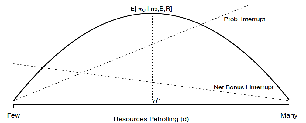
B: Civilian Choices

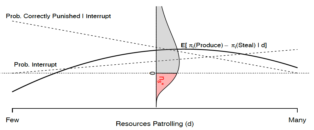
All parameters held constant: $B = 10$ , $R = 10$ , and $[n, \underline{\gamma}, \bar{\gamma}, e, \Omega, \Lambda, s, \psi, \kappa]= [1001,0,2000,620,78,100,1000,160000,1]$

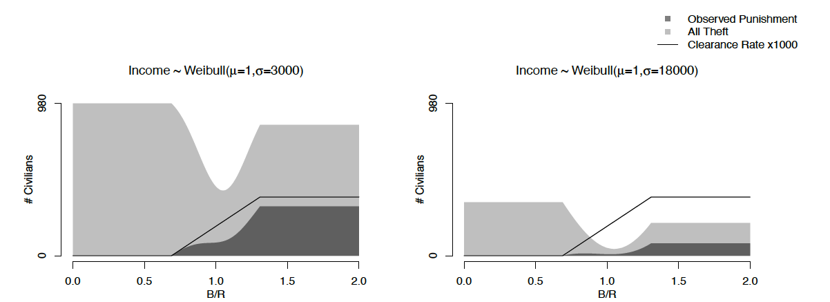
For moderate incentives, crime is minimized at $B/R^{\bullet} = 1 + \frac{s}{\psi \kappa}$ .¹⁶ Figure 2 (crime) provides examples of how the number of thieves changes with $B/R$ . We assume incomes are drawn from a Weibull distribution since this is a good approximation for many income distributions (Bandourian, McDonald, and Turley 2002). The shape parameter is fixed at $\mu=1$ , but the scale parameter is varied: $\sigma \in \{3000, 18000\}$ .

Figure 2 (crime). Incentives × Inequality and the Number of Thieves

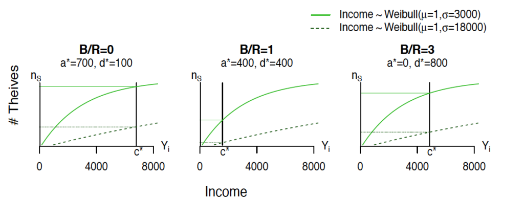
Incomes for 1001 civilian are plotted against their index; the solid light-green line corresponds to incomes from the low-inequality income distribution, and the dashed dark-green line corresponds to incomes from the high-inequality income distribution. Each panel represents a different incentive scheme for the officer, and shows how tokens are allocated to investigation, $a$ , or patrolling, $d$ . In the first panel, where $B / R=0$ , more civilians steal when there is low inequality (as more incomes fall below the cutoff $c$ ). In the second panel, when $B / R=.9$ , the officer allocates more tokens to patrolling, which lowers the cutoff $c$ (due to more effective deterrence in this instance). This causes fewer civilians to steal under the low-inequality distribution, and an even larger reduction under the high-inequality distribution. In the third panel, when $B / R=3$ , the officer allocates even more tokens to patrolling, which increases the cutoff $c$ (due to less effective deterrence), so that more civilians steal. In all panels, parameters are $[\underline{\gamma}, \bar{\gamma}, e, \Omega, \Lambda, s, \psi, \kappa]=[0,700,800,80,100,10000,40000,1]$ .

Notice the efficacy of police incentives depends on the dispersion incomes affects the (as in equation 6). Re-arranging the Figures so that $Y_{i}$ is on y-axis and $n-n_{S}$ is on the x-axis generates a “supply-of-crime” curve. Thus, income inequality (dispersion) changes both the crime level and the crime elasticity with respect to policing parameters.

Figure 3 demonstrates how both the crime rate and the clearance rate change with the incentive scheme. As $B/R$ increases, the officer patrols more, which leads to more interruptions when there is not an offsetting change in the number of thieves. Because there will be changes in the civilian population, the relationship between the incentive scheme and the clearance rate may give the “wrong sign” regarding how police incentives affect crime. The figures show there is a large negative correlation across the 3001 different cases. However, the correlation changes in different environments (e.g., the left panel has a stronger correlation than the right) and in different samples (e.g., the correlation is positive for $B/R \in[1.0,1.25]$ ). Thus, the observed statistics may even paint a misleading \textit{qualitative} picture. Moreover, adding more data (e.g., considering ten times more cases in Figure 3) does not decrease the measurement error. Although one should account for the officer’s incentives in observational data, the complex relationship suggests no clear way to do this.

Figure 3 (measurement). Incentives × Inequality and the Clearance Rate

We consider 3001 cases for $B / R$ equally spaced over the interval [0,2], with other parameters $[\underline{\gamma}, \bar{\gamma}, e, \Omega, \Lambda, s, \psi, \kappa]=[0,2000,620,78,100,8000,160000,1]$ . Each case considers $n=1001$ individuals with incomes spanning a particular Weibull distribution; $Y_i=F_Y^{-1}\left(q_i, \mu, \sigma\right)$ for $q_i \in\{0.05, \ldots 0.95\}$ .

Unfortunately, the ratio of false positives to false negatives does not provide a simple fix to these measurement issues, and has its own set of problems. Figure 4 (justice) shows there is a complex relationship between how both $B/R$ and $F_{Y}$ affect the levels of both types of errors, as well as their ratio. The incentive scheme can have non-monotone effects on error probabilities because the incentives affect two interacting probabilities, that of catching the thief and that of punishing the culprit. When $B/R$ is high, the officer investigates less, which often leads to fewer thieves and more producers being punished—but doesn’t have to if there are large simultaneous changes in the number of thieves. Moreover, Figure 4 shows the falsehood ratio is not necessarily an appropriate summary statistic to focus on because it discards information about the frequency of errors. Many different ratio’s (some increasing in $B/R$ , some decreasing) will reduce both types of error. There are no errors of any type when there is no crime.

Figure 4 (justice). Incentives × Inequality and the Falsehood Ratio

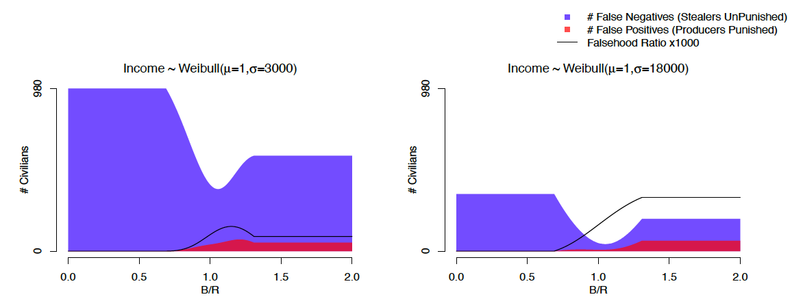
We consider 3001 cases for $B / R$ equally spaced over the interval [0,2]. with other parameters $[\gamma, \bar{\gamma}, e, \Omega, \Lambda, s, \psi, \kappa]=[0,2000,620,78,100,8000,160000,1]$ . Each case considers $n=1001$ individuals with incomes spanning a particular Weibull distribution; $Y_i=F_Y^{-1}\left(q_i, \mu, \sigma\right)$ for $q_i \in\{0.05, \ldots 0.95\}$ .

Together, Figures 3 (measurement) and 4 (justice) also show that when police accountability dramatically improves deterrence (i.e., as $B/R$ goes from 1.25 to 1), it reduces both the level of crime and the rate of false convictions. This reinforces the idea that there is not necessarily a trade-off between false convictions and deterrence.

6 Concluding Discussion

In future work, a more detailed investigation of heterogeneity in theft magnitudes across civilians, as well as heterogeneity in policing bonuses across civilians will be considered.

While many researchers are focused on how to get the right people (e.g., training regimes and selection processes that weed out biased or violent officers), we examine the incentives under which even the right people do the wrong thing. We provide an irreducible truth table of criminal justice that helps understand the multidimensional effects of different incentives, and the corresponding insights may help avoid bad policy.

Our framework provides a dispassionate way to evaluate the complex effects of different policies, without perverse repercussions. A rough estimate as to what would change in our truth table (where we are, and what would change) may prove more helpful than a great estimate of how the clearance-rate changed in any specific town in any specific year. We agree that data is an important component of policy debates, and that a precise understanding of particular mechanisms is important. However, policy should be guided by a deep understanding of all relevant economic forces, and the corresponding equilibrium behavior. Our framework is directly relevant to several recent policy proposals, including numerous calls to increase police accountability.

Policing policy is under scrutiny and several proposed policies increase officer liabilities. Federal legislation, for example, has been recently introduced to end qualified immunity for officers. Opponents of such reforms argue that this would lead to a reduction in police aggressiveness in combating crime, which would cause an increase in crime.¹⁷ In our model, such scrutiny would increase the probability that false convictions are brought to light and curb police malfeasance via an increase in the expected reprimand, R. Whether this will increase or decrease either crime or false positives depends on several factors, including current performance-bonuses, B, as well as several policing and civilian parameters. We show that this “de-policing” hypothesis has theoretical support for some cases. Crucially, we also demonstrate how low police accountability can lead to a high level of false convictions, undermining deterrence and leading to relatively high crime rates. Our model provides two general predictions:

Crime: When B/R is already moderate, either a large decrease or increase in R will cause crime to increase.

Measurement and Justice: When crime is increasing as R decreases, a further decrease in R will cause the clearance rate to increase but also both false positives and crime to increase.

In future work, we believe a promising avenue for theorists is to ground the police metrics that empiricists use (tightening the link between theory and evidence). We focused on modeling the tradeoff between investigation and patrolling using a single representative officer, but an important avenue for future work would be to explore principal-agent problems between a police chief and his officers’ potentially malevolent behaviour. Hundreds of studies identify the causal effect of one particular aspect of policing on another, but this leads to policy advice that is incomplete at best. For now, we recommend that empiricists do not ignore our warnings about reductionism in reforming policy and instead incorporate our truth table of criminal justice. A pragmatic use for current policy debates would be to examine how a proposed policy changes each element of our truth table of criminal justice. To simply let the statistics speak would be a third type of error—not included in our table, but perhaps the central takeaway from this paper.

Another promising avenue for future work is to study the effect of civilian heterogeneity across more dimensions than income. What is the effect of allowing theft magnitudes to vary across civilians on the spatial distribution of crime and police presence? What is the effect of accounting for the fact that police may be incentivized to protect some civilians more than others? This paper is a starting point to formally address such questions.

Appendix A

In formulating our model, we interviewed several police officers and reviewed several police manuals and budgetary documents, which are overviewed here. Most police departments in the United States have a chief who allocates resources among multiple divisions. Departments can request budget increases—in which case they use strategies to “Use crime and workload data judiciously,” “Capitalize on sensational crime incidents,” and “Carefully mobilize interest groups” (Coe and Wiesel 2001). Police departments do not directly control the size of their budget, so they must allocate scarce resources to different divisions. While the size of the budget matters, Lee, Eck, and Corsaro (2016) concluded “this line of research has exhausted its utility. Changing policing strategy is likely to have a greater impact on crime than adding more police.”

There is heterogeneity in departmental structure, but the most common division is between patrolling and investigating.¹⁸ Regardless of departmental structure, most resources are spent on personnel (Police Executive Research Forum 2002). Departments and officers have revenue incentives that are tied to specific metrics. Alpert and Moore (1993) said, “For most practical purposes, these include — 1) reported crime rates, 2) overall arrests, 3) clearance rates, 4) response times are the statistics by which police departments throughout the United States are now held accountable.” This is also true in Canada (Maslov 2016), and perhaps many other countries. Many police departments implement both inducements and sanctions—and they might be there for good reason.

A central issue surrounds performance metrics and undesirable behavior (Tiwana, Bass, and Farrell 2015). Sparrow (2015) summarizes that “officials take actions that are illegal, unethical or excessively risky, and they do so not because they are inherently bad people or motivated by personal gain but because they want to help their agency do better or look better and they are often placed under intense pressure from a narrow set of quantitative performance metrics.” While “clearance rates are indicators of investigative effectiveness but oftentimes can be manipulated and subject to measurement error” (Uchida 2014), the larger issue is that police respond to revenue incentives. A few case studies and experiments suggest such incentives have positive effects (Casari and Plott 2003; DeAngelo and McCannon 2017), but most suggest they cause bad outcomes (Benson 1998; Baicker and Jacobson 2007; Preciado and Wilson 2017; Abbink, Ryvkin, and Serra 2018; Makowsky, Stratmann, and Tabarrok 2018; Harvey and Mungan 2019; Acemoglu et al. 2020). For example, Goldstein, Sances, and You (2018) argued that “police departments in cities that collect a greater share of their revenue from fees solve violent and property crimes at significantly lower rates” and the Ferguson Report (2015) recommends that departments “measure and evaluate individual, supervisory, and agency police performance on community engagement, problem-oriented-policing projects, and crime prevention, rather than on arrest and citation productivity.”¹⁹ However, this also has its own set of unintended consequences: “As a rule of thumb, the department gets ten dollars returned for every dollar invested in training” (Orrick 2018). While pay-for-performance has unintended consequences, it may still be “second-best”: preferable to other incentive schemes or no incentive schemes at all. There are current debates about how police incentives in Minneapolis affect civilian deaths.

Today, “police violence is a leading cause of death for young men in the United States” (Edwards, Lee, and Esposito 2019). Moreover, innocent people are sometimes arrested and convicted, which, alongside deterring crime, is a central concern of the criminal justice system. In the United States, some convictions are overturned by an external review board, but exonerated individuals cannot sue judges, prosecutors, or law enforcement personnel—and must instead rely on compensation statutes. However “To date, less than 30 states have adopted compensation statutes. Without this avenue of relief, many unjustly convicted individuals who have had their lives virtually destroyed by their lengthy incarceration are unable to obtain any monetary reimbursement or services.” (Raeder 2014). We examine how different incentive schemes affect the number of crimes and number of false convictions within this institutional environment.

Appendix B

Here we examine a hide and seek game: thieves place tokens on a property to steal and an officer places tokens on a property to stop them. This discoordination game could go by other names (e.g., attack-defend, battleship, anti-matching pennies) but it is structurally a continuous anti-matching game. The officer wants a token interruption (to catch a thief ), while thieves do not want an interruption (i.e., they want to avoid being caught).

Figure A.5. Interrupt Example

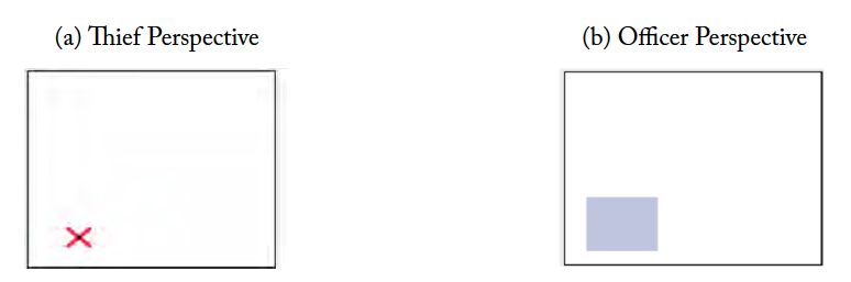
Each steal token is a point with coordinates $(\ell_{i}^{x}, \ell_{i}^{y})$ . Each defend token is a square with width $\Omega$ , that covers $[ \ell_{O}^{x}, \ell_{O}^{y}] \times [\ell_{O}^{x} + {\Omega}, \ell_{O}^{y} + {\Omega}]$ . Both of these reside in the set of properties $\mathbb{P} = \{ \Lambda \times \Lambda \}_{1}^{n}$ , where $n=1$ is represented in Figure A.5. Denote the benefits and costs to $i$ from success and failure as $B^{i}, C^{i}$ , and denote the benefits and costs to $O$ from success and failure as $B^{O}, C^{O}$ . The civilian’s expected profit at a location $\ell_{i}$ , conditional on the officer’s strategy, is

(13) $\begin{eqnarray*} \mathbb{E}[ \Pi_{i}(\ell_{i}) | \sigma_{O} ] = -C_{i} \left[ \int_{\ell_{i}^{y}-\Omega}^{\ell_{i}^{y}} \int_{\ell_{i}^{x}-\Omega}^{\ell_{i}^x} \sigma_{O}(\ell_{O}^{x}, \ell_{O}^{y}) d\ell_{O}^{x} d\ell_{O}^{y} \right] + B_{i}\left[ 1- \int_{\ell_{i}^{y}-\Omega}^{\ell_{i}^{y}} \int_{\ell_{i}^{x}-\Omega}^{\ell_{i}^x} \sigma_{O}(\ell_{O}^{x}, \ell_{O}^{y}) d\ell_{O}^{x} d\ell_{O}^{y} \right] \end{eqnarray*}$

The officer’s expected profit at a location $\ell_{O}$, conditional on the civilian’s strategy, is

(14) $\begin{eqnarray*} \mathbb{E}[ \Pi_{O}(\ell_{O}) | \sigma_{i} ] = B_{O} \left[ \int_{\ell_{O}^{y}}^{\ell_{O}^{y}+\Omega} \int_{\ell_{O}^{x}}^{\ell_{O}^{x}+\Omega} \sigma_{i}(\ell_{i}^{x}, \ell_{i}^{y}) d\ell_{i}^{x} d\ell_{i}^{y} \right] -C_{O} \left[ 1- \int_{\ell_{O}^{y}}^{\ell_{O}^{y}+\Omega} \int_{\ell_{O}^{x}}^{\ell_{O}^{x}+\Omega} \sigma_{i}(\ell_{i}^{x}, \ell_{i}^{y}) d\ell_{i}^{x} d\ell_{i}^{y} \right] \end{eqnarray*}$

Note the bounds for the thief extend to $\ell_{i}-\Omega$ because even when the officer’s lower boundary is at $\ell_{i}-\Omega$ , the token extends up until $\ell_{i}$ . Likewise, the bounds for the officer extend to $\ell_{O}+\Omega$ because even when the officer’s lower boundary is at $\ell_{O}$ , the token extends up until $\ell_{O}+\Omega$ . As discussed in the body, the equilibrium is in mixed strategies.

Proof of Lemma 1 For a single thief and an officer with a single defend token, the equilibrium probability of a defend token interrupting a steal token on a single property is $(\Omega/\Lambda)^2$ .

Because the equilibrium is in mixed strategies, the expected profits are equalized across locations.²⁰ This implies the conditional probabilities of capture are also equalized;

(15) $\begin{eqnarray*} \int_{\ell_{i}^{y}-\Omega}^{\ell_{i}^{y}} \int_{\ell_{i}^{x}-\Omega}^{\ell_{i}^x} \sigma_{O}(\ell_{O}^{x}, \ell_{O}^{y}) d\ell_{O}^{x} d\ell_{O}^{y} &=& \int_{\ell_{i}^{y'}-\Omega}^{\ell_{i}^{y'}} \int_{\ell_{i}^{x'}-\Omega}^{\ell_{i}^{x'}} \sigma_{O}(\ell_{O}^{x}, \ell_{O}^{y}) d\ell_{O}^{x} d\ell_{O}^{y}, \\ \label{eqn:mixedi} \int_{\ell_{O}^{y}}^{\ell_{O}^{y}+\Omega} \int_{\ell_{O}^{x}}^{\ell_{O}^{x}+\Omega} \sigma_{i}(\ell_{i}^{x}, \ell_{i}^{y}) d\ell_{i}^{x} d\ell_{i}^{y} &=& \int_{\ell_{O}^{y'}}^{\ell_{O}^{y'}+\Omega} \int_{\ell_{O}^{x'}}^{\ell_{O}^{x'}+\Omega} \sigma_{i}(\ell_{i}^{x}, \ell_{i}^{y}) d\ell_{i}^{x} d\ell_{i}^{y} \end{eqnarray*}$

To equalize payoffs, the total area covered by the officer token, $\Omega^2$ , is spread evenly over the property area, $\Lambda^2$ . Specifically, the probability of capture conditional on the civilian’s location is

(16) $\begin{eqnarray*} \int_{\ell_{i}^{y}-\Omega}^{\ell_{i}^{y}} \int_{\ell_{i}^{x}-\Omega}^{\ell_{i}^{x}} \sigma_{O}(\ell_{O}^{x}, \ell_{O}^{y}) d\ell_{O}^{x} d\ell_{O}^{y} &=& [\Omega/\Lambda]^2. \end{eqnarray*}$

Then, note that by property of mixed strategies, $\int_{0}^{\Lambda} \int_{0}^{\Lambda} \sigma_{i}(\ell_{i}^{x}, \ell_{i}^{y}) d\ell_{i}^{x} d\ell_{i}^{y} = 1.$ Together, with equation 16, the unconditional probability of an interruption (i.e., the probability of capture conditional on the civilian’s location weighted by the frequency the civilian goes to each location) is

(17) $\begin{eqnarray*} & & \int_{0}^{\Lambda} \int_{0}^{\Lambda} \left[ \int_{\ell_{i}^{y}-\Omega}^{\ell_{i}^{y}} \int_{\ell_{i}^{x}-\Omega}^{\ell_{i}^{x}} \sigma_{O}(\ell_{O}^{x}, \ell_{O}^{y}) d\ell_{O}^{x} d\ell_{O}^{y} \right] \sigma_{i}(\ell_{i}^{x}, \ell_{i}^{y}) d\ell_{i}^{x} d\ell_{i}^{y} \nonumber \\ &=& \left[ \int_{\ell_{i}^{y}-\Omega}^{\ell_{i}^{y}} \int_{\ell_{i}^{x}-\Omega}^{\ell_{i}^{x}} \sigma_{O}(\ell_{O}^{x}, \ell_{O}^{y}) d\ell_{O}^{x} d\ell_{O}^{y} \right] \int_{0}^{\Lambda} \int_{0}^{\Lambda} \sigma_{i}(\ell_{i}^{x}, \ell_{i}^{y}) d\ell_{i}^{x} d\ell_{i}^{y} \nonumber \\ &=& [\Omega/\Lambda]^2 \end{eqnarray*}$

Proof of Lemma 2 For $n_{S}$ thieves and an officer with a single defend token, the equilibrium expected number of interruptions between the steal token and the defend token is $\phi=(\Omega/\Lambda)^2 n_{S}/n$ .

Denote $\sigma_{O}^{j}$ as the share of the tokens the officer spends patrolling property $j$ and $\sigma_{j}^{i}$ as the frequency $j$ steals from $i$ . For a single thief, $i$ , and an officer with a single defend token, the thief steals from only the other $n-1$ civilians. The thief and the officer equalize their mass across the other properties.

(18) $\begin{eqnarray*} \sigma_{0}^{j} &=& \mathbf{1}(j\neq i)/(n-1), \nonumber \\ \sigma_{i}^{j} &=& \mathbf{1}(j\neq i)/(n-1). \end{eqnarray*}$

If the officer is equally uncertain about who the one thief is (subjectively evaluates that each civilian $i$ is thief with probability $1/n$ ), then $\sigma_{0}^{j}=1/n$ .

When there is more than one thief, they steal from n potential civilian properties. The officer mixes evenly across all properties, as do the thieves as a whole (although no thief has mass on his own property). When there are multiple thieves, there are multiple strategies consistent with equilibrium behavior.

(19) $\begin{eqnarray*} \sigma_{0}^{j} &=& 1/n , \nonumber \\ \sum_{i} \sigma_{i}^{j} &=& n_{S}/n. \end{eqnarray*}$

Note that the total expected number of interruptions is $\sum_{j} \left( \Omega/\Lambda \right)^2 \left(\sigma_{O}^{j} \sum_{i} \sigma_{i}^{j} \right) = \left(\Omega/\Lambda\right)^2 n_{S}/n$ except for when $n_{S}=1$ and the officer knows the thief’s identity. However, even in that case, when $n$ is large, $1/(n-1) \approx 1/n$ . Thus, the expected number of interruptions across all properties is

(20) $\begin{eqnarray*} \phi &=& \left(\Omega/\Lambda\right)^2 n_{S}/n. \end{eqnarray*}$

Interestingly, with two thieves and one producer, neither thief has mass on their property, but each has enough mass on the other to equalize payoffs across properties—each poor person more often steals from the other poor person.

Appendix C

Now consider the case in which the bonus the officer obtains depends on the property defended, and the amount a civilian is able to steal depends on the property attacked. From Section B, recall that $B_O^j$ denotes the bonus to an officer from successfully interrupting theft on civilian $j$ ‘s property. Also recall that $B_i^j$ denotes the amount civilian $i$ gets after successfully stealing from civilian $j$ . For simplicity, assume that $\Omega=\Lambda$ (results are robust to relaxing this assumption).

Proposition 9 (Indirect Profits). The officer and a thief expects to earn

(21) $\begin{eqnarray*} \Pi_{O}^{*} &=& \frac{n_{S}}{n} \frac{d }{ 1/n \sum_{j}[B_{O}^{i}]^{-1} } \\ \Pi_{i}^{*} &=& \left[\sum_{j} \frac{B_{i}^{j}}{B_{i}^{j}+C_{i}^{j}} - d \right] \left[ \sum_{j} \frac{1}{B_{i}^{j}+C_{i}^{j}} \right]^{-1} . \end{eqnarray*}$

Proof. The officer chooses the frequency $d$ tokens are allocated to defend each property, $d_{i}= d \sigma_{O}^{i}$ . Given the mixed strategies of thieves, $P^{i}=\sum_{j} \sigma_{j}^{i}$ , the officers’ expected profit at each property is the net reward times the probability of interruption; $B_{O}^{i} \left[ d^{i} P^{i} \right]$ . For the officer to have mixed-strategy optimum; thieves must mix so that $B_{O}^{i} P^{i} = B_{O}^{j} P^{j}$ at properties $i,j$ . Notice that the total mass of thieves is $n_{S}=\sum_{j} P^{j}= \sum_{j} \frac{P^{i} B_{O}^{i}}{ B_{O}^{j}}$ , which implies

(22) $\begin{eqnarray*} P^{i,*} = \frac{n_{S}}{n} \frac{ [B_{O}^{i}]^{-1}}{ 1/n \sum_{j}[B_{O}^{i}]^{-1} }. \end{eqnarray*}$

The officers expected profit is thus

(23) $\begin{eqnarray*} \Pi_{O}=\sum_{j} P^{j} B_{O}^{j} d^{j} = P^{i,*} B_{O}^{i} d = \frac{n_{S}}{n} \frac{d }{ 1/n \sum_{j}[B_{O}^{i}]^{-1} } \end{eqnarray*}$

Similarly, an individual thief $i$ expects to earn $B_{i}^{j} [1-d^{j}] - C_{i}^{j} [d^{j}]$ when stealing from $j$ . For a thief to be indifferent across properties $i,j$ , the officer chooses $d^{j}= \frac{[B_{i}^{j} - B_{i}^{j'} ] + d^{j'} [B_{i}^{j'} + C_{i}^{j'} ]}{B_{i}^{j} + C_{i}^{j}}$ . Notice that the total mass of officer tokens is $d=\sum_{i} d^{i}$ , which implies

(24) $\begin{eqnarray*} d^{j} = \frac{(d-\theta)\gamma + B_{i}^{j}}{B_{i}^{j}+C_{i}^{j}}, \end{eqnarray*}$

where $\theta = \sum_{j} \frac{B_{i}^{j}}{B_{i}^{j}+C_{i}^{j}}$ and $\gamma= \left[ \sum_{j} \frac{1}{B_{i}^{j}+C_{i}^{j}} \right]^{-1}$ . The thieves expected profit is thus

(25) $\begin{eqnarray*} \Pi_{i} = \left[\theta - d \right] \gamma . \end{eqnarray*}$

Remark. In the baseline model, the officer earns $B_{O}^{I}=[B-R][n-2]\rho_{I} + B\rho_{C}$ at each property, which implies $P^{i}= n_{S}/n$ and $\Pi_{O}= \left[d~ n_{S}/n \right] \left[ [B-R][n-2]\rho_{I} + B\rho_{C}\right]$ . Also in the baseline model, a civilian has costs $C_{i}^{j}=\psi \rho_{C}$ and $B_{i}^{j}=s$ , which implies $d^{i}= d/n$ (i.e., $\sigma_{O}^{i}=1/n$ ) and $\Pi_{i}= s - [s + \psi \rho_{C}] d/n$ . Multiplying $d/n$ by $[\Omega/\Lambda]^2$ , so as to account for the uncertainty of capture on each property, yields the baseline profits for both the officer and civilians (equations 2 and 5).

References

Abbink, K., D. Ryvkin, and D. Serra (2018). Corrupt Police. SSRN Working Paper. doi: http://dx.doi.org/10.2139/ssrn.3244092. In preparation.

Acemoglu, D. et al. (2020). “The Perils of High-Powered Incentives: Evidence from Colombia’s False Positives”. In: American Economic Journal: Economic Policy 12.3, 1–43. doi: 10.1257/pol.20180168.

Alpert, G. and M. H. Moore (1993). “Measuring Police Performance in the New Paradigm of Policing”. In: Performance Measures for the Criminal Justice System. Ed. by J. J. DiIulio. US Department of Justice.

Amodio, F. (2019). “Crime Protection Investment Spillovers: Theory and Evidence from the City of Buenos Aires”. In: Journal of Economic Behavior & Organization 159, 626–649. doi: https://doi.org/10.1016/j.jebo.2017.03.023.

Andreoni, J. (1991). “Reasonable Doubt and the Optimal Magnitude of Fines: Should the Penalty Fit the Crime?” In: The RAND Journal of Economics 22.3, 385–395.

Baicker, K. and M. Jacobson (2007). “Finders keepers: Forfeiture laws, policing incentives, and local budgets”. In: Journal of Public Economics 91.11, 2113–2136. doi: https://doi.org/10.1016/j.jpubeco.2007.03.009.

Bandourian, R., J. McDonald, and R. Turley (2002). A Comparison of Parametric Models of Income Distribution across Countries and over Time. LIS Working Paper Series 305. Luxembourg. doi: http://dx.doi.org/10.2139/ssrn.324900.

Banerjee, A. et al. (2019). The Efficient Deployment of Police Resources: Theory and New Evidence from a Randomized Drunk Driving Crackdown in India. Working Paper 26224. National Bureau of Economic Research. doi: 10.3386/w26224.

Becker, G. S. (1968). “Crime and Punishment: An Economic Approach”. In: Journal of Political Economy 76.2, 169–217. doi: 10.1086/259394.

Becker, G. S. and G. J. Stigler (1974). “Law Enforcement, Malfeasance, and Compensation of Enforcers”. In: Journal of Legal Studies 3.1, 1–18.

Benson, B. (1998). To Serve and Protect: Privatization and Community in Criminal Justice. NYU Press. Blanes i Vidal, J. and T. Kirchmaier (2017). “The Effect of Police Response Time on Crime Clearance Rates”. In: Review of Economic Studies 85.2, 855–891. doi: 10.1093/restud/rdx044.

Blanes i Vidal, J. and G. Mastrobuoni (2019). Police Patrols and Crime. IZA Discussion Paper 11393. In preparation.

Blattman, C. et al. (2017). Place-Based Interventions at Scale: The Direct and Spillover Effects of Policing and City Services on Crime. Working Paper 23941. National Bureau of Economic Research. doi: 10.3386/w23941. In preparation.

Bove, V. and E. Gavrilova (2017). “Police Officer on the Frontline or a Soldier? The Effect of Police Militarization on Crime”. In: American Economic Journal: Economic Policy 9.3, 1–18. doi: 10.1257/pol.20150478.

Braga, A. A. et al. (2019). “Hot spots policing and crime reduction: an update of an ongoing systematic review and meta-analysis”. In: Journal of Experimental Criminology. doi: 10.1007/s11292-019-09372-3.

Casari, M. and C. R. Plott (2003). “Decentralized management of common property resources: experiments with a centuries-old institution”. In: Journal of Economic Behavior & Organization 51.2, 217–247. doi: https://doi.org/10.1016/S0167-2681(02)00098-7.

Chalfin, A. (2015). “Economic Costs of Crime”. In: The Encyclopedia of Crime & Punishment. American Cancer Society, 1–12. doi: 10.1002/9781118519639.wbecpx193.

Cheng, C. and W. Long (2018). “Improving Police Services: Evidence from the French Quarter Task Force”. In: Journal of Public Economics 164, 1–18. doi: https://doi.org/10.1016/j.jpubeco.2018.05.002.

Coe, C. K. and D. L. Wiesel (2001). “Police Budgeting: Winning Strategies”. In: Public Administration Review 61.6, 718–727.

Cook, P. J. (1979). “The clearance rate as a measure of criminal justice system effectiveness”. In: Journal of Public Economics 11.1, 135–142. doi: https://doi.org/10.1016/0047-2727(79)90050-1.

DeAngelo, G. and B. C. McCannon (2016). “Public outcry and police behavior”. In: Journal of Economic Analysis & Policy 16.2, 619–645.— (2017). “Judicial Compensation and Performance”. In: Supreme Court Economic Review 25, 129–147. doi: 10.1086/699661.

Devi, T. and J. Fryer Roland G (2020). Policing the Police: The Impact of ”Pattern-or-Practice” Investigations on Crime. Working Paper 27324. National Bureau of Economic Research. doi: 10.3386/w27324.

Dharmapala, D., N. Garoupa, and R. H. McAdams (2016). “Punitive Police? Agency Costs, Law Enforcement, and Criminal Procedure”. In: The Journal of Legal Studies 45.1, 105–141.

Edwards, F., H. Lee, and M. Esposito (2019). “Risk of being killed by police use of force in the United States by age, race–ethnicity, and sex”. In: Proceedings of the National Academy of Sciences 116.34, 16793–16798. doi: 10.1073/pnas.1821204116.

Ehrlich, I. (1973). “Participation in Illegitimate Activities: A Theoretical and Empirical Investigation”. In: Journal of Political Economy 81.3, 521–565.

Friedman, D. (1999). “Why Not Hang Them All: The Virtues of Inefficient Punishment”. In: Journal of Political Economy 107.S6, S259–S269.

Fryer, R. (2020). “A Response to Steven Durlauf and James Heckman”. In: Journal of Political Economy. doi: 10.1086/710977.

Fu, C. and K. I. Wolpin (2017). “Structural Estimation of a Becker-Ehrlich Equilibrium Model of Crime: Allocating Police Across Cities to Reduce Crime”. In: Review of Economic Studies 85.4, 2097–2138. doi: 10.1093/restud/rdx068.

Galiani, S., I. L. Cruz, and G. Torrens (2018). “Stirring up a Hornets’ Nest: Geographic Distribution of Crime”. In: Journal of Economic Behavior & Organization 152, 17–35. doi: https://doi.org/10.1016/j.jebo.2018.06.005.

Galletta, S. (2017). “Law enforcement, municipal budgets and spillover effects: Evidence from a quasi-experiment in Italy”. In: Journal of Urban Economics 101, 90–105. doi: https://doi.org/10.1016/j.jue.2017.06.005.

Gillen, B., E. Snowberg, and L. Yariv (2019). “Experimenting with Measurement Error: Techniques with Applications to the Caltech Cohort Study”. In: Journal of Political Economy 127.4, 1826–1863. doi: 10.1086/701681.

Glaeser, E. L. and B. Sacerdote (1999). “Why Is There More Crime in Cities?” In: Journal of Political Economy 107.S6, S225–S258. doi: 10.1086/250109.

Goldstein, R., M. W. Sances, and H. Y. You (2018). “Exploitative Revenues, Law Enforcement, and the Quality of Government Service”. In: Urban Affairs Review 0.0, 1078087418791775. doi: 10.1177/1078087418791775.

Gonzalez-Navarro, M. (2013). “Deterrence and Geographical Externalities in Auto Theft”. In: American Economic Journal: Applied Economics 5.4, 92–110. doi: 10.1257/app.5.4.92.

Hart, O., A. Shleifer, and R. W. Vishny (1997). “The Proper Scope of Government: Theory and an Application to Prisons”. In: Quarterly Journal of Economics 112.4, 1127–1161. doi: 10.1162/003355300555448.

Harvey, A. and M. C. Mungan (2019). Policing for Profit: The Political Economy of Law Enforcement. Working Paper 19-16. doi: http://dx.doi.org/10.2139/ssrn.3197705.

Heckman, J. J. and S. N. Durlauf (2020). “Comment on ”An Empirical Analysis of Racial Differences in Police Use of Force” by Roland G. Fryer Jr.” In: Journal of Political Economy, null. doi: 10.1086/710976.

Hoeffler, A. (2017). “What Are the Costs of Violence?” In: Politics, Philosophy & Economics 16.4, 422–445. doi: 10.1177/1470594X17714270.

Holmstrom, B. and P. Milgrom (1987). “Aggregation and Linearity in the Provision of Intertemporal Incentives”. In: Econometrica 55.2, 303–328. — (1991). “Multitask Principal-Agent Analyses: Incentive Contracts, Asset Ownership, and Job Design”. In: Journal of Law, Economics, & Organization 7, 24–52.

Hsieh Ching-Chi Pugh, M. D. (1993). “Poverty, Income Inequality, and Violent Crime: A Meta-Analysis of Recent Aggregate Data Studies”. In: Criminal Justice Review 18, 182.

İmrohoroğlu, A., A. Merlo, and P. Rupert (2000). “On the Political Economy of Income Redistribution and Crime”. In: International Economic Review 41.1, 1–25.

Johnson, S. D., R. T. Guerette, and K. Bowers (2014). “Crime displacement: what we know, what we don’t know, and what it means for crime reduction”. In: Journal of Experimental Criminology 10.4, 549–571. doi: 10.1007/s11292-014-9209-4.

Kaplow, L. and S. Shavell (1994). “Accuracy in the Determination of Liability”. In: The Journal of Law and Economics 37.1, 1–15. doi: 10.1086/467304.

Landes, W. M. and R. A. Posner (1975). “The Private Enforcement of Law”. In: Journal of Legal Studies4.1, 1–46.

Lando, H. and M. C. Mungan (2018). “The effect of type-1 error on deterrence”. In: International Review of Law and Economics 53, 1–8. doi: https://doi.org/10.1016/j.irle.2017.08.001.

Lazzati, N. and A. A. Menichini (2016). “Hot Spot Policing: A Study of Place-Based Strategies for Crime Prevention”. In: Southern Economic Journal 82.3, 893–913. doi: 10.1002/soej.12112.

Lee, Y., J. E. Eck, and N. Corsaro (2016). “Conclusions from the history of research into the effects of police force size on crime – 1968 through 2013: a historical systematic review”. In: Journal of Experimental Criminology 12 (3), 431–451. doi: 10.1007/s11292-016-9269-8.

Levitt, S. D. (1997). “Using Electoral Cycles in Police Hiring to Estimate the Effect of Police on Crime”. In: American Economic Review 87.3, 270–290.

Maheshri, V. and G. Mastrobuoni (2020). “The Race Between Deterrence and Displacement: Theory and Evidence from Bank Robberies”. In: Review of Economics and Statistics 0.ja, 1–45. doi: 10.1162/rest\_a\_00900.

Makowsky, M. D., T. Stratmann, and A. T. Tabarrok (2018). To Serve and Collect: The Fiscal and Racial Determinants of Law Enforcement. Tech. rep. 16-17. doi: http://dx.doi.org/10.2139/ssrn.2745000.

Markussen, T., L. Putterman, and J.-R. Tyran (2016). “Judicial Error and Cooperation”. In: European Economic Review 89, 372–388. doi: https://doi.org/10.1016/j.euroecorev.2016.08.004.

Maslov, A. (2016). Measuring the Performance of the Police: The Perspective of the Public. Research Report 2015–R034.

Mastrobuoni, G. (2019). “Police Disruption and Performance: Evidence from Recurrent Redeployments within a City”. In: Journal of Public Economics 176, 18–31. doi: https://doi.org/10.1016/j.jpubeco.2019.05.003.— (2020). “Crime is Terribly Revealing: Information Technology and Police Productivity”. In: Review of Economic Studies. doi: 10.1093/restud/rdaa009.

Nagin, D., R. Solow, and C. Lum (2015). “Deterrence, Criminal Opportunities, and Police”. In: Criminology 53.1, 74–100.

Novak, K. J. (2014). “Preventive Patrol”. In: Encyclopedia of Criminology and Criminal Justice. Ed. by Bruinsma and D. Weisburd. New York, NY: Springer New York, 3921–3931. doi: 10.1007/978-1-4614-5690-2_269.

Orrick, W. D. (2018). Budgeting in Small Police Agencies. Tech. rep.

Paré, P.-P., R. Felson, and M. Ouimet (2007). “Community Variation in Crime Clearance: A Multilevel Analysis with Comments on Assessing Police Performance”. In: Journal of Quantitative Criminology 23.3, 243–258.

Persson, M. and C.-H. Siven (2007). “The Becker Paradox and Type I Versus Type II Errors in the Economics of Crime”. In: International Economic Review 48.1, 211–233.

Pogarsky, G. and T. Loughran (2016). “The Policy-to-Perceptions Link in Deterrence: Time to Retire the Clearance Rate”. In: Criminology & Public Policy 15.3, 777–790.

Police Executive Research Forum (2002). Police Department Budgeting: A Guide for Law Enforcement Chief Executives. Tech. rep.

Preciado, M. and B. J. Wilson (2017). “The Welfare Effects of Civil Forfeiture”. In: Review of Behavioral Economics 4.2, 153–179. doi: 10.1561/105.00000063.

Pridemore, W. A. (2011). “Poverty Matters: A Reassessment of the Inequality–Homicide Relationship in Cross-National Studies”. In: British Journal of Criminology 51.5, 739–772. doi: 10.1093/bjc/azr019.

Rabin, C., J. Weaver, and D. Ovalle (2018). The chief wanted perfect stats, so cops were told to pin crimes on black people, probe found.

Raeder, M. (2014). “Overturning Wrongful Convictions and Compensating Exonerees”. In: Encyclopedia of Criminology and Criminal Justice. Ed. by G. Bruinsma and D. Weisburd. New York, NY: Springer New York, 3417–3428. doi: 10.1007/978-1-4614-5690-2_163.

Rizzolli, M. and M. Saraceno (2013). “Better that ten guilty persons escape: punishment costs explain the standard of evidence”. In: Public Choice 155.3/4, 395–411.

Rizzolli, M. and L. Stanca (2012). “Judicial Errors and Crime Deterrence: Theory and Experimental Evidence”. In: The Journal of Law and Economics 55.2, 311–338. doi: 10.1086/663346.

Rushin, S. and G. Edwards (2016). “De-policing”. In: Cornell L. Rev. 102, 721.

Shi, L. (2009). “The limit of oversight in policing: Evidence from the 2001 Cincinnati riot”. In: Journal of Public Economics 93.1, 99–113. doi: https://doi.org/10.1016/j.jpubeco.2008.07.007.

Sparrow, M. K. (2015). Measuring Performance in a Modern Police Organization. Tech. rep. Harvard Kennedy School.

Telep, C. W. et al. (2014). “Displacement of crime and diffusion of crime control benefits in large-scale geographic areas: a systematic review”. In: Journal of Experimental Criminology 10.4, 515–548. doi: 10.1007/s11292-014-9208-5.

Tiwana, N., G. Bass, and G. Farrell (2015). “Police performance measurement: an annotated bibliography”. In: Crime Science 4 (1). doi: 10.1186/s40163-014-0011-4.

Tsebelis, G. (1989). “The Abuse of Probability in Political Analysis: The Robinson Crusoe Fallacy”. In: American Political Science Review 83.1, 77–91. doi: 10.2307/1956435.

Uchida, C. D. (2014). “Police Performance Measurement”. In: Encyclopedia of Criminology and Criminal Justice. Ed. by G. Bruinsma and D. Weisburd. New York, NY: Springer New York, 3702–3711. doi: 10.1007/978-1-4614-5690-2_186.

United States Department of Justice, C. R. D. (2015). The Ferguson Report: Department of Justice Investigation of the Ferguson Police Department. New Press.

Volokh, A. (1997). “n Guilty Men”. In: University of Pennsylvania Law Review 146.1, 173–216. Weisburd, S. (2020). “Police Presence, Rapid Response Rates, and Crime Prevention”. In: The Review of Economics and Statistics 0.ja, 1–45. doi: 10.1162/rest\_a\_00889.

How Policing Incentives Affect Crime, Measurement, and Justice

Executive Summary

Resources

Focuses

1 Introduction

3 Theory

3.1 Thieves Hide and Officers Seek

3.2 Officers Patrol and Investigate, Civilians Produce or Steal

4 Insights for Crime, Measurement, and Justice

5 Parametric Examples

6 Concluding Discussion

Appendix A

Appendix B

Appendix C

References

Executive Summary

Resources

Related Publications

Related News

Related Blogs

Focuses

1 Introduction

2 Related Literature

3 Theory

3.1 Thieves Hide and Officers Seek

3.2 Officers Patrol and Investigate, Civilians Produce or Steal

4 Insights for Crime, Measurement, and Justice

5 Parametric Examples

6 Concluding Discussion

Appendix A

Appendix B

Appendix C

References