
1 Introduction
“But marital relationships, parent-child relationships, decisions to marry and divorce, etc., are also profoundly economic acts. Becker blasted through the Victorian detritus of all that bourgeois romantic ideology to analyze the ways in which marital and reproductive behaviors are fundamentally rooted in a utilitarian economic calculus.”
— Kathleen Geier
Gary Becker (1973) famously argued that positive gains from marriage and negative consequences of getting divorced are what motivates two individuals to stay in a marriage. The legal status of marriage itself bestows a wide range of social, economic, and legal benefits for those who choose to participate in a marital contract. Marriage is thus often associated with economic stability and security (Gibson-Davis, Edin, and McLanahan 2005). One of the broad objectives of the Personal Responsibility and Work Opportunity Reconciliation Act (PRWORA) of 1996 was in fact the promotion of marriage, in addition to promoting work and reducing childbirth out of wedlock. Promotion of marriage and a two-parent household was considered to be a means to reduce poverty under welfare reform (Hu 2003). While policies that affect the costs and benefits of marriage can be reasonably expected to affect an individual’s decisions to marry, stay married, or to divorce, a longstanding question of interest to economists is whether economic incentives created by policies can truly affect marital decision.
One benefit of marriage is access to dependent health insurance coverage through one’s spouse. In the United States, around 152 million non-elderly people are covered by employer-provided health insurance, according to the Kaiser Family Foundation (KFF) 2018 Employer Health Benefits Survey, and among these a substantial proportion are covered as dependents. Thus, it is reasonable to consider the prospect of obtaining health insurance coverage to be an important consideration for individuals’ decisions to marry as well to stay in a marriage. While this may not be important for those who have access to health insurance coverage on their own (employer- or government-provided), many individuals are not eligible for these forms of coverage and thus resort to dependent coverage. Low-income childless adults who did not qualify for state-provided coverage such as Medicaid, did not have ESHI (Employer-Sponsored Health Insurance), or could not afford private coverage are people who would especially fit into this vulnerable category. Moreover, dissolution of marriage makes a person vulnerable to the prospect of losing coverage, reiterating the link between health insurance and marital status.
Policies that change the eligibility for different sources of health insurance can alter their relative costs. If such policies provide an alternative source of coverage outside of marriage, or if such policies remove any barriers to marriage that had previously made marriage costly, one can expect them to impact marital decision-making as well. The Affordable Care Act (ACA) aimed to achieve nearly universal health insurance coverage in the United States through a number of major provisions that took effect in 2014, including the expansion of Medicaid. The purpose of this paper is to identify the causal impact of the ACA Medicaid expansion on the propensity to marry and divorce, using data from the American Community Survey and using a difference-in-differences (DD) identification strategy that exploits variation across time and state Medicaid expansion status.
While popular media has reported anecdotal evidence on the association between the ACA and marital decision-making, this paper attempts to causally estimate the impact of the ACA Medicaid expansion on marriage and divorce decisions. By considering divorces, I also try to address the possibility of the incidence of “marriage-lock,” whereby individuals decide to stay married to access dependent coverage through their spouse’s health insurance. Since women (25 percent) are still more likely to be covered as dependents on ESHI policies than men (13 percent), it is important to stratify the analysis by gender (Peters, Simon, and Taber 2014). Thus, this analysis provides a basis to examine whether such economic incentives affect marriage and family structure.
The results indicate that among low-educated (defined as those with a high school diploma or lower), non-elderly adults over 26 years of age (i.e., excluding young adults), the Medicaid expansion results in a statistically significant decrease in the likelihood of being newly married. There is a total reduction of 6.92 percent, which is particularly driven by females, who show a reduction of 11.6 percent in the likelihood of being married. A concurrent paper by Hampton and Lenhart (2019) studying the impact of Medicaid expansion on marital decision-making finds a similar result with reduction in marriage. As the theoretical predictions suggest, a plausible explanation is that Medicaid serves as an alternative source of coverage in place of dependent coverage such that people substitute away from dependent coverage (which would entail marriage when they can attain Medicaid when single). The results for divorces also support this explanation, although they are more associational in nature. However, my results broadly support the narrative that incentives to gain coverage can affect marital decisions and thereby family structure.
2 Background
There is now a substantial body of literature that looks at how health insurance within marriage affects labor market decisions. The effects of ESHI on labor supply of married women has shown that spouses’ coverage negatively affects the number of hours women worked (Buchmueller and Valletta 1999). Wellington and Cobb-Clark (2000) also find that even husbands who receive health insurance coverage through their wives’ employment work fewer hours than husbands who do not, even though the impact is larger for wives covered by their husbands’ insurance. Abraham and Royalty (2005) argue that having a second earner in the household can improve household health insurance options, access, coverage, and generosity, particularly for vulnerable workers (part-time, self-employed, and workers in small firms).
One of the earliest empirical works that attempts to quantify the relationship between marital disruption and loss of health insurance (Zimmer 2007) finds that marital separation immediately increases the rate of insurance loss by approximately 20 percentage points among wives who are dependent on their husbands’ policies. In their seminal work, Lavelle and Smock (2012) find that approximately 115,000 American women lose private health insurance each year immediately after divorce and that slightly more than one-half become uninsured as a result. However, baseline factors are found to moderate loss of coverage after divorce (e.g., factors such as employment status, source of coverage when married, education, job, poverty status, etc.), thus accounting for subgroup heterogeneity in evaluating these results. 1Their estimates are smaller than those provided by Zimmer (2007), primarily because they control for selection bias in the data, which many of the earlier studies, including Zimmer (2007), fail to do. Zimmer fails to account for the baseline disparity whereby even married women who later divorce are more likely to be uninsured than women who remain married. Lavelle and Smock (2012) account for the role of selection in their study, which may arise from the fact that divorced women may be at a more disadvantageous position relative to married women to begin with. Thus, Lavelle and Smock start off by measuring the extent to which married women differ from divorced women on pre-divorce characteristics and rates of health insurance coverage. They then apply a multivariate fixed effects model that controls for time-invariant characteristics, subgroup heterogeneities, and time heterogeneity.
Subsequent work using the Survey of Income and Program Participation (SIPP) data by Peters, Simon, and Taber (2014) extends the analysis to include both divorced and separated to find that individual-based private coverage increases, irrespective of gender, after marriage dissolution.2They use the 1996, 2001, and 2004 panels of the SIPP. However, the decreases in dependent coverage are much larger and offset the increase in private coverage. Children and women show an increase in public coverage around the time of separation or divorce. Sohn (2015) applies a hazard model to married individuals and finds that, on average, people who were covered as dependents through their spouse’s health plans had lower rates of divorce, showing some support for the incidence of “marriage lock.” Moreover, not having an alternative source of health insurance outside their current plan as dependents further diminished risks of divorce or separation.
Healthcare policies, especially those relating to coverage eligibility, can affect marital decisions. Yelowitz (1998) finds that the expansion of Medicaid eligibility in the 1980s and 1990s to include married parent families who were not on Aid to Families with Dependent Children (AFDC) led to an increase in the probability of marriage. Abramowitz (2016) has looked at the impact of the young adult provisions (YAP) of the ACA in 2010 on the probability of marriage given that the YAP opens up a new avenue to access health insurance outside marriage. This paper uses a difference-in-differences analysis and exploits variation across age groups and over time to identify the impact of ACA young adult provision on the likelihood of marriage. The results find a decrease in marriage, cohabitation, and spousal health insurance among the treatment group (individuals aged 23–25 years) and an increase in divorces. Heim, Lurie, and Simon (2018) use administrative panel data on taxes to also study the impact of the ACA YAP on childbearing and marriage. In addition to finding a decline in marriage among individuals aged 24–25, they particularly find reduced childbearing among young women who are unmarried, those with fewer than two prior children, and those not in post-secondary school.
Barkowski and McLaughlin (2020) study the influence of US state and federal health insurance coverage mandates on the marriage of young adults. They find that pre-ACA marriage rates of eligible young adults in states with coverage mandates were lower than ineligible young adults in the same states. This pattern reversed upon the passage of the ACA, with marriage becoming more likely among eligible young adults than ineligible ones. In contrast to Abramowitz (2016), they find that the effect of the ACA on marriage was not uniformly negative, with the complete picture of how the law changed marital behavior depending on the interaction of both the federal and state mandates. Chen (2019) also studies marriage and divorce decisions caused by the introduction of the Massachusetts healthcare reforms of 2006 using the data from ACS and finds a reduction in divorce rates and an increase in marriage rates.
Among studies regarding the impact of Medicaid expansion on marital decision, Slusky and Ginther (2017) examine the ACA Medicaid expansions and find that they led to a decrease in medical divorce for college-educated individuals between the ages of 50 and 64. The closest paper to this study that also studies Medicaid expansion and marital decisions is by Hampton and Lenhart (2019) using the Current Population Survey. However, that paper uses marital status as the dependent variable at the time of the survey and not entry into new marriages. As a result Hampton and Lenhart study the stock of marriages rather than flows into and out of marriages as a result of the Medicaid expansion. Their paper also includes young adults in the sample—those affected by the young adult provisions of the ACA—and can lead to a confound with the sole impact of the ACA Medicaid expansion. However, this paper too finds a reduction in the likelihood of marriage and an increase in the likelihood of divorce.
3 Theoretical Framework
The goal of the Patient Protection and Affordable Care Act (ACA) of March 2010 was to achieve nearly universal health insurance coverage in the United States through a “three-legged stool approach” involving a combination of insurance market reforms, mandates, subsidies, health insurance exchanges, and Medicaid expansions (Gruber 2011). The major components of the ACA took effect in 2014, and these provisions were especially important for low-income individuals, women, and childless adults. The three-legged stool approach addressed the affordability of individual mandates by subsidies and Medicaid expansion. In this section, I discuss how the Medicaid expansion may affect decisions to marry or divorce through a stylized model of marital decision-making.
Previously, Medicaid eligibility was typically tied to those with low income among specific groups such as children, pregnant women, elderly and disabled individuals, and some parents, but excluded other low-income adults. With the ACA Medicaid expansion, Medicaid eligibility was no longer categorical. In Medicaid expansion states, Medicaid was made available up to 138 percent of the federal poverty level (FPL). Since the Supreme Court verdict in 2012 allowed states to opt out of the requirement to expand Medicaid, Medicaid eligibility in non-expansion states still remained limited by category, with childless adults remaining ineligible in most states and only some parents being eligible. For example, in a KFF survey Brooks et al. (2019) report that for non-expansion states, the median eligibility limit for parents was 40 percent of FPL which was about $8,532 for a family of three as of 2019.
It is important to understand the possible theoretical channels through which the ACA Medicaid expansion can impact marital decisions. With respect to health insurance coverage that is relevant to the research question, two primary impacts of the Medicaid expansion would be a reduction of the cost of coverage and an improvement in access to coverage (through changes in eligibility). These can alter the relative costs of different sources of insurance and thereby the relative benefits and costs of marriage initiation or termination. It is important to note here that my question is essentially a cross-sectional question that aims to study how expanding the generosity of the Medicaid program impacts transition in and out of marriage.
I model the decision to marry or remain married to understand how having health insurance coverage through the Medicaid expansion affects marital decision-making among low-income individuals below 138 percent of FPL. The model is based on the theory of marriage by Becker (1973, 1981) and subsequent adaptation by Chen (2018). The central idea of this model is that people enter into marriages or remain in marriages if the expected utility derived from being single is lower than that of being in a marital union.
Consider a model of marital decision-making with agents who seek each other in the marriage market, with strictly quasi-linear preferences as follows:
(1) 
where M denotes the state of being married and S denotes the state of being single (or divorced). V denotes the utility gain (measured in dollar units) from marriage (such as having children, income, companionship, love, security, etc.), and H is the utility (measured in dollar units) derived from having health insurance coverage.  is the premium or cost of health insurance. I assume that the utility from health insurance is the same across the state of being married or single.
I make the following simplifying assumptions. First, I assume that individuals always have health insurance of some form, since having coverage is strictly preferred to not having coverage. Second, I assume that the utility derived from health insurance is identical across all plans. Third, I assume that without Medicaid expansion, low-income individuals either had only ESHI (employer-sponsored health insurance) through spouses if married, or non-group insurance if single. ACA Medicaid expansion expanded eligibility for Medicaid such that single low-income individuals now qualified for Medicaid. Moreover, households with income below 138 percent of FPL also qualified for Medicaid after the expansion. Recall that, previously, Medicaid eligibility was quite limited in that it covered low-income children, pregnant women, elderly and disabled individuals, and some parents, but excluded other low-income adults. Fourth, I analyze the decisions of low-income individuals only (<138 percent of FPL), as Medicaid expansion is likely to affect them. Thus, we have the following:
(2) 
(3) 
(4) 
An individual decides whether to enter or leave a marriage. In order to do this they undertake the following optimization:
(5) ![\begin{equation*} Max[U_M - U_S, 0]. \end{equation*}](https://www.thecgo.org/wp-content/ql-cache/quicklatex.com-7fa39a5b643937ef351ecc7ec85c2528_l3.svg "Rendered by QuickLaTeX.com")
Substituting (2) and (3) in (5), we have
(6) 
Now I assume that for the marginal agent, the utility is equal across two states (i.e., $U_S = U_M$). Now this implies from (6) that
(7) 
(8) 
Thus for the marginal agent, the net benefit from being married is the same as the net benefit from being single.
Consider an agent who prefers being single to being married without consideration of health insurance. Thus we have  . Without Medicaid, we know
  . Therefore, individuals for whom the premium of non-group insurance far outweighs the benefits of being single (i.e.,
  ) such that the net benefit from staying single is lower than the net benefit of being married, will choose to marry or stay married.
Following Medicaid expansion, we know that  , since
  . As a result, the net benefit from being single will now outweigh the net benefit of being married for more people. This is because, given , as
  falls such that it is lower than
  , we have
  . Thus, the net benefit from staying single outweighs the net benefit from marriage for more people. Therefore, we can expect new marriages to decrease, since fewer people (who would choose to remain single without accounting for health insurance) can be induced to marry or stay married now.
As a result, the hypothesis is that Medicaid expansion will lead to a drop in new marriages among individuals within the low-income population who are likely to be affected by Medicaid expansion and would have otherwise preferred to be single.
4 Data and Method
This section describes the choice of the sample for my analysis and the methodology implemented for identifying the impact of the ACA Medicaid expansion on marital decision-making.
4.1 Data and Sample Selection
The primary data source is the American Community Survey (ACS), a nationwide survey administered by the Census Bureau asking detailed questions about population and housing characteristics. The ACS is well suited for this study since it has variables that allow for the measures of marriage initiation and termination (not just the stock of marriage or divorces). The dependent variable for marriage initiation captures all those who are newly married. Defined specifically, the dependent variable is “whether an individual got married in the calendar year prior to the survey year” constructed from the ”year last married” variable from ACS. This is same as the measure used by Abramowitz (2016) in evaluating the impact of the young adult provision of the ACA on marriage. It does not look at the stock of married people in the sample, since that would reflect both current and past conditions, but instead concentrates on those who initiated marriage recently. For divorces, there is no similarly defined variable as “year last married.” So instead I use the variable measuring whether individuals got divorced in the last 12 months as an indicator for newly divorced. 3A similar variable for marriage asks whether a person was married in the past 12 months, for which data are also available in the ACS. A drawback to using this variable is that, given that the ACS is conducted throughout the year, it is not possible to clearly identify individuals’ dates of marriage precisely enough to identify whether they married during the pre-treatment or post-treatment period using the publicly available ACS data. However, I use this variable as a robustness check.
The main sample for studying marriage initiation includes low-educated (high school diploma or less) adults between the ages of 27 and 64 who got married or remained unmarried in a calendar year previous to the survey year. For divorces, the sample includes low-educated (high school diploma or less) adults between the ages of 27 and 64 who got divorced in the past 12 months and all those who remained married, for each calendar year. Recall that the Medicaid expansion is targeted at low-income individuals. Following Kaestner et al. (2015), I limit the sample to low-educated individuals as a proxy for low income, since education and income are strongly correlated and selecting a sample based on income can lead to biases, as Medicaid can affect both marital decisions and income. Young adults ages 18 to26 are removed from the sample as they may be affected by the young adult provision of the ACA.
I consider the time period consisting of ACS survey years 2011 to 2017. Since the outcome variable is lagged, I use the survey years 2011 to 2014 as the pre-treatment period, which captures new marriages between 2010 and 2013. The post-treatment period includes survey years 2015 to 2017, which capture new marriages between 2014 to 2016 calendar years. The categorization of the expansion states is done in accordance with KFF and Centers for Medicare and Medicaid Services (CMS), which put the number of states that expanded Medicaid by December 2017 at 31 states and Washington DC (AK, AZ, AR, CA, CO, CT, DE, DC, HI, IL, IN, IA, KY, LA MD, MA, MI, MN, MT, NH, NJ, NY, ND, NM, NV, OH, OR, PA, RI, VT, WA, and WV). Since the ACA allowed states the option to extend their eligibility prior to 2014, my results should be interpreted as pertaining only to the effects from states that expanded Medicaid between January 2014 and December 2017, and may be underestimating the effect of the total expansion from 2010 to 2017.4In robustness checks discussed later, I will consider early expanders and the degree of expansion among these early expanders to mitigate potential confounds in the results arising from early expanders.
Table 1 presents the summary statistics for the sample of new marriages used in my analysis (i.e., all non-elderly adults above the age of 26, with a high school diploma or less, who got married or remained unmarried in the calendar year prior to the survey year). Expansion states show a slight increase in the proportion of new marriages post expansion, although the difference is not significant. Non-expansion states show an increase in marriages in the post-expansion period, and the difference is significant at the 1 percent level. Thus there seems to be a relative reduction in the proportion married in expansion states compared to non-expansion states, post expansion. There are some differences in the demographic characteristics of the expansion and non-expansion states that I control for in the regression analysis.
Table 1. Summary Statistics
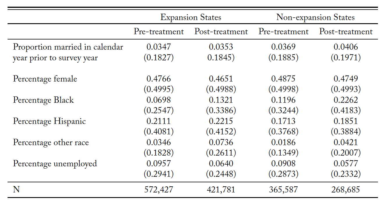
Source: American Community Survey 1-year estimates. Survey years 2011 to 2017.
4.2 Identification Strategy
My identification strategy addresses the Medicaid expansion of the ACA and its impact on marital decisions by exploiting the variation in time and state Medicaid expansion status as in Simon, Soni, and Cawley (2017). Thus I compare changes in outcomes in the treatment states to the same outcomes in the control states.
The treatment states are the ones that expanded Medicaid to low-income adults between January 2014 and December 2017. The control consists of the rest of the states, which had not yet expanded Medicaid to this population. Formally, I estimate the following difference-in-differences (DiD) regression:
(9) 
 is the binary marriage outcome for individual
  in state
  in year
  ,
,  is an indicator for whether period
  is in the post-treatment period, and
  is an indicator for whether state
  expanded Medicaid.
  is a vector of control variables that includes demographic characteristics (such as gender, age, race, citizenship, education, and whether person is foreign-born), family characteristics (such as number of children and household income), unemployment status, and seasonally adjusted monthly state unemployment rate from the Bureau of Labor Statistics.
  and
and  are state and time fixed effects, respectively. The outcome variable of interest is binary in whether an individual was newly married or newly divorced, based on the definitions given earlier. I estimate a linear probability model for our binary dependent variable of interest since this type of model is typically known to give reliable estimates of average effects (Angrist and Pischke 2008). Standard errors are clustered by states.
The identifying assumption of the DD model is that the outcomes would follow similar trends in Medicaid expansion and non-expansion states in the absence of the ACA, conditional on the covariates. Given that this assumption holds, the coefficient  identifies the impact of Medicaid expansion on the outcome.
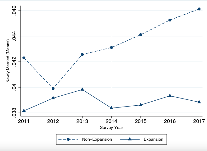
A state’s Medicaid expansion decision is highly political in nature, with predominantly Republican states less likely to undertake Medicaid expansions. I test this assumption first informally by graphically comparing the trends. Figures 1, 2, and 3 provide the trends in the proportion of newly married in the sample across treatment and control groups separately. Visually inspecting trends leading up to treatment between control and treated states can, perhaps, engender confidence in the key identifying assumption, even if not a formal test. Thus I assume that in the absence of the intervention (i.e., the Medicaid expansion), we would expect to see similar trends in the expansion and non-expansion states. In addition to this, I test the common trend assumption more formally by carrying out an event study analysis. The event study is discussed under the robustness checks.
Figure 1. Trends for Newly Married: Full Sample
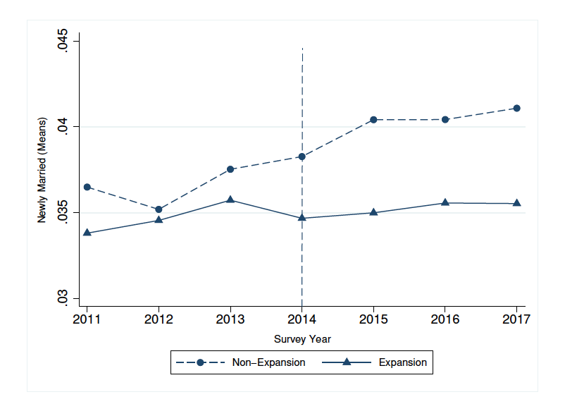
Figure 2. Trends for Newly Married: Females
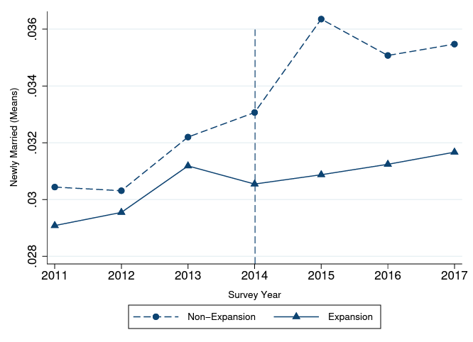
Figure 3. Trends for Newly Married: Males
5 Results
This section discusses the main results of the two outcomes of interest: new marriages and new divorces obtained from the DD specification. Additionally, robustness checks and sensitivity analyses are also reported.
5.1 Results for Marriage
This section summarizes the impact of the Medicaid expansion on the decision to marry as estimated by the DD model. Table 2 presents the results of the baseline DD model. Column 1 presents results for the entire sample, while columns 2 and 3 present the results for females and males, respectively. I employ a wild cluster bootstrap resampling method as proposed by Cameron, Gelbach, and Miller (2008) to account for the fact that the small number of clusters may lead to the over-rejection of the null.
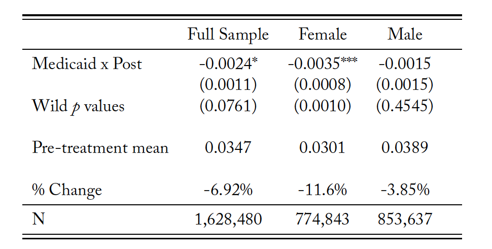
Table 2. Newly Married Difference-in-Differences Estimates
Source: American Community Survey.
Notes: The sample is restricted to non-elderly adults above 26 years of age with a high school diploma or less, who got married or stayed unmarried in the calendar year previous to the survey year. Regression includes demographic, family, income, and unemployment controls. P values using wild bootstrap clustering method are reported. The symbol *** indicates significance at the 1 percent level, ** is significant at the 2 percent level, and * is significant at the 10 percent level.
It should be mentioned here that I carry out an event study analysis to check for comment trends. The parallel pre-trends suggest that the common trends assumption is likely to hold. Thus the results for marriages may be interpreted causally. I discuss the event study analysis in detail later. The results show that the expansion of Medicaid eligibility reduced the propensity to marry significantly. In the full sample, the probability of being newly married decreased by 0.2 percentage points, which represents a 6.9 percent decrease in marriage rates among low-educated, non-elderly adults above 26 years of age, compared to before Medicaid expansion.
While there is an overall negative effect of Medicaid expansion on the propensity to marry, the provision may have a differential impact on different subsections of the population. For example men and women may have differential access to health insurance or varying degrees of dependence on spousal coverage. Therefore, I first stratify the sample by sex and find that Medicaid expansion reduces the propensity to marry among both men and women. I find that expansion in Medicaid eligibility leads to a decrease of 0.35 percentage points (i.e., an 11.6 percent drop) in new marriages in the subsample of women relative to their pre-treatment mean. The reduction for men is 0.15 percentage points (or 3.9 percent) from their pre-treatment mean and is not statistically significant. However, the estimates for men and women are not statistically significantly different from each other. Thus there is no heterogeneous effect by sex on the propensity of being newly married due to Medicaid expansion (p=0.14).
The studies on the young adult provision of the ACA and its impact on marriage show a similar substitution away from marriage. Both Abramowitz (2016) and Heim, Lurie, and Simon (2018) find a 0.5 percentage point reduction among those between the ages of 23 and 25, which is a 9.3 and 2.1 percent reduction in the respective samples of these studies. Hampton and Lenhart (2019) find a 2.13 percent reduction in the likelihood of being married.
Thus the results support the theoretically plausible explanation that in the presence of an alternate source of coverage, individuals substitute away from dependent coverage through marriage, thereby showing a reduction in the propensity to marry. As discussed in the theoretical section, incentives that can cause individuals to substitute away from marriage as a source of health insurance coverage can also affect other marital outcomes, such as divorce. An alternate source of coverage can also reduce the cost of divorce.
5.2 Results for Divorces
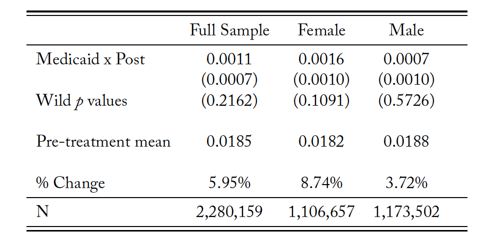
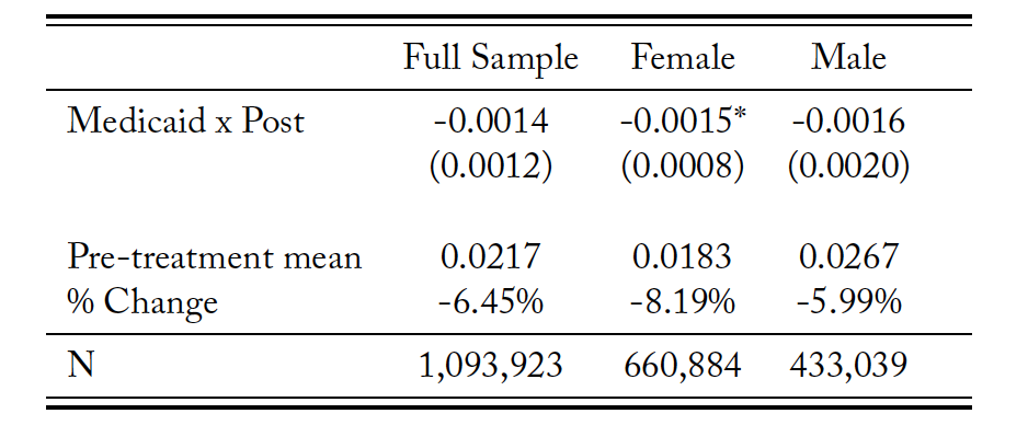
Table 3 presents the results of new divorces. The results indicate that the Medicaid expansion is associated with an increase in the likelihood of having divorced in the past 12 months. Although statistically insignificant, there is an increase in divorces in the sample by 0.11 percentage points, or 5.95 percent. The subsample for women shows an increase of 0.16 percentage points, or 8.74 percent. Men show a 0.07 percentage point increase in the likelihood of new divorces. However, there is no heterogeneous effect on the likelihood of divorces by sex, as the estimates are not statistically significantly different from each other (p=0.42).
However, these results are associational in nature since the common trends assumption does not hold for divorces given our model. In the event study presented in table 20, I reject the null hypothesis that all pre-2014 interaction coefficients are jointly equal to zero. Thus I cannot attribute the increase in divorces to the change in Medicaid eligibility alone since the underlying assumption of the DD model is violated.
Table 3. Newly Divorced Difference-in-Differences Estimates
Source: American Community Survey.
Notes: The sample is restricted to non-elderly adults above 26 years of age with a high school diploma or less, who got divorced in the past 12 months, and all those who remained married, for each calendar year. Regression includes demographic, family, income, and unemployment controls. P values using wild bootstrap clustering method are reported. The symbol *** shows significance at the 1 percent level, ** is significant at the 2 percent level, and * is significant at the 10 percent level.
5.3 Robustness Checks
I test the sensitivity of the results to the validity of the model assumptions, modifications of the sample, definition of the dependent variable, and model specification. Robustness checks are carried out for new marriages since the model is not valid for causal interpretation for divorces.
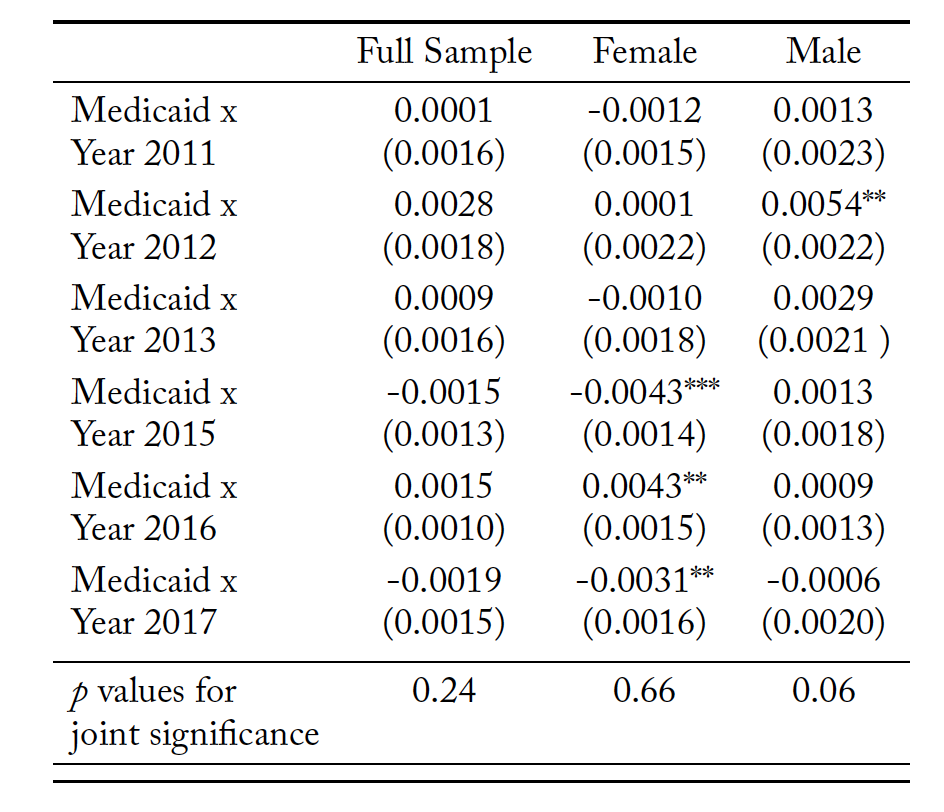
First, I test for the common trend assumption more formally with an event study. The results are provided in tables 4 and 5 for new marriages and new divorces, respectively. I jointly test the null hypothesis that all pre-2014 interaction terms are equal to zero using an F-test. I cannot reject the hypothesis that all pre-2014 interaction coefficients are jointly equal to zero for the full sample and the sample restricted to women for new marriages. However, I can reject the null for males since one of the pre-2014 coefficients is significant. These results instill confidence in a causal interpretation of the regression estimates for new marriages. As mentioned earlier, the event study rejects the null that all pre-2014 estimates are jointly equal to zero for the sample of new divorces. 5In addition to the event study analysis, I provide some additional supporting evidence for the identifying assumption, albeit not formally testable, through a placebo test. In this placebo test I estimate the main model specification using only the pre- treatment data and arbitrarily choose a point that cuts the pre-treatment window in half, thus creating an artificial Medicaid expansion date. I therefore choose years 2011–2014 in my sample, capturing marriages pre-Medicaid expansion between 2010– 2013. I also choose year 2013 and after as the artificial post period, as it cuts the pre-treatment window in half. I do not find an effect on new marriages engendering further evidence of common trends. (The coefficient is -0.0014 with a standard error of 0.0012 and is not significant at the 1, 5, or 10 percent levels of significance.)
Table 4. Newly Married Event Study Estimates
Source: American Community Survey.
Notes: The sample is restricted to non-elderly adults above 26 years of age with a high school diploma or less, who got divorced in the past 12 months, and all those who remained married, for each calendar year. Regression includes demographic, family, income, and unemployment controls. P values using wild bootstrap clustering method are reported. The symbol *** shows significance at the 1 percent level, ** is significant at the 2 percent level, and * is significant at the 10 percent level.
Table 5. Newly Divorced Event Study Estimates
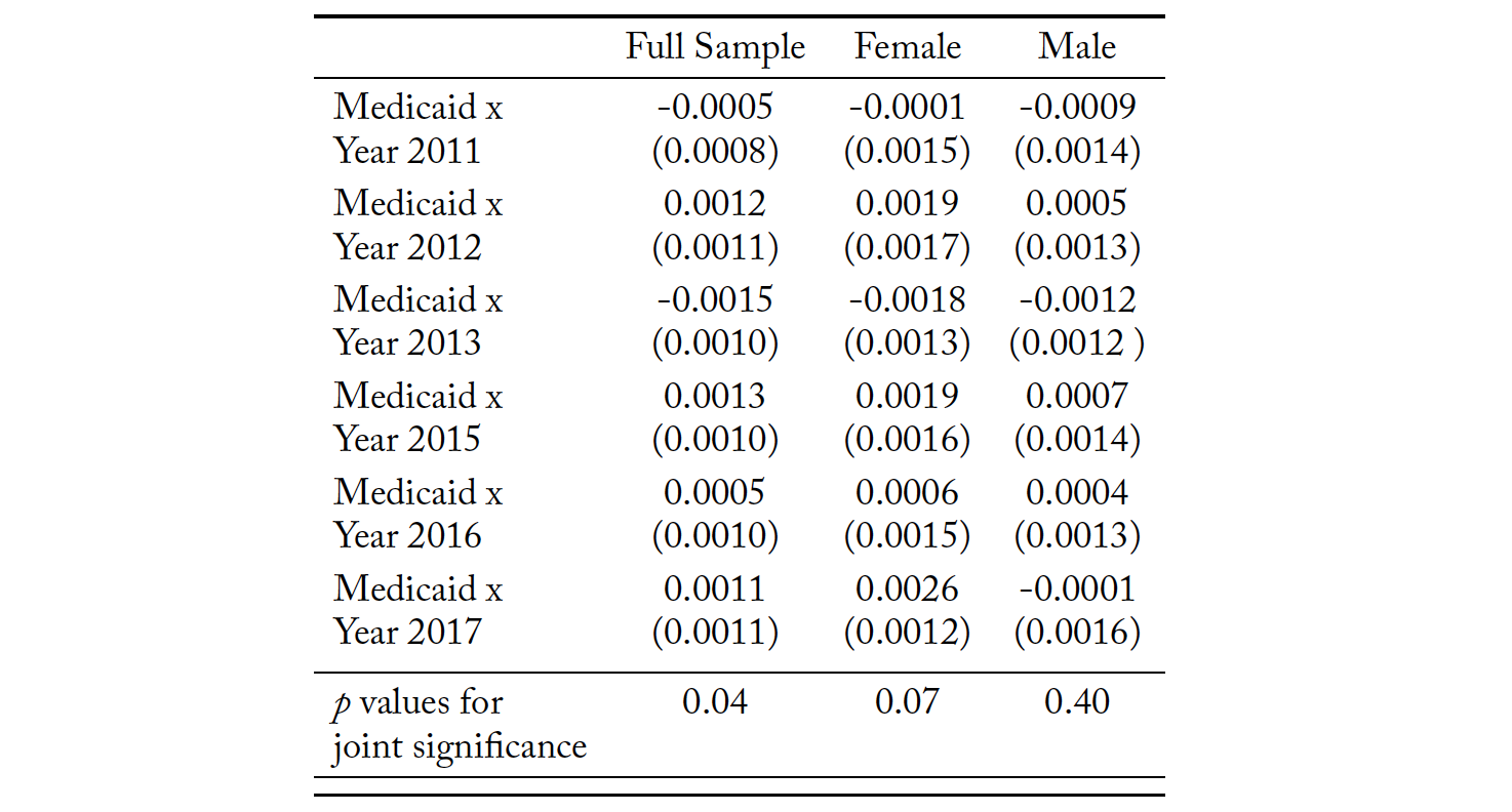
Source: American Community Survey.
Notes: The sample is restricted to non-elderly adults above 26 years of age with a high school diploma or less, who got married or stayed unmarried in the calendar year previous to the survey year. The base year for the event study is 2014 survey year (i.e., 2013 calendar year). The symbol *** indicates significance at the 1 percent level, ** is significant at the 2 percent level, and * is significant at the 10 percent level.
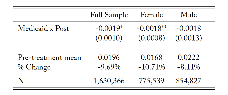
Second, in table 6, I define the eligibility of non-elderly adults above 26 years of age using low income (i.e., less than 138 percent of FPL) instead of low education as I used in the baseline model. The estimates are qualitatively similar compared to those from table 8, although they are statistically insignificant for the full sample. Women still show a decrease in new marriages by 8.2 percent, although it is smaller than the estimate in the low education sample.
Table 6. Newly Married Difference-in-Differences Estimates for Low-income Sample
Source: American Community Survey.
Notes: The sample is restricted to non-elderly adults above 26 years of age with income below 138 percent of FPL, who got married or stayed unmarried in the calendar year previous to the survey year. The symbol *** indicates significance at the 1 percent level, ** is significant at the 2 percent level, and * is significant at the 10 percent level.
Third, I estimate a logit model instead of the baseline linear probability model for the binary outcome variable. The odds-ratio of an interaction term is problematic for the interpretation of the size of the treatment effect due to non-linearity of the logit model (Karaca-Mandic, Norton, and Dowd 2012) since the log of a difference is not the same as the difference of the logs. However, Puhani (2012) shows that in a non-linear DD, the cross-difference captures the incremental effect of the coefficient of the interaction term. Moreover, in case of a logit model, the sign of the treatment effect is equal to the sign of the coefficient of the interaction term. I report the estimates in table 7.
Table 7. Logit Model Estimates for Newly Married
Source: American Community Survey.
Notes: The sample is restricted to non-elderly adults above 26 years of age with income below 138 percent of FPL, who got married or stayed unmarried in the calendar year previous to the survey year. The symbol *** indicates significance at the 1 percent level, ** is significant at the 2 percent level, and * is significant at the 10 percent level.
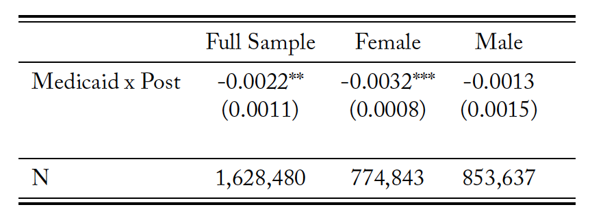
As a fourth sensitivity check, I use an alternate measure of new marriages. I use the variable that records whether a person got married in the 12 months prior to the time they were surveyed. As discussed before, this is a less accurate measure than the one used in my baseline model, but it can be reasonably expected to give qualitatively similar results. Table 8 shows the results are qualitatively the same, with women driving the decrease in new marriages.
Table 8. Difference-in-Differences Estimates with Alternate Definition of Newly Married
Source: American Community Survey.
Notes: The sample is restricted to non-elderly adults above 26 years of age with income below 138 percent of FPL, who got married in the last 12 months or stayed unmarried in the survey year. Regression includes demographic and unemployment controls. The symbol *** indicates significance at the 1 percent level, ** is significant at the 2 percent level, and * is significant at the 10 percent level.
Finally, I check the robustness of the results by dropping states having different degrees of early expansion prior to 2014 as per Courtemanche et al. (2017). I first drop five states (DE, DC, MA, NY, VT) that had relatively complete expansions prior to 2014 according to Kaestner et al. (2017). I then drop states that had partial expansion prior to 2014—14 in the treatment group and 4 in the control group. I then drop all early expanders to have only states that expanded in or after 2014. I employ a a wild cluster bootstrap resampling method here as well to account for the fact that there are smaller numbers of clusters, having dropped early expanders. The results are robust to this sample selection, implying that the effects are not differentially driven by states that expanded Medicaid (partially or more completely) prior to 2014. The estimates are provided in table 9.
Table 9. Newly Married Difference-in-Differences Estimates by Dropping Early Expansion States
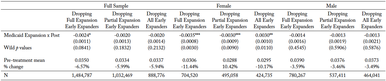
Source: American Community Survey. Notes: Wild p value is the corresponding p value using the wild bootstrap. The symbol *** indicates significance at the 1 percent level, ** is significant at the 2 percent level, and * is significant at the 10 percent level.
6 Conclusion
This study looks at the impact of the ACA Medicaid expansion on marital decision-making.. The results are suggestive of low-educated adults over 26 years of age substituting away from coverage as dependents through marriage in the presence of an alternative source of coverage through Medicaid. The estimated figure for the sample is a 6.92 percent reduction in marriage initiation. This adds to the broader discussion on whether economic incentives can have an impact on marital decision-making. Results indicate that economic incentives that change the costs and benefits associated with entering marriage can affect outcomes. Moreover, by extending the discussion to non-elderly adults other than young adults, this study is not restricted to studying marital behavior for a particular age group only.
Even though I do not find heterogeneous effects by sex, the fact that the effects are significant and larger in magnitude for the subsample of women (at an 11.6 percent drop in new marriages) is suggestive of the dependence that women have on their spouses for coverage. It also underscores their vulnerability to loss of coverage in the event of marriage dissolution, as has been discussed in earlier studies. While I cannot discern whether the increase in divorces can be completely attributed to Medicaid expansion, the decrease in new marriages can be interpreted as an indirect validation of the vulnerability of women to loss of coverage owing to marriage dissolution.
The Medicaid expansion may also affect same-sex marriages. These can be explored in conjunction with the state-specific timing of legalization of same-sex marriages to investigate if states that had legalized same-sex marriages at the time of Medicaid expansion differed in outcomes from states that did not. The results may also have implications on fertility, which has not been explored as of yet. If individuals choose to substitute away from marriage or defer marriage, it may have effects on fertility and childbearing.
Another area for further research could be the impact of other regulations of the ACA, such as insurance market reforms and sliding scale subsidies, to get a more holistic understanding of the impact of the ACA on marital decision-making and family structure. As Abramowitz (2016) points out, the multiple moving pieces of the ACA may counteract each other, making impact identification challenging. Thus, use of a novel methodology to disentangle the effects of the various limbs of the ACA may be an area of future research.
References
Abraham, J., and A. Royalty. 2005. “Does Having Two Earners in the Household Matter for Understanding How Well Employer-based Health Insurance Works?” Medical Care Research and Review 62 (2): 167–86.
Abramowitz, J. 2016. “Saying, ’I Don’t’: The Effect of the Affordable Care Act Young Adult Provision on Marriage.” Journal of Human Resources 51 (4): 0914-6643R2.
Angrist, J. D., and J. S. Pischke. 2008. Mostly Harmless Econometrics: An Empiricist’s Companion. Princeton, NJ: Princeton University Press.
Barkowski, S., and J. S. McLaughlin. 2020. “In Sickness and in Health: Interaction Effects of State and Federal Health Insurance Coverage Mandates on Marriage of Young Adults.” Journal of Human Resources 55 (2).
Becker, G.S 1973. “A Theory of Marriage: Part I.” Journal of Political Economy 81 (4): 813–46. Becker, G. S., 2009. “A Treatise on the Family.” Harvard university press.
Brooks, T., L. Roygardner, S. Artiga, O. Pham, and R. Dolan. “Medicaid and CHIP eligibility, enrollment, and cost sharing policies as of January 2019: Findings from a 50-state survey.” Kaiser Family Foundation.
Buchmueller, T. C., and R. G. Valletta. 1999. “The Effect of Health Insurance on Married Female Labor Supply.” Journal of Human Resources 34 (1): 42–70.
Cameron, A. C., J. B. Gelbach, and D. L. Miller. 2008. “Bootstrap-based Improvements for Inference with Clustered Errors.” Review of Economics and Statistics 90 (3): 414–27.
Chen, T. 2018. “Health Insurance Coverage and Marriage Behavior: Is There Evidence of Marriage-Lock?” Working paper. https://tianxuchen.weebly.com/uploads/2/2/8/1/22817854/marriage_lock_tianxu_chen_12282018.pdf.
Chen, T. 2019. “Health Insurance and Marriage Behavior: Will Marriage Lock Hold under Healthcare Reform?” Working paper. https://tianxuchen.weebly.com/uploads/2/2/8/1/22817854/chen_ma_reform_04152019.pdf.
Courtemanche, C., J. Marton, B. Ukert, A. Yelowitz, and D. Zapata. 2017. “Early Impacts of the Affordable Care Act on Health Insurance Coverage in Medicaid Expansion and Non‐expansion States.” Journal of Policy Analysis and Management 36 (1): 178–210.
Gibson-Davis, C. M., K. Edin, and S. McLanahan. 2005. “High Hopes but Even Higher Expectations: The Retreat from Marriage among Low-income Couples.” Journal of Marriage and Family 67:1301–12.
Gruber, J. 2011. “The Impacts of the Affordable Care Act: How Reasonable Are the Projections?” NBER Working Paper No. 17168, National Bureau of Economic Research, Cambridge, MA.
Hampton, M., and O. Lenhart. 2019. “The Effect of the ACA Medicaid Expansion on Marriage Behavior.” Working paper. https://ssrn.com/abstract=3450609.
Heim, B., I. Lurie, and K. Simon. 2018. “The Impact of the Affordable Care Act Young Adult Provision on Childbearing: Evidence from Tax Data.” Demography 55 (4): 1233–43.
Hu, W. Y. 2003. “Marriage and Economic Incentives: Evidence from a Welfare Experiment.” Journal of Human Resources 38 (4): 942–63.
Kaestner, R., B. Garrett, J. Chen, A. Gangopadhyaya, and C. Fleming. 2017. “Effects of ACA Medicaid Expansions on Health Insurance Coverage and Labor Supply.” Journal of Policy Analysis and Management 36 (3): 608–42.
Karaca-Mandic, P., E. C. Norton, and B. Dowd. 2012. “Interaction Terms in Nonlinear Models.” Health Services Research 47 (1): 255–74.
Lavelle, B., and P. J. Smock. 2012. “Divorce and Women’s Risk of Health Insurance Loss.” Journal of Health and Social Behavior 53:413–31.
Peters, E., K. Simon, and J. Taber. 2014. “Marital Disruption and Health Insurance.” Demography 51:1397–1421.
Puhani, P. A. 2012. “The Treatment Effect, the Cross Difference, and the Interaction Term in Nonlinear ’Difference-in-Differences’ Models.” Economics Letters 115 (1): 85–87.
Simon, K., A. Soni, and J. Cawley. 2017. “The Impact of Health Insurance on Preventive Care and Health Behaviors: Evidence from the First Two Years of the ACA Medicaid Expansions.” Journal of Policy Analysis and Management 36:390–417.
Slusky, D., and D. Ginther. 2017. “Did Medicaid Expansion Reduce Medical Divorce?” NBER Working Paper No. 23139, National Bureau of Economic Research, Cambridge, MA.
Sohn, H. 2015. “Health Insurance and Risk of Divorce: Does Having Your Own Insurance Matter?” Journal of Marriage and Family 77:982–95.
Wellington, A. J., and D. A. Cobb-Clark. 2000. “The Labor Supply Effect of Universal Health Coverage: What Can I Learn from Individuals with Spousal Coverage?” Research in Labor Economics 19:315–44.
Yelowitz, A. 1998. “Will Extending Medicaid to Two-parent Families Encourage Marriage?” Journal of Human Resources 33:833–65.
Zimmer, D. 2007. “Asymmetric Effects of Marital Separation on Health Insurance among Men and Women.”Contemporary Economic Policy 25:92–106.