Warding Off Development: Local Control, Housing Supply, and NIMBYs

Mast, Evan

Introduction

Housing construction in the United States has not kept pace with demand. Freddie Mac (2018) estimates that 2017 production fell 20% short of the level required to accommodate population growth and replace dilapidated structures. This not only affects housing markets, where costs continue to rise faster than incomes (Albouy et al. 2016), but may also slow aggregate economic growth (Hsieh and Moretti 2019). Accordingly, ways to address this shortfall have come to the forefront of the policy debate.

The highly decentralized control of land-use regulation and development approval may create a classic NIMBY (not-in-my-backyard) problem that contributes to the shortfall. Because new housing has diffuse benefits and concentrated costs—such as congestion, lost green space, and construction noise—people may prefer less construction near their residence than would be optimal for the town or region. Moreover, citizens can use their outsized influence over proposals in their area to restrict production. Towns within a region can use locally controlled land-use regulations to behave similarly. Anecdotally, these forces seem to be strong, leading to recent reforms that reduce local control of land-use regulations in an attempt to increase housing supply.¹ However, there is little empirical evidence on how local control of regulation affects housing supply, likely because of the difficulty of isolating relevant exogenous variation.

In this paper, I obtain causal estimates of the effect of increased local control on housing production by exploiting a common reform to town council elections. The reform is a change from “at-large’’ elections, in which citizens vote for candidates to represent the town as a whole, to “ward” elections, in which the town is divided into wards and each citizen votes for a single candidate to represent their area. This change decentralizes town governance, as at-large representatives should be responsive to the town’s median voter, while ward representatives should respond to the median in their district. Moreover, informal practices like logrolling and aldermanic privilege often give ward representatives significant control over issues in their district, due to deference from their counterparts in other wards (Schleicher 2013).

I use a difference-in-differences (DiD) approach to evaluate the effect of switching from at-large to ward voting.² The baseline specification uses all initially at-large towns as a control group and includes county-year fixed effects to account for granular spatial trends.³ However, causal identification is complicated by the fact that towns choose their election type, making switches endogenous. Historically, this choice has been strongly influenced by racial dynamics. White majorities used at-large systems to limit minority representation, creating equity concerns that led to court cases and legislation in the 1980s that caused many towns to switch to ward voting (Trebbi et al. 2008). Towns that switched are thus on average bigger and less white than towns that remained on at-large voting. However, their housing markets are similar, consistent with evidence that housing concerns rarely motivate switches (Hankinson and Magazinnik 2019), and demographic pre-trends are similar within counties, supporting the parallel trends identification assumption.

Event study results show that, prior to changing to ward voting, treated and control towns were on very similar housing production trends. However, the number of units permitted falls sharply in treated towns immediately upon the reform’s approval, leading to a DiD estimate of -24%. Significant heterogeneity underlies this average effect—effects are larger (-47%) for multi-family units and in towns with higher owner-occupancy rates. This is consistent with anecdotally stronger development opposition from homeowners (Fischel 2001) and toward larger projects. Results are similar using a matched control group or including only treated towns in the sample, alleviating concerns about pre-existing differences between treatment and control towns. While I cannot determine the relative importance of ward representatives blocking projects in their district and ward councils passing more restrictive regulation, extensions suggest that results are not driven by indirect effects of non-housing policy.

I also consider units financed using federal Low-Income Housing Tax Credits (LIHTC). While the average effect on permitting any LIHTC units is zero, point estimates are negative in high-homeownership towns and positive in others. Diamond and McQuade (2019)’s finding of positive effects of LIHTC on home values in low-income areas and negative in high-income areas suggests an explanation. Ward voting in wealthy high-ownership areas could empower residents who want to protect their property values, while, in low-ownership places, it allows low-income districts to gain representation and advocate for the benefits of LIHTC.

On the whole, more localized control severely reduces housing production, which has important policy implications for areas trying to increase supply. Towns with ward elections may need to increase the set of structures can be built “as-of-right” (without a special approval process) or reduce the formal and informal policies giving council members more power over developments in their district. Extrapolating to a parallel setting, regional organizations or state governments may need to set minimum standards for housing production or limits on the restrictiveness of municipal land-use regulations.

The most directly related literature studies land-use regulation and housing markets. As reviewed in Gyourko and Molloy (2015), many studies have shown a robust relationship between tighter regulation and lower housing construction, as well as higher prices.⁴ I first add to this literature by providing a
quasi-experimental analysis of the switch from at-large to ward elections, which, given the power of town councils in this setting, is reasonable to consider as a change to land-use policy. In addition, like Parkhomenko (2018) and Duranton and Puga (2019), this paper connects endogenous local land-use regulations and housing approval to the underlying institutions and economic forces that generate them, empirically showing the importance of local control and NIMBYism. Concurrent work by Hankinson and Magazinnik (2019) is most closely related. They use more spatially detailed data to identify a large negative effect of ward voting on multi-family units in California between 2010 and 2018, as well as a shift in permit location within towns, while I use a longer national sample that provides more precise, representative, and long-run estimates.⁵

More broadly, this paper contributes to the literature on decentralization and fiscal federalism. Most directly related is the NIMBY literature, which has largely focused on mechanisms to fairly allocate socially necessary but locally undesirable land-uses (Frey et al. 1996, Feinerman et al. 2004, Levinson 1999). This study is among the first to obtain a causal estimate of how changes to local control affect the quantity of such a land-use.

1 Background on Electoral Reforms

1.1 At-Large and Ward Elections

Towns in the U.S. generally use one of two methods to aggregate individual votes into seats on their council. In at-large elections, each citizen chooses from the same pool of candidates to elect representatives who represent the town as a whole. In ward elections, the city is divided into smaller wards (or districts) in which each citizen votes for a single candidate to represent their area. About two-thirds of towns use at-large elections for town council, about 15% of towns use a purely ward system, and 20% have some representatives elected at-large and some by ward (Clark and Krebs 2012).

Towns are able to choose between different election types, and a literature in both political science and economics studies the determinants of that choice. In theory, any majority bloc—whether defined by race, ideology, or ethnicity—can suppress the representation of a minority bloc through at-large voting (Davidson and Korbel 1981). For example, a minority representing 15% of the population may not be able to win a seat in an at-large election, but could constitute a majority within a smaller ward. In recent years in the United States, the majority and minority have typically been defined by racial lines. Trebbi et al. (2008) show that majority-white Southern towns implemented at-large systems after African American voting rights were strengthened by the Voting Rights Act, and a number of studies have found that ward voting indeed increases the representation of racial minorities.⁶

Accordingly, changes between the two electoral rules have often been motivated by racial equity concerns. A key 1982 Supreme Court case held that at-large elections in Burke County, Georgia, violated the Fourteenth Amendment rights of African-Americans in the county, sparking a wave of switches to ward voting in the 1980s and 1990s.⁷ While there are other reasons towns may switch to ward voting, in the 1991 Form of Government Survey from the International City/County Management Association, 31% of the 77 switching towns cite either a court or state mandate. An additional 20% cite a government initiative, 29% a referendum, and 21% another (unlisted) reason. Of course, these other reforms could also have been indirectly motivated by court precedent. Importantly, housing markets are, to my knowledge, rarely cited as an inspiration for reform, as Hankinson and Magazinnik (2019) carefully document in the meeting minutes of several California cities that switched to ward voting.

1.2 Diﬀerences in Representative Incentives

Ward systems are more decentralized than at-large, since representation is tied to smaller groups of people. This leads ward and at-large representatives to face very different incentives. In classic models, at-large representatives are responsive to the town’s median voter, while ward representatives should respond to the median voter in their district.⁸ This difference is likely important for housing approvals. Within the ward containing a proposed development, a higher percentage of people will be affected by the project’s concentrated costs—such as construction noise, lost green space or views, and congestion—than in the town as a whole. This means that the ward’s median voter will have a more negative opinion of a proposal than the town’s median voter, making ward representatives less likely to support housing developments.

However, differences between the two systems go beyond changes to the median voter. In ward systems, the representative for the district containing a proposed development often has a disproportionate influence over its approval due to logrolling and “aldermanic privilege,” informal practices in which council members defer to the home representative and, in return, receive the same treatment when an issue arises in their ward. This dynamic not only increases the power of ward representatives, but may also lead ward councils to pass more restrictive land-use regulation in general, in order to increase the proportion of projects requiring special council approvals and further expand their influence over their district.

Because housing is such a local issue, decentralization even within one town can have important effects. Of course, similar forces apply at other geographic levels. For example, allowing towns instead of counties or other regional bodies to set land-use regulations could decrease housing supply, since a town also absorbs more of a new development’s costs and fewer of its benefits than a larger region. More broadly, decentralization leads to similarly misaligned local and regional incentives in many classic NIMBY problems.

2 Data and Sample Construction

2.1 Data Sources

a. ICMA Data: Electoral reforms are identified using the International City/County Management Association (ICMA) Municipal Form of Government survey. The ICMA surveys towns (identified by Census Place codes) on their election type and form of government every five years and receives approximately 3,500–5,000 responses.⁹ Trebbi et al. (2008) also use this data to study changes in electoral rules and show that the sample is representative of the set of U.S. towns with population over 2,500.¹⁰

To identify changes from at-large to ward voting, I use the survey question that asks whether a town made this change in the past five years, and, if so, when the reform was approved.¹¹ Across seven waves of the survey (from 1981 to 2011), this identifies nearly 300 municipalities that switched from at-large to purely ward elections at some point between 1970 and 2011. These switches occur across all decades, with 112 and 103 in the 1980s and 1990s and 21 and 30 in the 1970s and 2000s. Appendix Figure A.1 shows the full distribution across years.

Because the survey has an imperfect response rate, this approach will miss some changes in electoral rules. However, given the relative infrequency of reforms among survey respondents (<1%), this should be a small proportion of the control group. In addition, the control group ultimately includes only towns that always report at-large voting, further minimizing the issue. Finally, while some towns do report switching from ward to at-large systems, it is much less common, so much so that ICMA does not ask about these switches in most waves of the survey. In robustness checks, I probe the treatment definition and, to the extent possible, also consider ward to at-large switches.

b. Census Building Permit Data: Census Place-level data on new housing permits comes from the 1980 to 2018 waves of the Census Bureau Building Permit Survey. Each year, the Census Bureau surveys about 20,000 permit-granting local governments that represent 98% of U.S. housing production. The Census’s follow-up surveys show that almost all permitted units are eventually built, making the permits a reasonable measure of housing construction. The data includes both the total number of units permitted and the number permitted in single-family and multi-family structures.¹² Appendix Figure A.2 shows the time series of units permitted, which is highly correlated with the business cycle, as expected.

c. LIHTC Data: Data on buildings receiving Low-Income Housing Tax Credit (LIHTC) financing is provided by the Department of Housing and Urban Development and covers all LIHTC buildings permitted between 1986 and 2015, providing details such as number of units in each building and percent of units at various levels of income restriction. I aggregate these to the Census Place level in order to merge with the other data sets.

2.2 Sample Construction

I merge these three data sources to construct the analysis sample. After removing unincorporated areas from the building permit data, roughly 16,000 towns can be linked across all years of the survey. Of these, I keep only the 5,830 that can be matched to at least one ICMA survey wave. Next, about 6.5% of town-years and 60% of towns are matched to at least one LIHTC project, and I assume that town-years in the time frame covered by the LIHTC data that are not matched to the LIHTC data saw no such units permitted.

I then apply several restrictions to complete the final analysis sample. First, I drop town-years with population below 2,500, which are poorly represented in the ICMA data. Second, in order to improve the comparability of the treatment and control groups, I keep only towns that either report switching from at-large to ward or always report at-large voting. Third, for simplicity, I drop the additional 46 towns that switch from at-large to a mixed system with some ward and some at-large representatives.¹³ The final sample contains approximately 2,500 towns in the years 1980–2018 and includes 240 at-large to ward transitions.

3 Empirical Strategy

3.1 Baseline Speciﬁcation

I study the effect of changing to ward voting using a difference-in-differences strategy. The outcome variables are measures $y$ of regular and low-income housing permits, and the treated group is towns that made this switch. In the baseline specification, the control group is all at-large voting towns, and I include county-year fixed effects to non-parametrically control for local trends. In alternative specifications, I show that using a matched control group or including only treated towns return similar results.

In order to investigate pre-trends and effect dynamics, I first estimate the following event study specification for town $i$ in county $c$ in year $t$ :

(1) $\begin{equation*} y_{it}=\gamma_i + \alpha_{ct} + \sum_{k \in C} \beta_k d_{it}^k + \epsilon_{it}. \end{equation*}$

I define $C$ and $d_{it}^k$ such that the d variables represent time-to-treatment dummies with a two-year window. This requires $C$ = { -8, -6, -4, -2, 0, 2, 4, 6, 7 } and

$d_{it}^k = \begin{cases} \math{1}[t \leq t^*_i - 8 ] & if \; k = -8 \\ \math{1}[t^*_i + k -1 \leq t \leq t^*_i + k ] & if \; -8<k<7 \\ \math{1}[t \geq t^*_i + 7 ] & if \; k = 7 \\ \end{cases}$

for a town that approved the reform in year $t^*$ and 0 for other towns. Because reforms are likely under discussion for some time prior to approval, potentially affecting permits prior to $t^*$ , I set 2–3 years before the reform as the omitted coefficient. I also include only years from 1980 to 2003 (recall that the treatment variable is observed from 1970 to 2011) to ensure that all $d_{it}^k$ are correctly defined, following Schmidheiny and Siegloch (2019).

Following the event study, I estimate an average effect of treatment by replacing the years-to-treatment dummies with a single after-treatment dummy:

(2) $\begin{equation*} y_{it}=\gamma_i + \alpha_{ct} + \beta \math{1}(t \geq t^*_i) + \epsilon_{it}. \end{equation*}$

Recent work has pointed to problems with difference-in-differences with staggered treatments.¹⁴ A theme across these papers is that the estimator may not yield a sensible weighted average if treatment effects are heterogeneous over time or if the specification implicitly uses already-treated units as a large share of its control units. To minimize these problems, I drop town-years that are more than seven years after treatment from this specification, and I discuss related robustness checks with the main results.

Because of the skewed distribution of units permitted, I use the log of units (plus one) as the dependent variable for market-rate units. Fewer than 10% of town-years have no permits, mitigating potential issues with the discontinuity at zero. For LIHTC units, I instead use an indicator for whether a town permitted any LIHTC units in a year. This is because the number of LIHTC units permitted in a town-year is very lumpy—fewer than 10% of town-years permit any units, but those that do permit an average of 101. Finally, in all specifications, standard errors are clustered at the state level.

3.2 Identiﬁcation

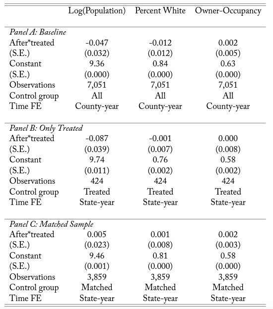
In the baseline specification, the identification assumption is that, in the absence of an electoral reform, housing permits would have changed in parallel for towns that switched from at-large to ward voting and other initially at-large towns in the same county. The primary threats to this assumption arise because towns generally choose if and when to make this switch (or are compelled by the courts). I investigate this assumption in Table 1.

In Panel A, I regress several characteristics on an indicator for whether a town ever switches, and, depending on the specification, either county-year or year fixed effects.¹⁵ Because characteristics are only observed in the decennial census years, I include only those years in the sample, and I drop post-reform observations in treated towns to avoid conflating baseline differences and the treatment effect. Towns that switch are significantly larger and less white on average, which makes sense given that reforms are often motivated by concerns about under-representation of non-white populations, implying that switching towns must have some presence of these groups. However, the difference in housing units permitted per capita is near zero when including county-year effects, and the difference in the rate of homeownership is only 6% on a base of 62%. This similarity in housing markets fits with anecdotal evidence that reforms are typically not driven by housing concerns.

Although levels of characteristics suggest the decision to switch to ward voting is not random, this does not necessarily violate the parallel trends identification assumption. Panel B of Table 1 assesses differences in trends by repeating the exercise in Panel A using ten-year changes in town characteristics as the dependent variable. With the county-year fixed effects used in the baseline specification, the treatment indicator is statistically insignificant for all outcomes, suggesting that treated towns were evolving similarly to towns in the same county—the relevant comparison for the identification assumption. In addition to the exercises in this table, the event study plots presented with the main results show parallel trends in housing production during the pre-period, further supporting the identification assumption.

3.3 Alternative Speciﬁcations

Although treated and control towns within counties appear to be on similar trends, the differences in size and racial composition motivate two alternative specifications. First, I include only towns that undergo a reform at some point during the sample. Because this shrinks the sample greatly, I coarsen the time fixed effects to state-year. The concern in this specification is that the timing of the decision to switch to ward voting may be correlated with changes in housing development. To assess this, I restrict to the sample of treated towns and regress changes in town characteristics on a dummy for the decade prior to a reform and a set of town fixed effects, as well as either year or state-year fixed effects. The coefficients of interest, shown in Panel C of Table 1, are all small and statistically insignificant, suggesting that reform timing is not correlated with changes in local housing markets.

In the second alternative specification, I construct a control group of at-large towns that are observably similar to the switching towns. I match each switching town to its five nearest neighbors among at-large towns in the same state, based on population, percent white, and percent homeownership, all measured in 1980.¹⁶ I do this with replacement, allowing control towns to be matched to multiple treatment towns. I then include all towns that are matched to any treatment town in the control group. Because this sample is smaller than the baseline, I again coarsen the time fixed effects to state-year.

4 Results

4.1 Main Results

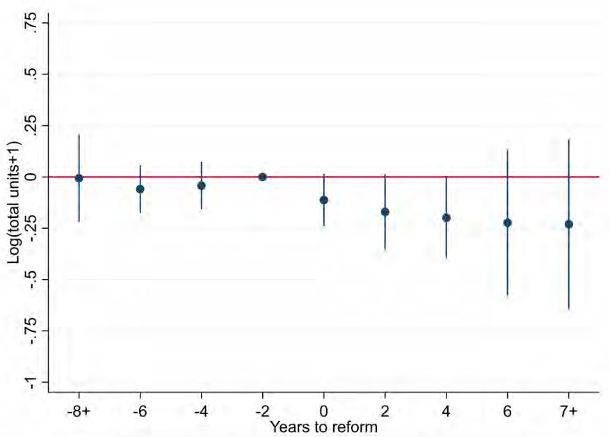
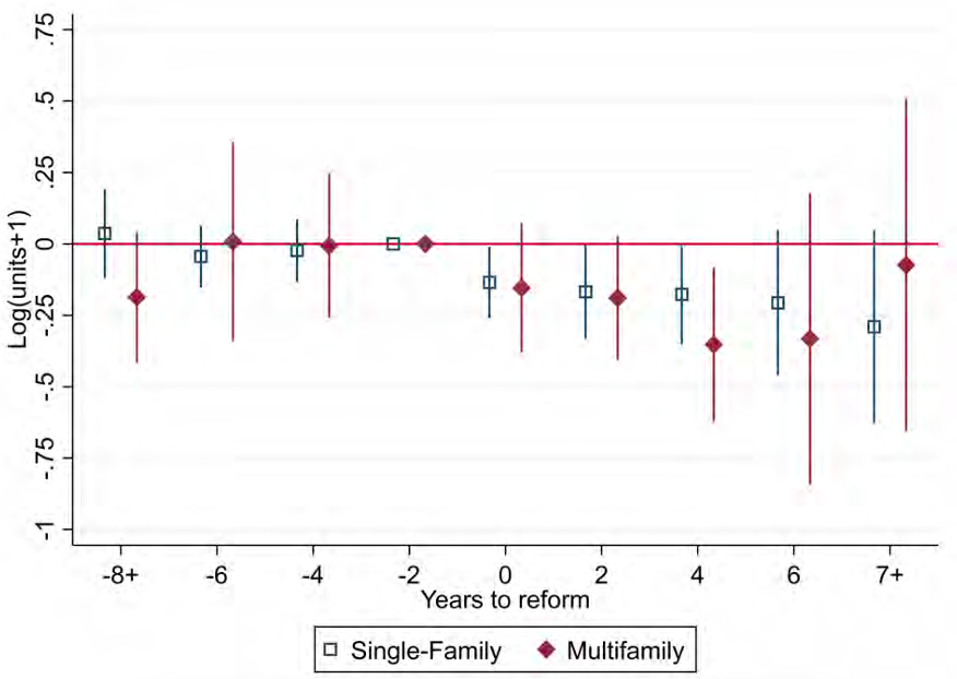
Baseline event study results for log housing units permitted plus one are shown in Figure 1. Pre-trends appear to be minimal, suggesting that at-large towns serve as an effective control group despite being different on some characteristics. However, there is a stark change following the reform’s approval, with housing permits falling in treated towns. The effect appears to begin immediately in the treatment year and reach a stable level by two years later, where it remains until the end of the sample. Figure 2 repeats the event study specification separately for single-family and multi-family units. While the pattern of parallel pre-trends followed by a sharp decline is the same for both outcomes, the effect is much larger for multi-family units. In addition, for multi-family units, the effect is less stable in the post-period, perhaps because the lumpy nature of multi-family buildings creates more noise.

The difference-in-differences results shown in Panel A of Table 2 approximate the average effect of decentralization over the seven years after the reform. The after-treatment coefficient is -0.236 (S.E. = 0.059, p<0.01) when using all units as the outcome variable, suggesting that reforms reduced housing permits by over 20%.¹⁷

The median number of units permitted in a year is 25, pointing to an absolute decrease of about 5 units. The estimates for single- and multi-family units are -0.118 (S.E. = 0.055, p=.04) and -0.478 (S.E. = 0.145, p<0.01), consistent with the larger change observed in the multi-family event study. The larger estimates for multi-family could occur either because neighbors oppose larger projects more strongly, or because the approval process for multi-family is often more onerous and could provide more opportunities for a ward representative to block a project.

Next, I turn to LIHTC permits. Column 4 of Panel A of Table 2 shows the baseline effect on the probability that any LIHTC units are permitted, which is less than a tenth of a percent. The underlying event study plot, shown in Appendix Figure A.3, does not suggest that this null average effect masks any interesting time trends. However, as discussed below in Section 4.3, there is important heterogeneity across towns underlying the overall effect.

Results from alternative specifications support the baseline estimates. The DiD estimates are extremely similar when including only treated towns (Table 2, Panel B), and the corresponding event studies (Appendix Figures A.4 and A.5) also change minimally. When using a matched control group, estimates are smaller but tell a similar story (Panel C of Table 2, Appendix Figures A.6 and A.7). Total units decline by 12.3% (S.E. = 0.041, p=.06) and multi-family units decline by 22.9% (S.E. = 0.065, p<0.01). The effect on single-family units is negative but not statistically significant.¹⁸

A recent literature highlights a number of potential issues with DiD designs exploiting staggered treatments. Focusing first on the event study approach, Abraham and Sun (2019) show that the primary assumption required for consistent estimates is that treatment effect dynamics are similar across cohorts treated in different years. To investigate, I plot event studies including only towns treated before 1995 (representing the earlier 75% of towns) and only towns treated after 1986 (the later 75%) on the same axis in Appendix Figure A.8. The plots are encouragingly similar in both magnitude and dynamics.

Turning to the DiD specifications, estimates may be inconsistent if treatment effects change over time (Goodman-Bacon 2018, Callaway and Sant’Anna 2019). The stability of post-period coefficients in the event study plots is encouraging on this front. Heterogeneity across towns can also cause problems, as shown in de Chaisemartin and d’Haultfoeuille (2019), because the overall DiD estimate is a weighted average of subgroup effects that may include negative weights, which can lead the overall estimate to have a different sign than the underlying comparisons. However, following their suggested methodology to estimate the significance of negative weights in my baseline estimate, I find that only 2.1% of comparisons receive negative weight, summing to a total of -0.0000322. This suggests that the overall estimate represents a relevant combination of underlying effects.

4.2 Heterogeneity by Homeownership

Differences across towns in how decentralization affects housing markets may be important for how metropolitan areas grow, as well as the impact of reforms to land-use or local control. A wealth of research, as well as anecdotal evidence, suggests that NIMBYism is strongest in areas with high owner-occupancy rates. Homeowners may be particularly opposed to development because of their direct stake in property values, which could be reduced by increased supply or congestion effects, and because they are likely to remain in the area for longer than renters (Fischel 2001). Homeowners are also more likely to attend community meetings on new developments (Einstein et al. 2019) and less likely to support developments when the site is closer to their residence (Hankinson 2018).

To test the importance of homeownership, I repeat the baseline difference-in-differences specification, but allow switching towns with above-median ownership rates to have a different treatment effect. Adding this interaction term and a vector of year × above-median ownership fixed effects yields

(3) $\begin{equation*} y_{it}=\gamma_i + \alpha_{ct} + \kappa_{ht} + \beta_1 \math{1}(t \geq t^*_i) + \beta_2 \math{1}(t \geq t^*_i) \times \math{1}(h=1) + \epsilon_{it}, \end{equation*}$

where $h$ is an indicator for above-median owner-occupancy.

Results are shown in Table 3. For total market-rate permits, the interaction term is negative but statistically insignificant in all of the baseline, only-treated, and matched-control specifications. However, the estimates are much larger for multi-family units. The interaction term is -0.522 (S.E.=0.32, p=0.11) in the baseline, versus a -0.202 average effect, and -0.72 (S.E.=0.24, p<0.01) and -0.313 (S.E.=0.24, p=0.19) in the only-treated and matched sample specifications. Though these results are noisy and not all statistically significant, they provide suggestive evidence that the effect of ward voting on multi-family housing is larger in high homeownership towns.

Finally, Column 4 of Table 3 shows results for LIHTC permits. Interestingly, the null average effect found in the previous section appears to be composed of very different effects in low- and high-ownership places. In the baseline specification, the average effect is a statistically insignificant 0.029, and the interaction term is -0.074 (S.E. = 0.034, p<0.035). These sum to a total effect of -0.045 (S.E. = 0.018, p=0.02) for high-ownership towns. Similarly, in the matched specification, the average effect is positive but only marginally significant, while the interaction term is -0.052 (S.E. = 0.025, p=0.048). In contrast, both coefficients are near zero in the only-treated specification.

Although the results are not uniform across specifications, taking the point estimates seriously points to an interesting story: low-homeownership places increase LIHTC permits following electoral reforms, while high-homeownership towns instead decrease them. This pattern makes sense in light of research showing that the effect of LIHTC on nearby home prices is positive in low-income areas and negative in high-income areas (Baum-Snow and Marion 2009, Diamond and McQuade 2019), as well as Hankinson (2018)’s finding that homeowners are more likely to oppose low-income developments when close to their residence, while renters are not. Ward voting in low-ownership places could allow low-income districts to gain a seat on town council and advocate for the benefits of LIHTC in their area, while, in wealthy high-ownership towns, it primarily empowers nearby residents who want to protect their property values.

4.3 Mechanisms

Even given correct causal estimates, the underlying mechanism linking electoral reforms to housing supply may not be related to decentralization and NIMBYism. One possibility is that the administrative burden of changing electoral rules could slow the permitting process or cause developers to delay plans. However, it seems unlikely that this would persist for many years after the reform, and, as shown in Panel C of Appendix Table A.3, towns that switch from ward to at-large voting do not see decreased permits.

Alternatively, over a longer time period, a ward-elected council could set non-housing policies that make a town less attractive to developers. But the timing again does not support this story—the effect of the reform occurs immediately, before these policy changes could be implemented and pass through to construction. In addition, Appendix Table A.4 repeats the main difference-in-differences specifications using other town characteristics as the dependent variable. Across the three specifications and three dependent variables, only one estimate is statistically significant. This is inconsistent with large indirect effects of the reform that pass through to housing markets. Similarly, Column 3 of Appendix Table A.2 shows estimates of the effect on total units with added controls for time-varying town characteristics (percent white, percent owner occupancy, and population). The coefficients of interest are similar to the baseline specification, suggesting that indirect effects of reforms cannot explain the housing production result.

The strongest support for decentralization and NIMBYism as the causal mechanism may be the heterogeneity across towns and unit types. My proposed mechanism naturally explains the observed larger effects for multi-family units and in high-homeownership towns, while the most obvious alternatives do not. Finally, given the extent of town councils’ control over land-use regulation and their limited role in areas of policy handled by state and federal governments, it makes sense that their effect on the housing market would occur primarily through this channel.

5 Conclusion

The shortfall in housing construction has attracted increased attention as U.S. housing costs rise. A contributing factor may be that land-use regulation and development approvals are controlled at a very local level, and policymakers aiming to spur construction have begun to target this feature of housing policy. For example, Oregon has limited how restrictive municipal zoning regulation can be, and California has increased enforcement of state targets for local housing production. At the local level, Minneapolis eliminated single-family zoning, making it more difficult for ward representatives to block denser developments.

Despite the increased attention, there is little empirical evidence on the importance of local control of housing regulations. In this paper, I exploit changes in electoral rules that provide a rare source of exogenous variation in local control. My findings support conventional wisdom and anecdotal evidence of NIMBYism, as the reform reduces local housing production by over 20%. However, I emphasize two caveats. First, I do not measure potential welfare gains from more decentralized control, whether through housing markets or elsewhere (such as increased minority representation from ward voting). Second, while the forces underlying my proposed mechanism are quite general, I study a specific policy, and results may not generalize to every situation. Most proposed reforms consider decreasing local control, and applying my findings to this setting requires a symmetry assumption. Similarly, towns within a region are a parallel setting, but more research is needed to determine the effect of decentralization at that level of government.

Appendices

Figure 1. Baseline Event Study for Total Units Permitted

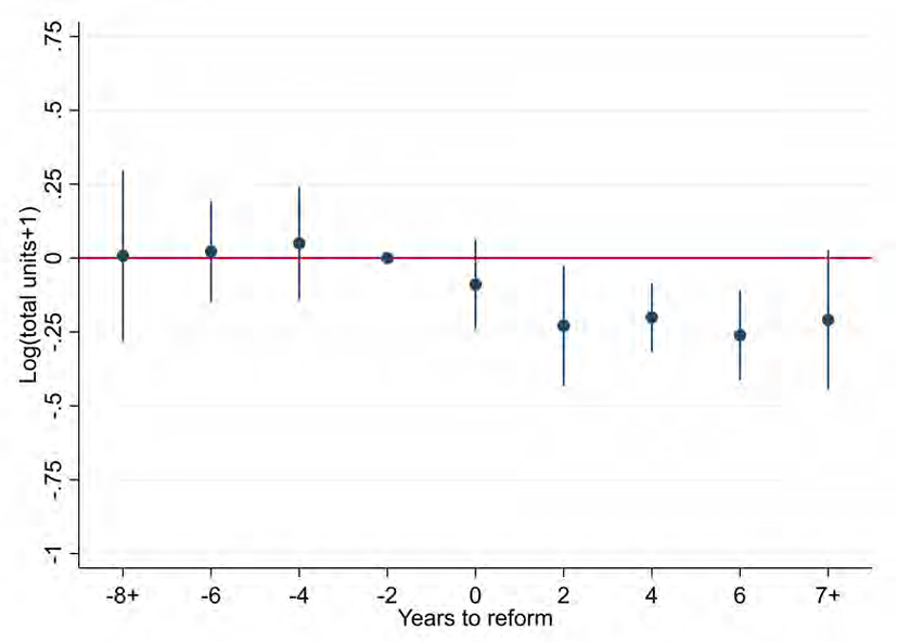
Note: This figure shows event study coefficients from the estimation of Equation 1 with log(total units + 1) as the dependent variable. Year 0 is the year that a town approved to a switch from at-large to ward elections. The dummies for years to treatment are bundled into two-year bins, and the label on the x-axis represents the later year. The specification includes town fixed effects, and errors are clustered at the state level.

Figure 2. Baseline Event Study for Single- and Multi-Family Units Permitted

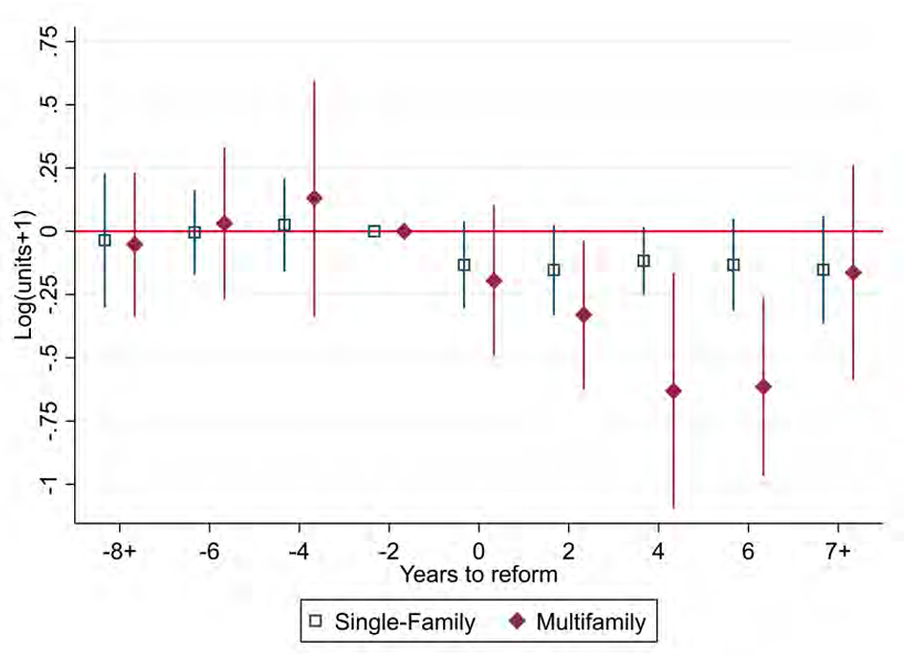
Note: The figure shows event study coefficients from two separate estimations of Equation 1, with log(single-family units + 1) and log(multi-family units + 1) as the dependent variables. Year 0 is the year that a town approved a switch from at-large to ward elections. The dummies for years to treatment are bundled into two-year bins, and the label on the x-axis represents the later year. The specification includes town fixed effects and county-year fixed effects, and errors are clustered at the state level.

Table 1. Comparison of Treatment and Control Towns

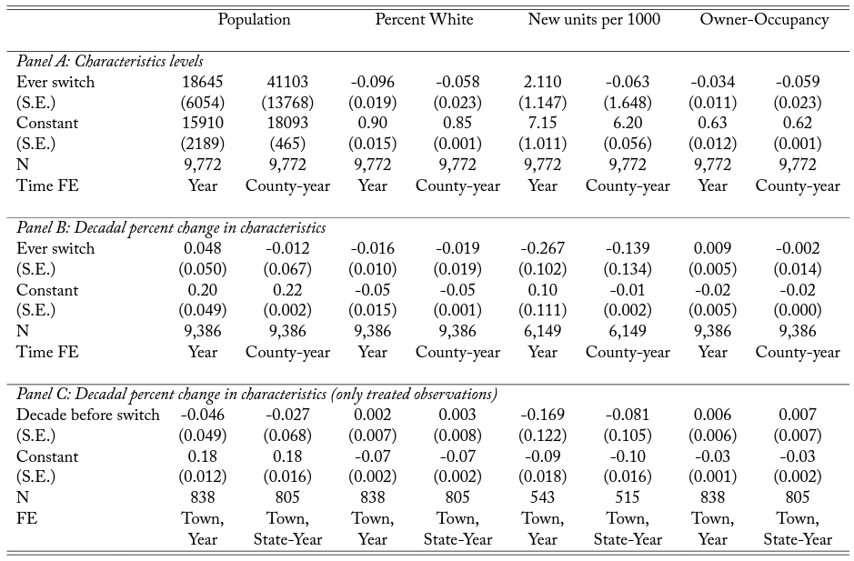
Note: This table compares characteristics of treatment and control towns. Panel A depicts regressions of the variable in the column heading on an indicator for if a town ever switches from at-large to ward voting, as well as a vector of either year or county-year fixed effects. Years after the reform are dropped for treated towns. Panel B repeats the exercise using decadal changes as the dependent variable. Panel C restricts to treated towns and regresses changes in the dependent variable on an indicator for the decade before the reform, as well as town and either year or state-year fixed effects. In all specifications, only decennial census years are included and errors are clustered at the state level.

Table 2. Difference-in-Differences Results

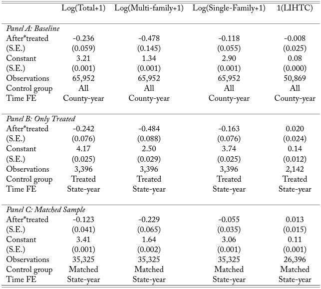
Note: This table shows results from the difference-in-differences specification in Equation 2. The column heading denotes the dependent variable. Panel A represents the baseline specifications, which includes the full analysis sample. Panel B includes only observations that are treated at some point in the sample period, while Panel C restricts to the matched sample described in Section 3.3. The specifications include town fixed effects and the time fixed effects indicated in each panel. Errors are clustered at the state level.

Table 3. Heterogeneity by Homeownership Rate

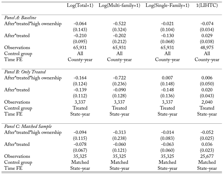
Note: This table shows how the effect of ward voting varies in towns with different owner-occupancy rates. Higher ownership is defined as above the median in the set of treated towns. The specification, shown in Equation 3, is similar to the primary exercise, but also includes the after x treated x high-ownership dummy and vector of year x high-ownership fixed effects.

A.1 Additional Figures and Tables

Figure A.1. Years of Changes from At-Large to Ward Voting

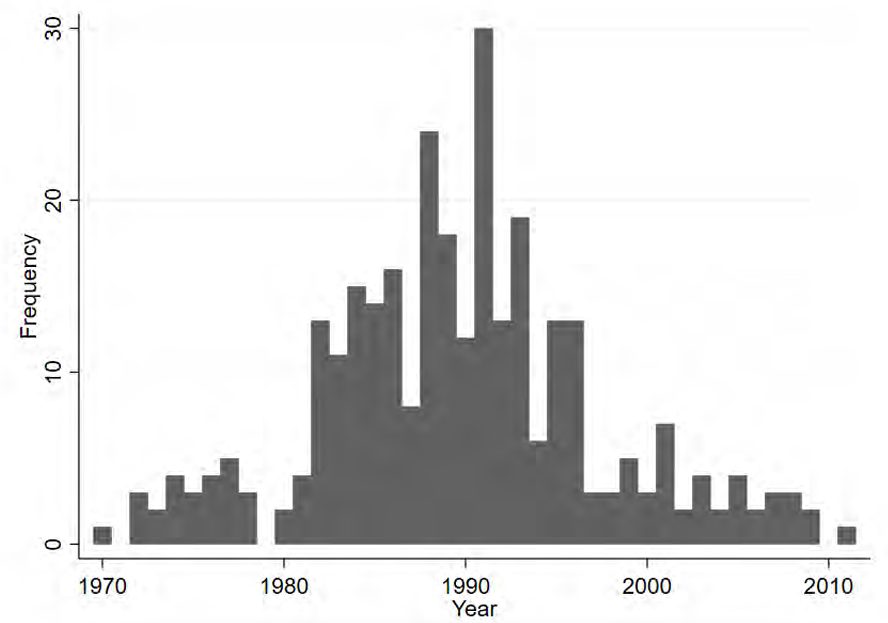
Note: This figure shows the approval years of at-large to ward reforms reported in the 1981-2011 ICMA Municipal Form of Government surveys. Because the 1986 wave asks only if a reform was approved between 1981-1986 and does not specify the exact year, reforms reported in this wave are randomly allocated to a year between 1981 and 1986 in the figure in order to prevent an artificial peak in 1986.

Figure A.2. Long-Run Trends in Housing Units Permitted

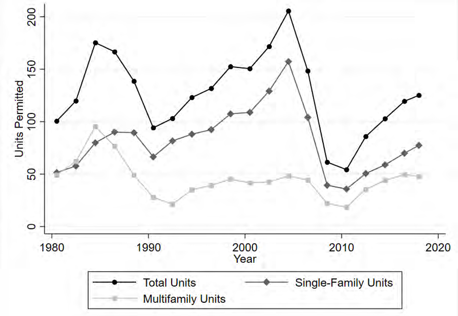
Note: This figure shows the number of housing units permitted in the average town in the analysis sample in each year of the Census Building Permits data.

Figure A.3. Event Study for LIHTC Units

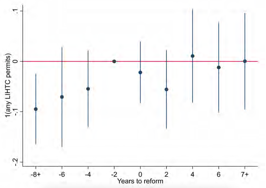
Note: This figure shows event study coefficients from the estimation of Equation 1 with 1(LIHTC permits) as the dependent variable. Year 0 is the year that a town approved a switch from at-large to ward elections. The dummies for years to treatment are bundled into two-year bins, and the label on the x-axis represents the later year. The specification includes town fixed effects and county-year fixed effects, and errors are clustered at the state level.

Figure A.4. Event Study for Total Units Permitted (Treated Towns)

Note: This figure shows event study coefficients from the estimation of Equation 1 with log(total units + 1) as the dependent variable. Year 0 is the year that a town approved a switch from at-large to ward elections. The dummies for years to treatment are bundled into two-year bins, and the label on the x-axis represents the later year. The specification includes town fixed effects and state-year fixed effects, and errors are clustered at the state level. Only towns that switch from at-large to ward voting during the sample period are included.

Figure A.5. Event Study for Single- and Multi-Family Units Permitted (Treated Towns)

Note: This figure shows event study coefficients from two separate estimations of Equation 1, with log(single-family units + 1) and log(multi-family units + 1) as the dependent variables. Year 0 is the year that a town approved a switch from at-large to ward elections. The dummies for years to treatment are bundled into two-year bins, and the label on the x-axis represents the later year. The specification includes town fixed effects and state-year fixed effects, and errors are clustered at the state level. Only towns that switch from at-large to ward voting during the sample period are included.

Figure A.6. Event Study for Total Units Permitted (Matched Sample)

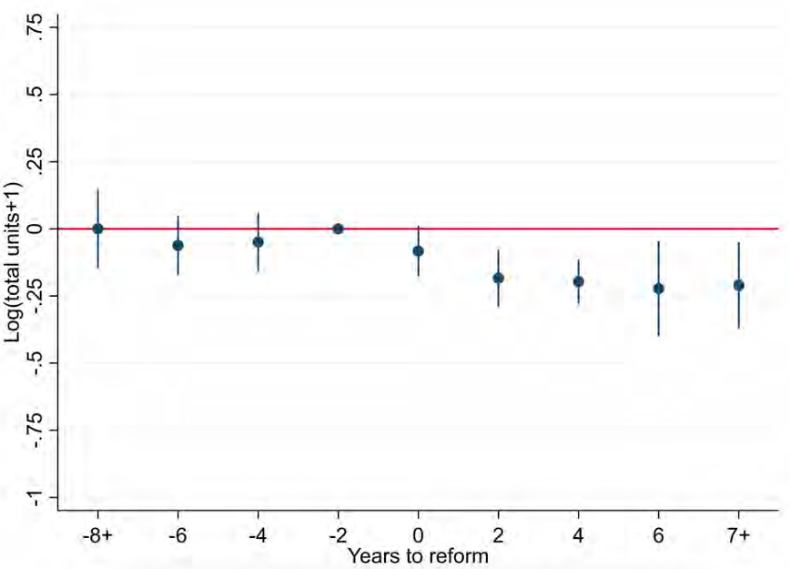
Note: This figure shows event study coefficients from the estimation of Equation 1 with log(total units + 1) as the dependent variable. Year 0 is the year that a town approved a switch from at-large to ward elections. The dummies for years to treatment are bundled into two-year bins, and the label on the x-axis represents the later year. The specification includes town fixed effects and state-year fixed effects, and errors are clustered at the state level. Only treated towns and towns in the matched sample are included.

Figure A.7. Event Study for Single- and Multi-Family Units Permitted (Matched Sample)

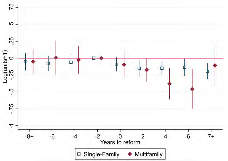
Note: This figure shows event study coefficients from two separate estimations of Equation 1, with log(single-family units + 1) and log(multi-family units + 1) as the dependent variables. Year 0 is the year that a town approved a switch from at-large to ward elections. The dummies for years to treatment are bundled into two-year bins, and the label on the x-axis represents the later year. The specification includes town fixed effects and state-year fixed effects, and errors are clustered at the state level. Only treated towns and towns in the matched sample are included.

Figure A.8. Event Studies for Early and Late Adopters

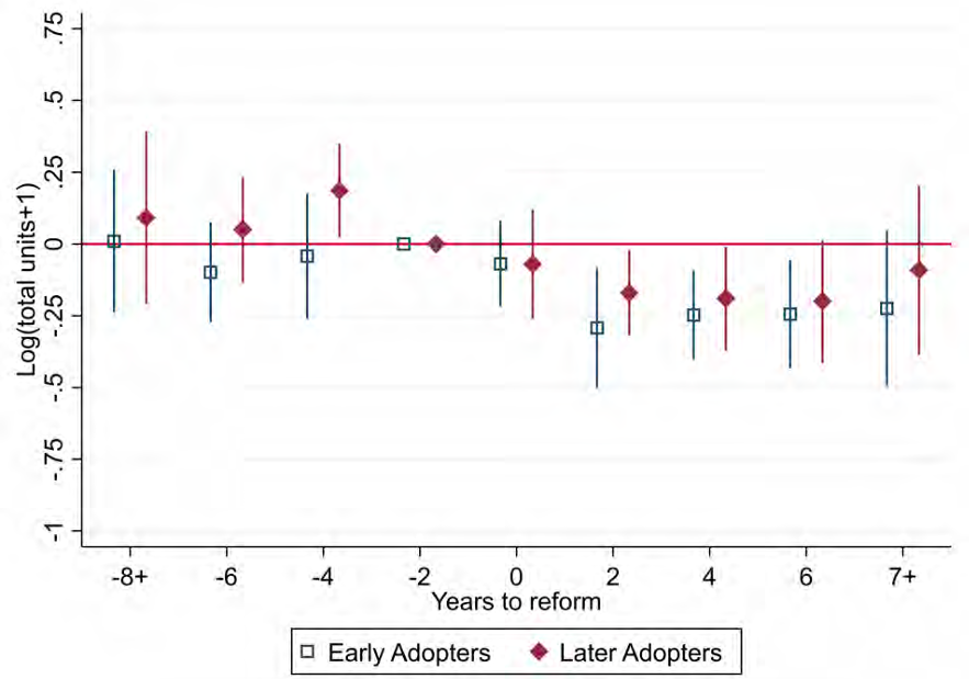
Note: This figure shows event study coefficients from two separate estimations of Equation 1. The coefficients labeled Early Adopters are from an estimation including only towns that reformed prior to 1995 in the treatment group. The Late Adopters estimation includes only towns that reformed after 1986. The specifications are otherwise identical to the baseline.

Table A.1. Characteristics of Treatment and Control Towns in 1980

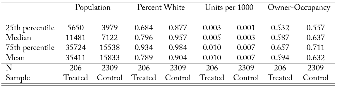
Note: This table shows the 1980 characteristics of those towns that switched from at-large to ward voting after 1980.

Table A.2. Robustness of Difference-in-Differences Estimates

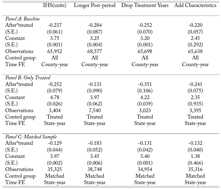
Note: This table repeats the baseline difference-in-differences estimation for total units permitted with four tweaks to the specification. Column 1 uses the inverse hyperbolic sine of total units instead of log(total units + 1). Column 2 drops the restriction on the number of post-reform years included in the specification. Column 3 drops the year the reform was approved and the previous year. Column 4 adds time-varying town characteristics (population, percent owner occupied, and percent white) as control variables.

Table A.3. Alternative Treatment Definitions

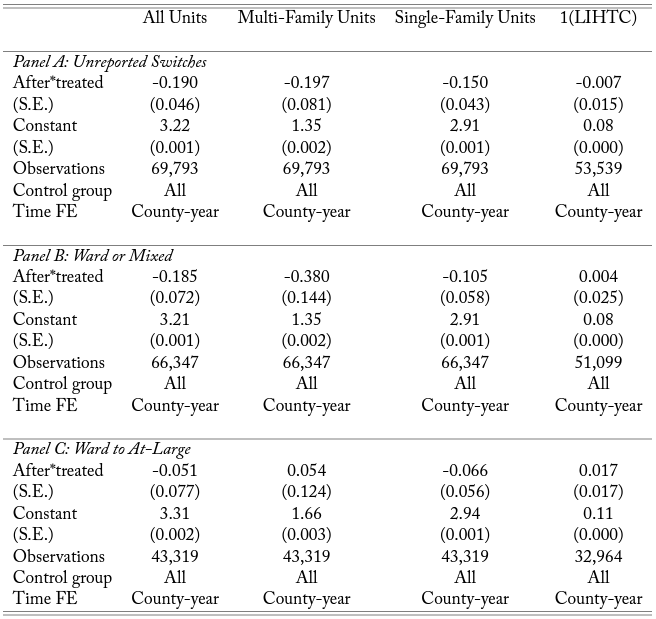
Note: This table shows results from alternative treatment definitions. Panel A expends the treatment definition to include towns that report an at-large council in one survey wave and a ward in the next (setting the treatment year to the midpoint of the gap between the two survey years). Panel B includes towns that report switching from at-large to mixed voting, as well as the baseline treated towns that report switching from at-large to purely ward voting. Finally, Panel C defines the treatment as reporting a ward system in one wave and an at-large in the next, again setting the treatment year to the midpoint of the two waves.

Table A.4. Effect of Reforms on Other Town Characteristics

Note: This figure repeats the baseline difference-in-differences specifications using town characteristics as the dependent variables. Because characteristics are only observed in decennial census years, only those years are included in the sample.

References

Abraham, S. and Sun, L. (2019). Estimating dynamic treatment effects in event studies with heterogeneous treatment effects. Working paper.

Albouy, D., Ehrlich, G., and Liu, Y. (2016). Housing demand, cost-of-living inequality, and the affordability crisis. NBER Working Paper #22816.

Baum-Snow, N. and Marion, J. (2009). The effects of low income housing tax credit developments on neighborhoods. Journal of Public Economics, 93(5):654–666.

Callaway, B. and Sant’Anna, P. (2019). Difference-in-differences with multiple time periods. Working paper.

Clark, A. and Krebs, T. (2012). Elections and policy responsiveness. In The Oxford Handbook of Urban Politics, The Oxford Handbook of Urban Politics. Cambridge University Press.

Clingermayer, J. (1994). Electoral representation, zoning politics, and the exclusion of group homes.
Political Research Quarterly, 47(4):969–984.

Davidson, C. and Korbel, G. (1981). At-large elections and minority-group representation: A re-examination of historical and contemporary evidence. Journal of Politics, 43(4):982–1005.

de Chaisemartin, C. and d’Haultfoeuille, X. (2019). Two-way fixed effects estimators with heterogeneous treatment effects. Technical report, National Bureau of Economic Research.

Diamond, R. and McQuade, T. (2019). Who wants affordable housing in their backyard? An equilibrium analysis of low income property development. Journal of Political Economy, 127(3).

Duranton, G. and Puga, D. (2019). Urban growth and its aggregate implications. Technical report, National Bureau of Economic Research.

Einstein, K., Palmer, M., and Glick, D. (2019). Who participates in local government? Evidence from meeting minutes. Perspectives on Politics, 17(1):28–46.

Elmendorf, C. S. (2019). Beyond the double veto: Housing plans as preemptive intergovernmental compacts. Hastings Law Journal, 71(1).

Engstrom, R. L. and McDonald, M. D. (1981). The election of blacks to city councils: Clarifying the impact of electoral arrangements on the seats/population relationship. American Political Science Review, 75(2):344–354.

Feinerman, E., Finkelshtain, I., and Kan, I. (2004). On a political solution to the NIMBY conflict.
American Economic Review, 94(6):369–381.

Feiock, R., Tavares, A., and Lubell, M. (2008). Policy instrument choices for growth management and land use regulation. Policy Studies Journal, 36(3):461–480.

Fischel, W. (2001). The Homevoter Hypothesis. Harvard University Press.

Freddie Mac (2018). The major challenge of inadequate U.S. housing supply. Technical report.

Frey, B., Oberholzer-Gee, F., and Eichenberger, R. (1996). The old lady visits your backyard: A tale of morals and markets. Journal of Political Economy, 104(6):1297–1313.

Glaeser, E. and Ward, B. (2009). The causes and consequences of land use regulation: Evidence from Greater Boston. Journal of Urban Economics, 65(3):265–278.

Goodman-Bacon, A. (2018). Difference-in-differences with variation in treatment timing. NBER Working Paper #25018.

Gyourko, J. and Molloy, R. (2015). Regulation and housing supply. In Duranton, G., Henderson, J. V., and Strange, W. C., editors, Handbook of Regional and Urban Economics, volume 5 of Handbook of Regional and Urban Economics, pages 1289–1337. Elsevier.

Hankinson, M. (2018). When do renters behave like homeowners? High rent, price anxiety, and NIMBYism. American Political Science Review, 112(3):473–493.

Hankinson, M. and Magazinnik, A. (2019). How electoral institutions shape the efficiency and equity of distributive policy. Working paper.

Hsieh, C.-T. and Moretti, E. (2019). Housing constraints and spatial misallocation. American Economic Journal: Macroeconomics, 11(2):1–39.

Ihlanfeldt, K. (2007). The effect of land use regulation on housing and land prices. Journal of Urban Economics, 61(3):420–435.

Leal, D. L., Martinez-Ebers, V., and Meier, K. J. (2004). The politics of latino education: The biases of at-large elections. Journal of Politics, 66(4):1224–1244.

Levinson, A. (1999). NIMBY taxes matter: The case of state hazardous waste disposal taxes. Journal of Public Economics, 74(1):31–51.

Lubell, M., Feiock, R., and Ramirez De La Cruz, R. (2009). Local institutions and the politics of urban growth. American Journal of Political Science, 53(3):649–665.

Parkhomenko, A. (2018). The rise of housing supply regulation in the U.S.: Local causes and aggregate implications. (275).

Pollakowski, H. O. and Wachter, S. M. (1990). The effects of land-use constraints on housing prices. Land Economics, 66(3):315–324.

Quigley, J. M. and Raphael, S. (2004). Is housing unaffordable? Why isn’t it more affordable? Journal of Economic Perspectives, 18(1):191–214.

Schleicher, D. (2013). City unplanning. Yale Law Journal, 122.

Schmidheiny, K. and Siegloch, S. (2019). On event study designs and distributed-lag models: Equivalence, generalization and practical implications. CEPR Discussion Paper No. DP13477.

Tausanovitch, C. and Warshaw, C. (2014). Representation in municipal government. American Political Science Review, 108(3):605–641.

Trebbi, F., Aghion, P., and Alesina, A. (2008). Electoral rules and minority representation in U.S. cities.
Quarterly Journal of Economics, 123(1):325–357.

Trounstine, J. (2010). Representation and accountability in cities. Annual Review of Political Science, 13:407–423.

Warding Off Development: Local Control, Housing Supply, and NIMBYs

Executive Summary

Resources

Focuses

Federal Agencies

Introduction