

1 Introduction
“The Ordinance was passed to ensure that residential rental housing remains available to long-term tenants, and because short-term rentals have undesirable impacts that threaten the stability and character of the City’s neighborhoods and result in increased rents.”
David Martin (2018), Santa Monica, California Director of Planning and Community Development
Driven by the emergence of online platforms such as Airbnb and Vacation Rentals by Owner (VRBO), short-term rentals (STRs) in the housing market have experienced significant global growth over the past decade.1An STR is typically defined as the rental of a fully furnished housing unit for a period ranging between one night and several months. In contrast, long-term rentals generally involve leases with a term of at least one year. By reducing information costs, these markets enable mutually beneficial transactions between property owners and transient visitors, and thus increase the utilization of (and economic surplus created by) housing capacity. Given that they increase certain neighborhood amenities (Basuroy et al., 2020) and the option value of home-ownership, STRs have the potential to increase housing prices (Horn and Merante, 2017; Garcia-López et al., 2020). Criticism of STR platforms has focused mostly on this price effect: higher housing prices means that long-term renters may be increasingly priced out of communities where they have lived for years (Nieuwland and van Melik, 2020).2Furthermore, given that homes account for roughly a quarter of aggregate household net wealth, movements in housing prices can have first-order consequences for household balance sheets (Stupak, 2019). As a consequence, there is an active policy debate surrounding STR regulation with an emphasis on restricting STRs on both the extensive (i.e., whether STRs are allowed in a given area) and intensive (i.e., what rules STR hosts must follow) margins.
Our contribution to this debate is an assessment of a simple point implied by the quote from a policymaker featured above: the net effect of STRs on housing prices is ambiguous due to the relationship between STRs and local amenities.3Throughout the paper, amenities are defined as “location-specific consumption goods.” STRs represent an extension of the capital stock available to the hospitality industry.
However, while the presence of hotels in a neighborhood creates positive demand spillovers for other service industries, hotels and other tourism-related firms are also associated with local negative externalities such as public intoxication, petty theft, and other “nuisances” (Brunt and Hambly, 1999; Ho et al., 2009). Insofar as STRs offer services that can substitute for the services of traditional hospitality firms—as has been proposed by Zervas et al. (2017) and Farronato and Fradkin (2018)—STRs may generate similar negative externalities. Airbnb, in particular, has received negative media attention for its “party house” listings (Lieber, 2015; Coles et al., 2017).4By offering “owner-absent” rentals of detached homes, STRs may host activities with negative externalities that would likely be deterred by the presence of hotel staff. Furthermore, as STRs are generally located in quieter, traditionally owner-occupied residential areas, the same activities may generate greater social costs when they take place in an STR as opposed to a hotel. Indeed, Fontana (2021) finds that increases in Airbnb penetration in London leads to increases in complaints against tourists and a decrease in neighborhood quality. If the cost of such externalities outweighs the benefits from increased demand for local businesses—in other words, if STRs sufficiently “threaten the stability and character” of neighborhoods (Martin, 2018)—the net effect of STRs on the overall level of local amenities, and potentially on housing prices, may be negative. In this paper, we demonstrate this both theoretically and empirically.
We formalize this idea in Section 3 with a partial equilibrium model of the housing market that builds on the work of Barron et al. (2020). In our model, home-owners choose between occupying their home themselves and listing it as a short-term rental. Having this option increases the value of owning housing. Our contribution is to consider the idea that STRs may also impose both positive and negative externalities on their neighbors. In equilibrium, an increase in the STR rental rate may reduce housing prices if the net effect of STRs on amenities for owner-occupiers in the neighborhood is sufficiently negative to outweigh the effect of the increased surplus earned by absentee landlords. Similarly, an exogenous change in the number of STRs in a given neighborhood may result in an increase or a decrease in housing prices, depending on the net impact of STRs on aggregate amenities and disamenities in that neighborhood.
To provide empirical evidence for the implications of our model, we turn to Los Angeles (LA) County, California. This area has one of the highest levels of amenities in the United States (Albouy, 2016) but also features a high degree of income and amenity inequality across its various communities (Bobo et al., 2000; Wolch et al., 2005; Charles, 2006). As we describe in Section 4, we employ data on individual housing prices from Zillow, data on Airbnb participation for individual dwellings from web scrapes, and crime data from local governments. We begin our analysis in Section 5 by considering the relationship between Airbnb listings and housing prices at the zip-code level. As our model makes clear, the number of Airbnb listings is endogenous so we employ an instrument based on the level of local amenities in each zip code prior to the entry of Airbnb into the regional housing market. We first estimate the relationship for Los Angeles County in the aggregate and find a positive effect mirroring other results in the literature (Barron et al., 2020). We then estimate the relationship for each city in LA County and find significant heterogeneity. For example, in the City of Los Angeles, a 1% increase in the number of Airbnb listings in a zip code is estimated to increase housing prices by 0.23%, but in Burbank, a higher-income, lower-density community, the same increase in listings is estimated to decrease housing prices by 0.11%.
These results suggest that regulations restricting STRs may lead to increased housing prices. In Section 6, we examine the effects of an STR restriction enacted by the wealthy oceanfront suburb of Santa Monica—a jurisdiction for which we estimate a negative relationship between STRs and housing prices. The 2015 law, enacted in part due to concerns about increasing housing prices in the city, was arguably the strictest regulation on STR activity in effect in the United States at the time (Sanders, 2015). It is important to note, upfront, that we are not claiming this policy change is exogenous to housing prices—per the contemporaneous press, it was implemented in response to a simultaneous increase in STR listings and housing prices (Logan, 2015). We first document that the law was (at least temporarily) successful in reducing the number of Airbnb listings that would be most likely to generate negative externalities. Using a difference-in-differences framework with the rest of LA County as a control, we show that these regulations almost certainly did not decrease housing prices and may have increased housing prices by about 8%. Finally, we provide suggestive evidence for our externality mechanism by examining detailed call data from the Santa Monica Police Department. Using a difference-in-differences framework with linear trends to account for delays in enforcement, we show that public intoxication calls decreased relative to other types of calls.5In a conference paper, Han and Wang (2019) study the relationship between STRs and the crime rate in New York City and San Francisco using policy changes that primarily affected commercial listings and find qualitatively similar results.
Our work contributes to the recent literature examining the relationship between STR markets and housing prices. Relative to this literature, which we broadly characterize as providing average effects of STRs, our work focuses on heterogeneity in the effects of STRs. Within this literature, the closest work to our own is that of Barron et al. (2020) who introduce the instrument described above and use it to estimate the average effect of Airbnb listings on housing prices across the U.S.—their result is similar to our estimate for LA County as a whole. In contrast, we extend their model and focus our empirical work on a particular geography to demonstrate significant heterogeneity. In a recent working paper, Filippas and Horton (2020) develop a model of home-sharing through subletting, focused on tenants and landlords with negative externalities, and using New York City (NYC) as an empirical setting. Calder-Wang (2019) estimates the distributional impacts from Airbnb in NYC and finds the losses to renters (via increased prices) exceed the gains to the hosts (via an increased option value of housing). Relative to this work, we allow for the possibility that STRs generate both positive and negative externalities and explore the impact of an STR regulation directly. Valentin (2021) examines the impact of STR regulation in New Orleans and finds that regulating and restricting STRs are associated with a decline in property values. In another working paper, Fonseca (2019) analyzes the immediate impact of Santa Monica’s law on long-term rental prices using a synthetic control approach, and finds little effect. In addition to our different focus on the effects of STRs on local amenities, we use data on home-ownership prices over a longer period to identify the effects of the law.
We also contribute to the growing literature examining the relationship between STRs and other hospitality firms, such as hotels and motels. By arguing that Airbnb listings are associated with negative externalities similar to those created by hotels, our work is complementary to other studies cited above which identify STRs as substitutes for traditional hotels. More broadly, our work contributes to the literature examining the relationship between various local externalities and housing prices (see e.g. Nelson, 1978; Bartik and Smith, 1987; Glaeser et al., 2001) as well as the effects of local policies on housing prices (see e.g. Friedman and Stigler, 1946; Pollakowski and Wachter, 1990; Glaeser and Luttmer, 2003; Glaeser et al., 2005; Diamond et al., 2019).
Our work further contributes to a broader literature examining the externalities of peer-to-peer markets. Within the transport sector, the rapid expansion of ridesharing apps such as Uber has led to increases in net restaurant creation, by providing restaurant patrons with easier access to previously inaccessible locations (Gorback, 2020). However, there have been added social costs associated with the growth of ridesharing, such as increases in the number of motor vehicle fatalities as well as increases in congestion and road use (Barrios et al., 2020). Understanding the net impact of peer-to-peer markets is essential in determining whether and how to regulate these nascent industries. We conclude in Section 7 with a discussion of these externalities and suggestions for both policymakers and future researchers.
2 Background
Our analyses operate at the intersection of private housing and hospitality markets, taking advantage of the long-standing heterogeneity between the various communities of Los Angeles County. In this section, we briefly describe this heterogeneity, provide a short history of STRs and Airbnb, and discuss the specific Santa Monica legislation ordinance restricting STRs.
2.1 Los Angeles County
Los Angeles County, with a population of more than ten million, is the single most populous county in the United States. According to the Bureau of Economic Analysis and the Census Bureau, LA county as a whole had a GDP of more than $700 billion and a median household income of $62,978 in 2016. The county is divided into 88 incorporated cities and 76 unincorporated areas with significant and sustained heterogeneity (Bobo et al., 2000).
Table 1 illustrates some of this heterogeneity in terms of median income, local characteristics, and median rents for LA County overall and for the City of LA and nine other notable cities within the county. See Appendix Figure A.1 for a map of these cities within LA County. Median income in the City of LA is slightly lower than the county as a whole, given that communities such as Malibu and Beverly Hills have median incomes more than twice that for the county as a whole. Malibu, a western beachside community, has a population density of only 353 residents per square mile, whereas the more centrally located West Hollywood has 13,359 residents per square mile. Public parks and dining opportunities vary widely as well—while the City of LA features 9.9 park acres per thousand residents, Pasadena offers only 2.5 park acres per thousand residents. Santa Monica offers 4.7 restaurants per thousand residents, while Pomona, on the far eastern border of the county, offers merely 1.3.
Table 1. Characteristics for Selected Cities in Los Angeles County
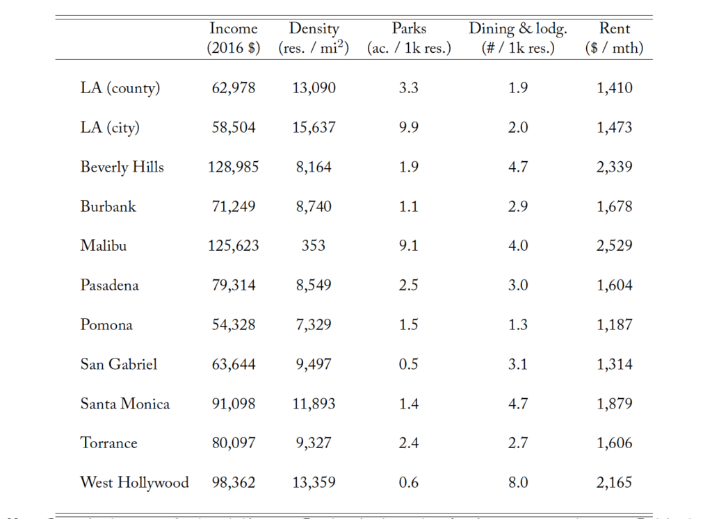
Notes: ‘Income’ is the 2016 median household income. ‘Population’ is the number of residents per square mile in 2010. ‘Parks’ is the number of acres of city parks per 1,000 residents in 2016. ‘Dining & lodg.’ is the number of establishments in NAICS category 72 per 1,000 residents in 2010. ‘Rent’ is the median gross rent in 2016 for renter-occupied housing with two bedrooms. All statistics from the Census Bureau except for parks, which is from the 2016 Los Angeles Countywide Comprehensive Park and Recreation Needs Assessment.
These differences in observable amenities are likely related to the differences in average rental rates for two-bedroom apartments, which in 2016 ranged from $1,187 in Pomona to over $2,500 in Malibu. Los Angeles currently ranks as the least affordable city in America, according to the Housing Opportunity Index (HOI) sponsored by the National Association of Home Builders and Wells Fargo.6https://www.nahb.org/News-and-Economics/Housing-Economics/Indices/Housing-Opportunity-Index The HOI for a community measures the share of homes sold that would have been affordable to median-income earners. During the fourth quarter of 2019, the HOI indicated that only 11.3% of homes sold in Los Angeles were affordable at a median income of $73,100. Population growth, rising income inequality, and supply-side constraints contribute to the Los Angeles metro area having the lowest home-ownership rate out of all major metropolitan areas (Ong et al., 2015).
2.2 Home sharing and the rise of Airbnb
“Home-sharing” gained popularity in the U.S. in the 1950s, as vacation rentals—in which visitors have private and exclusive (i.e., without the presence of a long-term resident) use of a housing unit for some period—became a viable alternative to hotels. These rental units were traditionally located in areas that expected and welcomed frequent turnover of travelers as well as the accompanying economic benefits of tourism. Launched in 1995, Vacation Rentals by Owner (VRBO) provided the first online platform for vacation or STR bookings; Booking.com entered a year later. These peer-to-peer markets connected travelers with vacation rental properties that were managed by their owners and allowed the booking of short stays (i.e., 30 days or fewer). As the “sharing economy” grew, so too did the number and diversity of neighborhoods in which travelers could find these “owner-absent” bookings.
Founded in 2008, Airbnb expanded the STR market by providing hosts a platform through which they could offer single rooms in their occupied homes, which gave travelers more options for lodging in residential neighborhoods. While these “owner-present” STRs differ substantially from traditional owner-absent vacation rental offerings (or hotel offerings), they quickly grew in popularity as a cheaper alternative. This in turn exposed new consumers to the possibility of owner-absent rentals. Today, Airbnb’s peer-to-peer market offers both owner-absent and owner-present options and lists more rooms than the largest six hotel groups combined (Airbnb, 2019).7couchsurfing.com offered owner-present STRs earlier than Airbnb, though their offerings are aimed at lower-income consumers and they do not offer owner-absent STRs.
2.3 Regulating STRs
Neither California nor the U.S. federal government explicitly regulates STRs—though we discuss the interaction of federal communications laws and local regulations below. Instead, STRs are regulated through local ordinances. In Section 6, we focus on Santa Monica’s Ordinance 2484CCS, which was adopted by its City Council on May 12, 2015. According to staff reports and the text of the measure, the city was roused to action because STRs removed “needed permanent housing from the market” and transient visitors could “disrupt the quietude … of the neighborhoods and adversely impact the community” (City of Santa Monica, 2019). The measure nominally banned owner-absent STRs, while allowing owner-present STRs to continue with additional licensing, reporting, and taxation requirements.
The ordinance was debated in the months before passage and was an outgrowth of a longer-term process by the City Council to update Santa Monica’s land-use and transportation plan that began in December 2013 and continued for several months beyond the adoption of the short-term rental regulation (Martin, 2015). This “spin-off ” ordinance was not unique—the City Council of Santa Monica passed other spin-off ordinances as a result of this process, including ordinances related to discrimination in long-term rental housing, water conservation policy, and commercial fitness instruction. None of these ordinances were directly related to land-use, building codes, or other regulations with first-order impacts on residential housing prices or neighborhood amenities. Furthermore, none of the ordinances passed during this period were directly related to establishments offering on-premise alcohol consumption or public intoxication, which we investigate in Section 6.1. The major components of the ongoing planning effort primarily concerned requirements for commercial buildings and multi-family dwellings, and thus it is unlikely that this process alone would have created significant changes in housing prices until its provisions went into effect and future construction projects were designed in compliance with those provisions. If anything, the land-use plan encouraged the construction of additional multi-family dwellings by rezoning certain areas in the city and easing restrictions on accessory dwelling units, which would decrease housing prices compared to a counterfactual with no change in land-use policy, even if such changes were anticipated.8The conclusions in this paragraph are drawn from our review of the text of the ordinance and contemporaneous measures as well as meeting minutes and archived video of Santa Monica City Council meetings. We are unable to find any evidence to contradict these assertions.
When the ordinance went into effect in June of 2015, Airbnb (among other platforms) quickly launched a legal challenge which made enforcement difficult (Dolan, 2019). The city had no ability to prevent landlords from honoring reservations made before the ordinance went into effect. Landlords worked to circumvent the provisions of the ordinance, finding ways to offer owner-absent STRs that complied with the rules. These circumventions included modifications to listings that likely decreased the probability that renters would generate externalities. For example, the owner may be present for a short period at the beginning and end of the rental period, or be occupying an adjacent dwelling. These actions resulted in several additional legal challenges.9See Diane Hayek v. City of Santa Monica, Los Angeles Superior Court No. 17STLC02007 (May 30, 2018); Diane Hayek v. City of Santa Monica, Los Angeles Superior Court No. BS170950 (August 19, 2019). Ultimately, the city prevailed in all cases.
Santa Moncia’s difficulty in enforcing their STR restriction is particularly relevant to our analyses given the results of Fontana (2021), who, using data from London, finds that “negative externalities can be explained by a lack of monitoring and co-ordination by [Airbnb] hosts”. If these legal challenges allowed absentee landlords to maintain STR listings without modification for a period, or at least to satisfy bookings made prior to the passage of the ordinance, any negative externalities generated by those listings are likely to be unaffected as well. Therefore our prior is that changes to the number (or composition) of listings and subsequent changes in negative externalities and house prices may be delayed or gradual. We return to these issues when we analyze police calls in Section 6.
Such regulatory and enforcement challenges have played out in similar ways around the country as local governments attempt to regulate STRs (Martineau, 2019). These challenges are often driven by Section 230 of the federal Communications Decency Act (CDA). Broadly construed, CDA 230 protects online platforms from responsibility for content posted by users. STR platforms have successfully used CDA 230 to challenge local regulations which require platforms to participate in the filtering of illegal listings.10Indeed, according to the Ninth Circuit ruling, Santa Monica won largely by constructing its measure in such a way that STR platforms were responsible only for collecting taxes and regulatory information, not removing content. HomeAway.com, Inc. v. City of Santa Monica, Ninth Circuit Court of Appeals No. 18-55367 (March 13, 2019). These challenges, combined with other perceived abuses of CDA 230 by other platforms, have led to various proposals for reform through legislation or regulation (Neuburger, 2020).
3 A model of housing with type-of-use externalities
To understand the potentially heterogeneous effects of STRs on housing prices and provide stylized intuition for our empirical work, we introduce a partial equilibrium model of housing choice that extends the work of Barron et al. (2020) by adding type-of-use externalities. Our goal is not to generate “sharp” falsifiable predictions—rather in the context of a literature which has both a) estimated that STRs generate increases in average housing prices (Barron et al., 2020) and b) documented significant negative externalities in particular local jurisdictions (Fontana, 2021), we show that the effect of STRs on equilibrium jurisdiction-level housing prices is ambiguous even in a parsimonious framework. Thus we abstract from several considerations (including long-term rentals and the ownership of multiple dwelling units) which do not affect the primary mechanism: the interplay between externalities and the option value (to home-owners) of offering STRs.
The model environment consists of a finite number of jurisdictions  , indexed by
  . Each jurisdiction offers a fixed quantity of housing
  . The total number of agents in the housing market is exogenous and given by
  . Each agent
  jointly decides in which jurisdiction to purchase a home and their usage of that home, i.e., whether to be an owner-occupier or an absentee landlord. We normalize to zero the utility of not entering the market.11For simplicity, we do not explicitly model long-term rental arrangements. The mechanism described here operates similarly in a model with long-term renters as long as those renters are affected similarly to owner-occupiers by location-specific amenities.
The utility derived by individual from owning and occupying housing in jurisdiction is

In this equation,  is a function that maps three jurisdiction-specific features into a scalar amenity value. The feature
  is a fixed, time-invariant amenity level that is unrelated to short-term rentals.
  is an increasing function that maps the level of STRs in jurisdiction to the level of positive amenities associated with STRs (such as extra restaurants), and
  is an increasing function that maps the level of STRs to the level of \textit{negative} amenities associated with STRs (such as crime).
  is the price of housing in jurisdiction and
  is an idiosyncratic preference shock.
With a slight abuse of notation, we assume that  is positive for all
  ,
,  and
and  and that
  is negative for all , and . We make no explicit assumption about second derivatives—though we note that, in general, one might expect increases in to affect and differently, i.e., negative externalities may be “worse” if the jurisdiction is “nicer.” As a consequence, the effect of an increase in STRs on jurisdictional amenity values is ambiguous, as can be seen through the partial derivative
(1) 
Jurisdictions with different levels of amenities (and therefore different levels of  and
and  ) and/or different levels of (and therefore different levels of and ) may therefore confer either greater or lesser utility when the level of STRs increases.
The utility an agent receives from being an absentee landlord is given by

where  is the sum of net STR revenues in jurisdiction net of any rental expenses and
  is the common discount rate.12We assume for simplicity there is no uncertainty in future per-period net revenues. We assume for simplicity $R_j$ is exogenous.13As STRs compete with other hospitality firms having large numbers of units, the effect of a small change in the number of STR units available in a particular jurisdiction on is likely to be second-order.
Also for simplicity, assume  (where
  ) is i.i.d. and follows a Type-I extreme value distribution. This implies that the probability (or choice share)
  of an individual choosing jurisdiction and usage-type is given by the familiar logit form

where  . In equilibrium, markets must clear:
  for all . Using this market-clearing condition, we can write the equilibrium price for houses in location (see Appendix A.1. for details):
(2) 
where  and
and  is the equilibrium number of short-term rentals in jurisdiction . We use the equilibrium housing price expression to derive an expression that guides the interaction between short-term rentals and housing prices. Our key insight comes from the relationship between the equilibrium price, the STR rental rate, and the number of STRs:
  and
and  :
:
(3) 
Equation (3) illustrates how a change in net discounted STR rental revenues impacts equilibrium home prices. Equation (4) provides the direct impact of STR listings on equilibrium housing prices. Note that  —the number of STRs always increases as the present value of STR revenue increases. However, the sign of and may vary. varies with the sign of
  —the net effect of STRs on residential amenities. For , there are three non-trivial cases to consider. For clarity of exposition, consider the effect of an increase in on the equilibrium price
  .
.
Case 1.  : STRs create net-positive amenities. In this case, as the number of STRs increases, the value of owner-occupied homes will increase, increasing demand for owner-occupation. Thus, equilibrium housing prices increase:
  .
.
Case 2.  and
and  : STRs create net-negative amenities and the magnitude of the change in the marginal benefit to absentee landlords exceeds the magnitude of the change in marginal benefit to owner-occupiers. In this case, increasing decreases amenities, but that decrease is not fully offset by the increased value realized by absentee-landlords and thus an increase in leads to a net increase in the demand for houses and the equilibrium housing price increases: .
Case 3. and  : STRs create net-negative amenities and the decrease in the marginal benefit to owner-occupiers exceeds the increase in the marginal benefit to absentee landlords. Here, while the increase in increases demand by absentee landlords, the increased number of STRs decreases demand by owner-occupiers by a greater amount. Thus, the net effect on demand for housing is negative and
  .
.
Equations (3) and (4) can be used to frame the expected impacts of STR regulations. Some STR regulations (e.g., occupancy taxes or other hospitality business taxes) may be viewed as a change to the present value of being an absentee landlord. Other regulations however may be direct shocks to the number of Airbnb listings allowed—e.g, limits on individual choices to be absentee landlords—resulting in a direct change in  .
.
4 Data
To explore the main implication of our model—that the relationship between STRs and housing prices is ambiguous—we collect data on housing prices, Airbnb listings, and crime reports from LA County. We choose this geography in part due to the long-term presence of Airbnb in the area. Any short-term extensive-margin competitive effects of entry are thus likely to have occurred before the period of our analyses. LA County also offers a distinct policy change in Santa Monica, but not elsewhere in the county.
Our data on housing prices is the Zillow Home Value Index (ZHVI), which we obtain from Zillow.com for the interval 1996–2019. The ZHVI reports the estimated median home value at the zip-code-month level, adjusted for seasonality. To construct the ZHVI, Zillow estimates the sale price for all homes in each zip code based on recent sales in that area (Bruce, 2014). The ZHVI has previously been used to study a variety of issues in housing markets, including land-use regulations (Huang and Tang, 2012), strategic responses to mortgage modification programs (Mayer et al., 2014), and credit market shocks (Greenstone et al., 2020).
We obtain Airbnb listing data from insideairbnb.com and tomslee.net, where each of these sources provides snapshots of consumer-facing listings available on specific days, collected by web-scraping. For each listing, we observe a unique host and room identifier, the jurisdiction for the short-term rental unit, the daily price, and the (mutually exclusive) room type: “Entire unit,” “private room,” and “shared room.” We aggregate these listings to the zip-code level and construct measures of STR supply based on the total number of listings of each type. These data were scraped at irregular intervals (see Appendix Section A.3 for more details). We obtain all scrape dates from 2014 (the earliest available) to 2019. These data have previously been used to understand the relationship between Airbnb listings and housing prices in other geographies (Garcia-López et al., 2020). Finally, to construct the instrumental variable described in Section 5, we obtain Google Trends data for “Airbnb,” and also collect the number of food and accommodation establishments (NAICS 72) in each zip code in 2010 from the ZIP Code Business Patterns data released by the U.S. Census.
Table 2 reports summary statistics for these data as used in our analyses. We discuss the details of our sample construction procedure in Appendix Section A.3. The first set of rows reports the ZHVI for LA County as a whole and for the set of its constituent cities displayed in Table 1. The last column computes the average annual percentage change in each ZHVI between 2014 and 2019. Each city experienced increases in housing prices throughout our data. However, these increases range from 5% in Torrance to 15% in Beverly Hills.
The City of LA experienced an increase of 7%, while prices in Santa Monica increased by 11%. The second set of rows reports counts of Airbnb listings by type and jurisdiction. Again, every area experienced considerable growth throughout the period we study. However, Santa Monica experienced the only year-over-year decline of listings in the dataset: entire unit listings (which are generally owner-absent) decreased from 606 in 2015 to 450 in 2016 as the Santa Monica STR regulation was passed, went into effect, and was increasingly enforced. However, as STR suppliers in Santa Monica adjusted to the new regulations, the number of listings slowly increased—by 2019, the number of “entire unit” listings exceeded the pre-regulation count, though per our discussion in Section 2, the efforts of listers to comply with Santa Monica’s regulations means these listings likely generated externalities at lower rates.
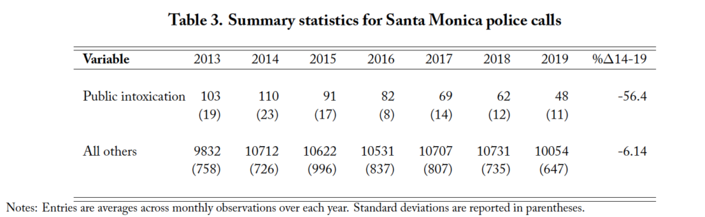
To provide descriptive evidence of the relationship between STRs and negative externalities, we collect data on police calls from the Santa Monica Open Data Project for 2013–2019.14https://data.smgov.net/Public-Safety/Police-Calls-for-Service/ia9m-wspt For each call, we observe the date and time, the location of the caller, and the reason for the call. Importantly, these data encode the reason for the call at a much finer level of detail than is used for either the Uniform Crime Reporting data or National Incident-Based Reporting System data compiled by the Federal Bureau of Investigation. Unfortunately, few cities in the U.S. report data at this level of detail and none do so at the same frequency; we are not aware of any cities that report data that can be harmonized with the Santa Monica data for direct comparison.15For example, Eugene, Oregon, reports call reasons with high granularity, but uses catgories with different definitions and aggregates to the annual level. We focus on comparing calls for which the reason listed includes ‘public intoxication,” against other calls because public intoxication frequently appears in media reports in media reports about the nuisance effects of STRs (Lieber, 2015; Griffith, 2020). In Appendix A.8, we explore other call types. Table 3 reports summary statistics for these complaint data. After (generally) initial increases, the number of each type of call declined over our study period. The total number of calls we consider decreased 33% from 2013 to 2019.
Table 2. Summary statistics for housing prices and Airbnb listing data
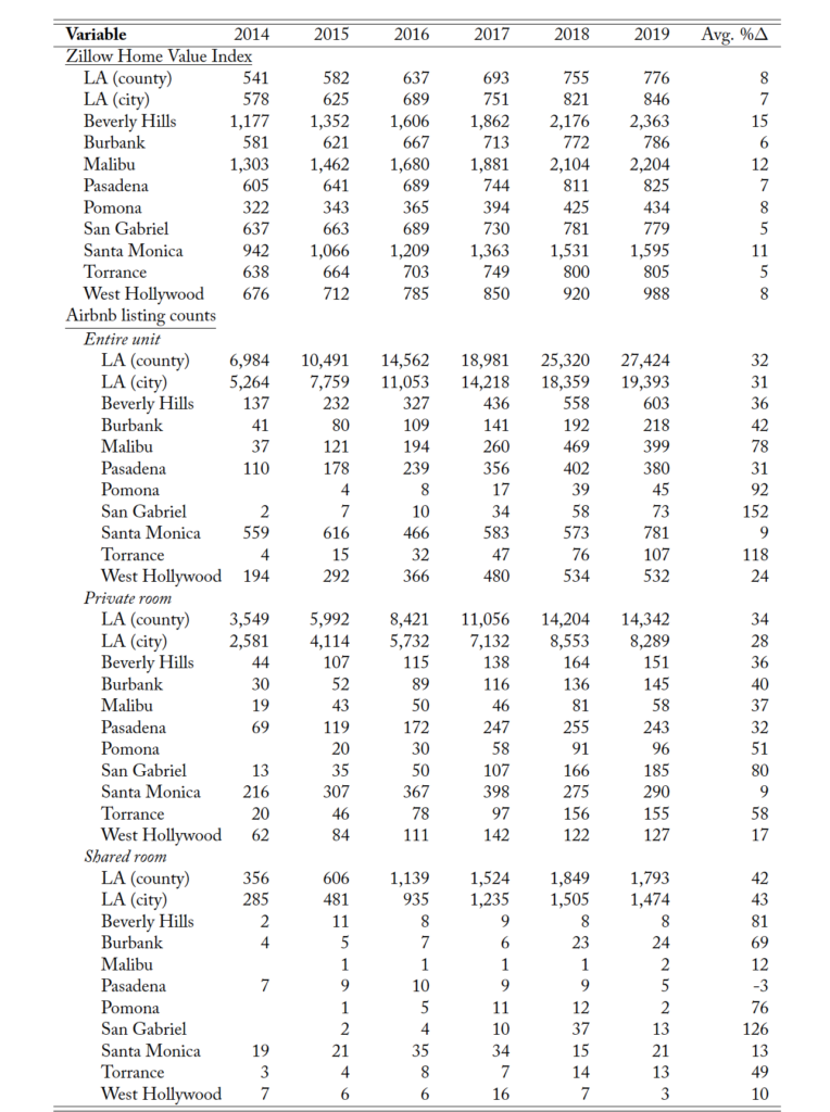
Notes: Entries are averages across monthly observations during each year. The Zillow Home Value Index is measured in thousands of dollars and reflects the median home value in the given jurisdiction in each year as estimated by Zillow.
5 Evidence of heterogeneous impacts of STRs on housing prices
Equation (4) suggests a testable hypothesis: at the margin, the relationship between STRs and housing prices may be positive or negative.16The null hypothesis is that the relationship between STRs and housing prices is weakly positive. In this section, we test this hypothesis by estimating the effects of Airbnb listings on local housing prices. Although our data contains the current per-night price of each listing, we focus on Equation (4) as opposed to Equation (3) for two reasons. First, our data represent a noisy estimate of Rj —while the lifetime expected revenue for an STR is correlated with an observed per-night price, reservations, and future prices (and therefore the time series of revenues) is unknown. Second, the observed listings represent a selected sample—we do not observe STR pricing for housing units that are not listed. As listings and housing prices are both equilibrium outcomes, we proceed by following an instrumental variable strategy in conjunction with fixed effects.
Let ZHVIjct be the Zillow Home Value Index for zip code z in jurisdiction j at year-month time t. Equation (4) suggests the following estimating equation:
(4) 
where  is the number of Airbnb listings, ϵzjt is an unobservable, and FX is a set of fixed effects.17In practice, a small number of observations have zero listings. We therefore use log(1 + ). Our results are qualitatively robust to dropping these observations. The coefficients of interest are {β1j}, which vary across neighborhoods.18In other words, we estimate Equation (5) by interacting the log of the number of listings with city indicators. To control for jurisdiction-level characteristics that stay constant over time and are correlated with both Airbnb listings and housing prices, we include geography-based fixed effects. While zip-code fixed effects are an obvious option, zip codes in LA county are generally coterminal with city boundaries, and therefore zip-code fixed effects would preclude identification of β1j . We cannot use city fixed effects for the same reason. Therefore, we turn to area code fixed effects. There are 11 area codes in LA County, each covering a geographically contiguous area with boundaries that (generally) do not overlap with city boundaries. Appendix Figure A.2 illustrates these area code boundaries along with city boundaries. While these areas were not designed to be completely homogeneous, their geographic continuity ensures at least some correlation between the jurisdictions within their scope. For example, area code 310 includes the entire coastline of LA County across several cities. We also include year fixed effects to account for time-varying characteristics that are correlated with both Airbnb listings and housing prices, such as population growth and macroeconomic conditions.19As the ZHVI is seasonally adjusted, month-of-year fixed effects are not necessary.
Despite these fixed effects, there may be some component of  which is correlated with . Therefore, we employ the instrument proposed by Barron et al. (2020). We interact the Google Trends measure for the search term “airbnb” with the number of establishments in the food services and accommodations industry (NAICS 72) in each zip code in the base year of 2010—prior to large-scale Airbnb entry in the area. Specifically, if
  is the Google Trends measure and
  is the number of NAICS 72 establishments in 2010 in zip code , our instrument is

Our identifying assumption is that ![E[z_{zjt}\cdot \epsilon_{zjt}] = 0](https://www.thecgo.org/wp-content/ql-cache/quicklatex.com-2f5b7165cf9d078aa3d6003b65681f31_l3.svg "Rendered by QuickLaTeX.com") . Intuitively, acts as a proxy for the degree to which a given neighborhood attracts tourists over the long term (and therefore may be a more attractive place for entry by a potential Airbnb host). On its own, however, this variable is likely also to be correlated with housing prices, because food service establishments are probably positive neighborhood amenities (Meltzer and Schuetz, 2012). The variable scales this “touristy-ness” measure by the overall market size for Airbnb. Given that the attractiveness of restaurants in a specific neighborhood to long-term residents (or prospective residents) of that neighborhood is likely not correlated with the nationwide market presence of Airbnb (as measured by Google Trends), the interaction between these two variables will likely satisfy the exclusion restriction. Furthermore, this instrument is correlated with housing prices in a given period only insofar as it is correlated with the number of Airbnb listings, conditional on the included fixed effects.20One may be concerned that spillovers are not contained to the area-code level. To the extent that STRs are substitutes for hotels, public intoxication incidents will likely occur near the location of the STR. We report summary information and first-stage estimates for our instrument in Appendix Section A.4.
. Intuitively, acts as a proxy for the degree to which a given neighborhood attracts tourists over the long term (and therefore may be a more attractive place for entry by a potential Airbnb host). On its own, however, this variable is likely also to be correlated with housing prices, because food service establishments are probably positive neighborhood amenities (Meltzer and Schuetz, 2012). The variable scales this “touristy-ness” measure by the overall market size for Airbnb. Given that the attractiveness of restaurants in a specific neighborhood to long-term residents (or prospective residents) of that neighborhood is likely not correlated with the nationwide market presence of Airbnb (as measured by Google Trends), the interaction between these two variables will likely satisfy the exclusion restriction. Furthermore, this instrument is correlated with housing prices in a given period only insofar as it is correlated with the number of Airbnb listings, conditional on the included fixed effects.20One may be concerned that spillovers are not contained to the area-code level. To the extent that STRs are substitutes for hotels, public intoxication incidents will likely occur near the location of the STR. We report summary information and first-stage estimates for our instrument in Appendix Section A.4.
Table 4 reports our estimates of  for the cities listed in Table 1. In Column (1), we report an estimate for the entire sample which includes every zip code in LA county with no fixed effects. In Column (2), we add fixed effects for the year and area code. While the key coefficient decreases relative to Column (1), it is still positive and significantly different from zero. We estimate that a 10% increase in Airbnb listings increases average house prices in LA County by 0.93%. These estimates are similar in magnitude to those reported by Barron et al. (2020), who report that a 10% increase in Airbnb listings leads to a 0.77% increase in house prices as measured by the ZHVI.21This estimate comes from the unconditional effect of ln(Airbnb Listings) on ln(ZHVI ) as reported in the first row of Table 6, Column (6) of Barron et al. (2020). Indeed, the reported confidence intervals overlap.
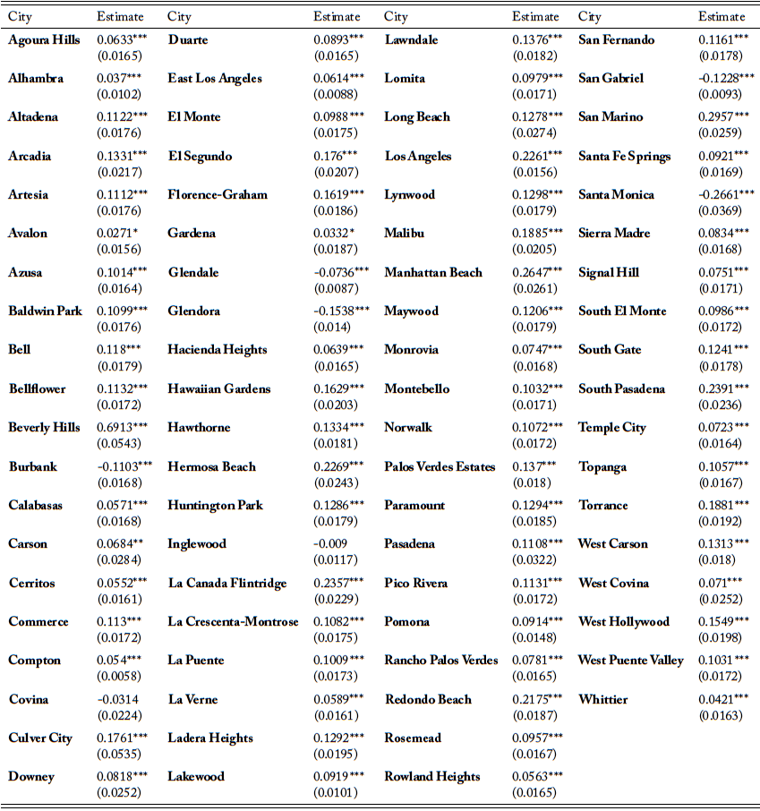
In Columns (3) through (6), we estimate individual coefficients for each city. In Column (3) we include no fixed effects, in Columns (4) and (5) we add first year and then area code fixed effects. Column (6) includes both sets of fixed effects and is our preferred specification. Appendix Table A.2 reports estimates for this specification for all cities. Across cities, the coefficients vary widely. In West Hollywood, a 10% increase in the number of Airbnb listings increases housing prices by 1.55%, whereas in Santa Monica, a 10% increase in the number of Airbnb listings decreases housing prices by 2.66%.
Figure 1. The Heterogeneous Effect of Airbnb Listings on Housing Prices
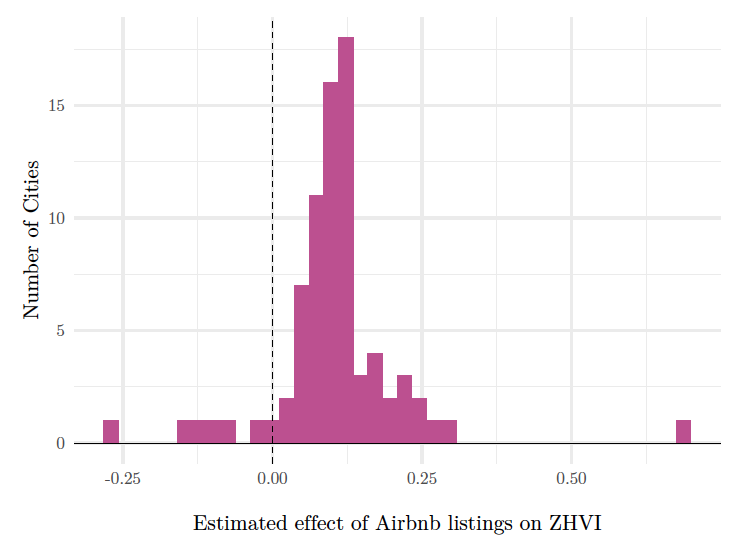
Notes: This figure depicts a histogram of the estimated s from Equation (5) for all cities. Estimates come from the fully saturated model: Column (6) in Table 4.
We have chosen to report estimates for these particular cities because they are more likely to be familiar to many readers. However, the estimated heterogeneity in the estimates of is similar across the entire set of estimates. Figure 1 depicts the distribution of the full set of coefficients for each jurisdiction using our fully saturated model. Of the 78 cities in our preferred specification, 7 have negative point estimates—5 of which are distinguishable from zero in the statistically significant sense.22We drop 14 cities which are collinear with our fixed effects: Acton, Castaic, Claremont, Diamond Bar, La Mirada, Lake Hughes, Lancaster, Littlerock, Monterey Park, Palmdale, San Dimas, Santa Clarita, Valyermo, and Walnut. We take these results as broadly consistent with the previous literature: for most jurisdictions, the estimated relationship between STR listings and housing prices is positive, just as the estimated relationship for the region as a whole is positive. However, the average effect for the region aggregates over a substantial degree of heterogeneity at the city level.
Our model does not make sharp predictions about the characteristics of neighborhoods that are more likely to have a negative relationship between STRs and housing prices—it suggests merely that in these locations, the net external effect of an STR is negative. Equation (1) implies that the relevant jurisidiction-level characteristics are the rates at which STRs change both positive and negative local amenities, and the rate at which those amenities translate into the utility of owner-occupation in the jurisdiction. This provides a scaffolding with which to frame a discussion of the different jurisdictions listed in Table 4.
Table 4. The Effect of STRs on Housing Prices for Selected Cities in LA County
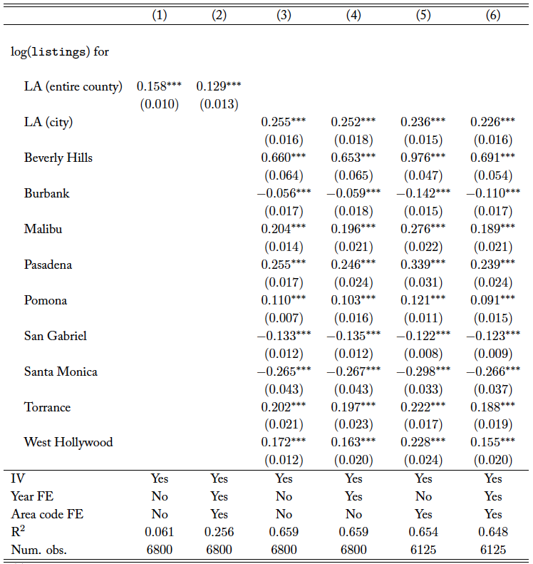
Notes: This table reports estimates of Equation (5). We estimate coefficients for each city in LA county; full estimates are available in Appendix Table A.2. An observation is a zip-code-month. The dependent variable is the log of the Zillow Home Value Index. listings is the number of Airbnb listings, which we instrument for with an interaction of Google Trends and the number of food establishments. First stage details are reported in Appendix Section A.4. Heteroskedastic-robust standard errors are in parentheses; we explore alternative clustering techniques in Appendix A.6. Stars indicate p values: ∗∗∗ p < 0.01; ∗∗ p < 0.05; ∗ p < 0.1. In Columns (5) and (6) we drop cities that are collinear with the area fixed effects.
The three cities with negative estimated coefficients are Burbank, San Gabriel, and Santa Monica. First, suppose that the rate at which amenities translate into utility is constant across jurisdictions. Burbank is adjacent (but not home) to Universal Studios Hollywood, a popular tourist attraction for adults aged 18 to 34 which sells alcohol (Glueck, 2016). If short-term renters are spending tourist dollars outside of Burbank and returning to their rental after an evening of alcohol consumption,  may be low and
  may be high. San Gabriel is adjacent to Pasadena, which hosts a number of notable events throughout the year, including the Rose Bowl Parade and Rose Bowl Game, both events associated with high alcohol consumption (Rose Bowl Community Prevention Council, 2013). Similarly to Burbank, if short-term renters of properties in San Gabriel spend their tourism dollars elsewhere, may be low and may be high. We note that Pasadena itself has a positive estimated coefficient. Even if is the same for both San Gabriel and Pasadena, if short-term renters of properties in Pasadena tend to spend their tourism dollars in Pasadena, for Pasadena will be higher than for San Gabriel, thus offsetting . Indeed, the estimated coefficient for Pasadena is significantly lower than the coefficient for Malibu and Beverly Hills, which do not have similar events. Finally, Santa Monica is the closest beach access for students of both the University of California, Los Angeles, and the University of Southern California. If local STRs allow students (and their guests) to imbibe more heavily, confident in the presence of local (private) lodgings, may be high while may be low. We investigate this externality channel for Santa Monica in Section 6.1.
It is also possible that the rate at which amenities translate into utility varies across jurisdictions. For example, we estimate a positive coefficient for Malibu, a beachside community 20 miles west of Santa Monica. Relative to Santa Monica, Malibu is considerably less dense, has fewer dining and lodging estabishments per-capita (see Table 1), and is further away from the downtown core of Los Angeles. As a consequence, negative externalities created by e.g. alcohol consumption are likely to be both less frequent due to the decreased access to relevant establishments, and less impactful to local residents, due to the greater distance between dwellings.
6 The effect of Santa Monicas STR regulation
The evidence of the previous section suggests that the marginal impact of additional STRs on housing prices in some areas can be negative. Our framework attributes the heterogeneity in the sign of the relationship to the channel of negative amenities (for owner-occupiers) generated by the presence of STRs. This suggests some further hypotheses. Suppose an area in which the marginal impact of STRs on housing prices is negative implements a policy that reduces the number of STRs, either through affecting or by decreasing  directly. Then we should expect to see both an increase in housing prices and a decrease in negative amenities.
We test these hypotheses by exploring the effects of Santa Monica’s STR restrictions by estimating the effect of the regulation on housing prices using a difference-in-differences approach at the zip-code level using the City of LA as a control. Contemporaneous media reports (and the text of the regulation itself ) make it clear that the regulation was passed in part as a response to rapidly rising housing prices and a lack of affordable long-term housing (both rental and owner-occupied) in Santa Monica. Thus we cannot claim that the policy represents a “clean” natural experiment. However, given that the stated goal of the policy was to decrease housing prices, any finding to the contrary provides evidence of the heterogeneous impacts of STRs. Our analysis of police report data then provides evidence for our proposed mechanism.
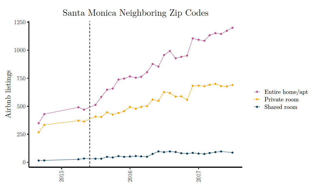
First, we document that the reform did in fact reduce the level of Airbnb listings in Santa Monica. Figure 2 illustrates the effect of Santa Monica’s STR regulation on Airbnb listings. Each point requires a separate web scrape. Only 4 scrapes were conducted before the policy was enacted, but subsequent scrapes occurred at roughly monthly intervals for the two years following the implementation of the regulation. While there is an enforcement lag, there is a clear drop in the number of “entire unit” listings after the reform, and no similar drop appears for the City of LA. The number of entire-home listings eventually rebounded to the pre-regulation level. As discussed in Section 2, this was in part due to ongoing changes in behavior and legal challenges by landlords, Airbnb itself, and the City of Santa Monica. Conversations with city officials indicate that the policy effectively changed the nature of entire-home listings to reduce those which may generate negative externalities, though verifying those claims is difficult due to the nature of the Airbnb data.
Figure 2. Airbnb listings by room type
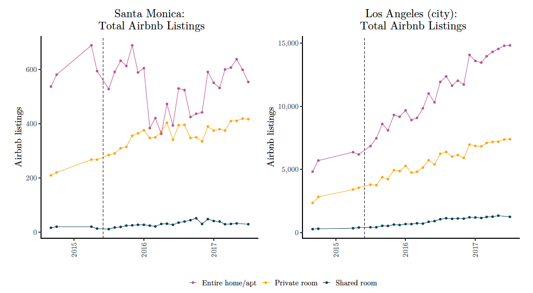
Notes: Each point on each graph represents a separate web scrape of Airbnb’s listings for that city. The dotted line represents May 2015, when Santa Monica’s ordinance was passed. Web scrape data was obtained from insideairbnb.com and tomslee.net and harmonized. See Section 4 for details.
Let  be the housing price (as measured by the ZHVI) for zip code at time
  . We estimate the parameters of
(5) 
where we define  as an indicator equal to one if the zip code falls in Santa Monica and zero otherwise (the City of LA), and
  as an indicator equal to one if the year-month is later than May of 2015 (when the policy was enacted). The coefficient on the interaction between these two terms (
 ) provides an estimate of the local average treatment effect. As before,
  are fixed effects for area code and year.
The parameter β3 is identified if the pre-treatment differences in the outcome variable are the same (parallel pre-trends), and if the treatment itself did not generate spillovers that affect the control groups (see, for example, Hansen et al., 2020). We note that Santa Monica rests at the western edge of LA County, and, per Table 2, the number of Airbnb listings within Santa Monica before the reform numbered approximately 1/16th of those in the City of Los Angeles. We thus conclude that it is unlikely that Santa Monica’s reform affected the number of STRs in the City of Los Angeles (and thus could have affected LA house prices through the STR channel).23In Appendix Figure A.3 we plot the time series of listings in zip codes immediately bordering Santa Monica. Though the number of observations prior to the reform is limited, significant spillovers are not apparent.
To evaluate the parallel pre-trend assumption, we plot the difference between Santa Monica and Los Angeles in the average of the log of housing prices over time, where the average is taken over the zip codes that comprise each city, in Figure 3. We begin our analysis in 2012, the “trough” of housing prices in the region in the wake of the Great Recession. The difference is relatively constant for several years prior to the reform, but increases starting in mid-2014 (in levels, both cities were experiencing increases in housing prices at this time). As the reform was discussed for some time before enactment, we interpret much of this movement as a potential anticipation effect.
Figure 3. Differences in housing prices between Santa Monica and Los Angeles
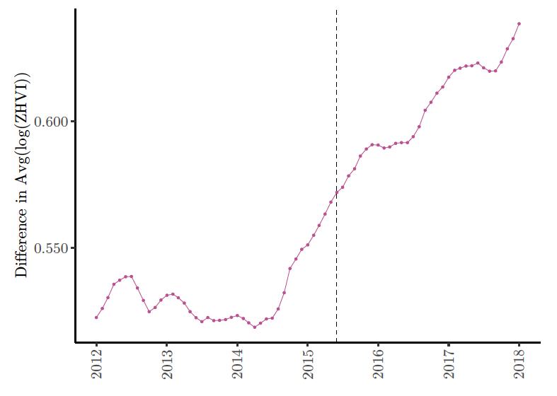
Notes: Data come from the Zillow House Value Index. Observations are the difference in the average log of housing prices between Santa Monica and Los Angeles, where the average is taken over the zip-code-month observations for each city. The date of the reform is shown by a vertical dashed line.
The top panel of Table 5 reports estimates of Equation (6) using a bandwidth of 36 months to avoid the effects of the Great Recession.24In an earlier draft of this paper, we used the optimal bandwidth technique of Imbens and Kalyanaraman (2011) to perform this
analysis, which suggested a longer bandwidth overlapping the Great Recession. In Column (1), we do not include fixed effects—in Column (2) we add area code fixed effects, and in Column (3) we add year fixed effects. The point estimates are statistically identical across all three specifications—we estimate that the reform increased housing prices in Santa Monica by 7.7% relative to a counterfactual of no reform. This estimate conforms to the estimates in the previous section; the reform decreased Airbnb listings in Santa Monica by approximately 15%, which per Table 4 should generate an increase in housing prices of approximately 4%.
In the bottom panel of Table 5, we perform a falsification test by altering the timing of the STR regulation to 24 months after the true date as a placebo reform. The point estimates are both smaller in magnitude than the estimates for the true reform and are imprecisely estimated. In Appendix Figure A.7, we show our results are largely robust to alternative bandwidth selection techniques in the literature. Though power is reduced, we can still conclude that the policy likely did not reduce housing prices.
Table 5. The effect of Santa Monica’s STR regulation on housing prices
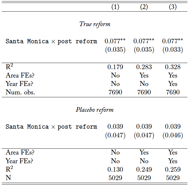
Notes: This table reports estimates of Equation (6) using a bandwidth of 36 months (see text for details). An observation is a zip-codemonth. The dependent variable is the log of the Zillow Home Value Index. Heteroskedastic-robust standard errors are in parentheses. Stars indicate p values: ∗∗∗ p < 0.01; ∗∗ p < 0.05; ∗ p < 0.1.
6.1 Exploring negative externalities in the form of police calls
Our framework suggests that the results in the previous section are driven by negative externalities generated by STRs. To evaluate this mechanism, we use a difference-in-differences approach to estimate the impact of STR regulations on public intoxication calls to police relative to other police calls in Santa Monica. Per Section 2, negotiations and legal maneuvers between STR listers and the City of Santa Monica resulted in gradual enforcement. We therefore add linear trend terms terms to the traditional difference-in-differences specification and model the log of the number of police calls of type  at time (where
  for the month when the policy when into effect) as
(6) ![\begin{equation*} \begin{split} \log(calls_{it}) = &\alpha_0 + \alpha_1 \times \texttt{intox}_i+ \alpha_2 \times \texttt{post}_t + \alpha_3 \times \texttt{intox}_i \times \texttt{post}_t \\ & + t \times [\alpha_4 + \alpha_5 \times \texttt{intox}_i+ \alpha_6 \times \texttt{post}_t + \alpha_7 \times \texttt{intox}_i \times \texttt{post}_t]\\ & + FX + \varepsilon_{it} \end{split} \end{equation*}](https://www.thecgo.org/wp-content/ql-cache/quicklatex.com-5b6929659b03f1525fa4d98a1ef6a75b_l3.svg "Rendered by QuickLaTeX.com")
where  is an indicator equal to one if the observation falls after the normalized policy date. We include month-of-year fixed effects to account for the seasonality of tourism.
Figure 4. Public intoxication and other police calls in Santa Monica
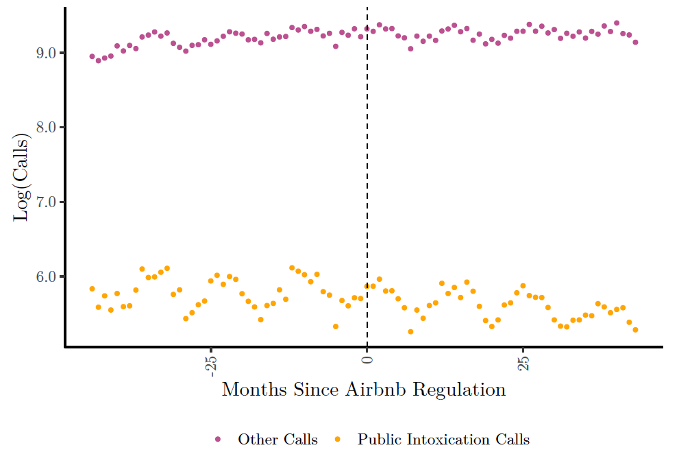
Figure 4 illustrates the log of the number of police calls in the public-intoxication category as well as all other calls. Table 6 reports our estimates of Equation (7). The relevant parameters are the level and time trend interaction terms for post × intox calls. Given the delay in enforcement mentioned in Section 2 and the fact that existing reservations were largely honored, it is perhaps unsurprising that there is no immediate discontinuity in police calls at the time the policy is enacted. However, post-reform, calls trend consistently downward. This effect is weaker, although more precisely estimated, when fixed effects are included. This trend persists for more than two years after the policy was enacted, despite the eventual increase in listings seen in Figure 2. As discussed in Section 2, negotiations and legal maneuvers between Airbnb listers and the City of Santa Monica resulted in post-reform listings that were qualitatively different and may have been less likely to generate public intoxication police calls. In Appendix A.8 we explore event studies for related call types.
Table 6. Difference-in-differences evidence of Santa Monica’s STR regulation effect on police calls for public intoxication
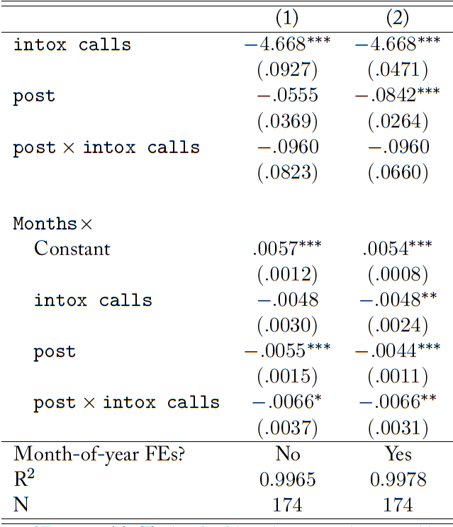
Notes: This table reports estimates of Equation (7). The bandwidth is chosen per the optimal bandwidth technique of Imbens and Kalyanaraman (2011). An observation is a month-call-type. The dependent variable is the log of the number of police calls reported in Santa Monica. Heteroskedastic-robust standard errors are in parentheses. Stars indicate p-values: *** p < 0.01; ** p < 0.05; * p < 0.1.
7 Conclusion
As the short-term rental (STR) housing market has expanded over the past several years, jurisdictions around the world have struggled to respond to its presence. Several media reports have captured policymakers’ concerns about the effect of STRs on long-term housing prices (e.g. Henley, 2019; Minder and Abdul, 2020). Other reports have focused on the deleterious effects of STRs on neighborhoods, particularly from the perspective of neighboring long-term residents (Griffith, 2020). These different stories are potentially contradictory—if STRs sufficiently reduce local amenities, their presence could be associated with lower, not higher, housing prices.
In this paper, we present a highly stylized model to demonstrate that STR listings at the intensive margin can reduce housing prices. Our model makes a simple point: since STRs can have both positive and negative impacts on local amenities, the impact of STRs on housing prices is an ambiguous function of the net effect of STRs on amenities—and therefore the effect of policies designed to curb STRs on housing prices is ambiguous as well. We illustrate this point empirically with both a panel analysis of the relationship between Airbnb listings and housing prices across jurisdictions within LA County, and a difference-in-differences analysis of Santa Monica’s housing prices before and after their 2015 regulation, using the City of LA as a control. In both analyses, we found evidence consistent with the hypotheses stemming from our model: STRs can lead to lower housing prices, and regulating them can increase housing prices. We provide evidence for our proposed mechanism in the form of an event study of calls to police in Santa Monica. We find that while the policy did not have a measurable immediate effect (likely due to enforcement lags), Santa Monica’s policy was associated with a decrease in the number of public intoxication police calls over time.
Our results have broad implications for housing policy. Many policymakers have focused on type-of-use regulations on housing units to restrict or ban STRs (Coles et al., 2017). These restrictions are expected to reduce the option value of owning a housing unit and therefore to decrease housing prices. However, in contrast to previous work, we show that such a policy may have the opposite effect. We provide a framework for thinking about why the effect might be positive or negative by separately considering the effect of STRs on positive and negative local amenities. In particular, the pattern of negative relationships between STR listings and housing prices may suggest that local policymakers may wish to focus their attention on STRs when short-term visitors are likely to spend their tourism dollars in other jurisdictions—bringing any negative externalities back to their temporary “home.” This conclusion, however, is based on ad hoc examinations of tourism in the particular jurisdictions within LA County—a qualitative exercise which would be challenging to translate to a quantifiable form that is broadly applicable across geographies. We leave it to future work to systematically and separately quantify the effects that STRs have on positive and negative amenities across jurisdictions.
These results also point to the importance of taking into account possible additional effects of peer-to-peer transaction platforms when considering regulation. Across industries, the literature consistently finds that peer-to-peer transactions increase surplus but tend to increase variance and/or risk relative to more traditional products and services. Examples include Uber (Barrios et al., 2020), Kickstarter (Mollick, 2014), Craigslist (Kroft and Pope, 2014), and Fiverr (Hannák et al., 2017). Furthermore, the provisions of the Communications Decency Act imply that these platforms have the potential to create outcomes which are biased along racial and gendered lines (Doleac and Stein, 2013; Edelman and Luca, 2014; Hannák et al., 2017). At the same time, the potentially positive externalities that these markets may generate imply that regulations may have unintended consequences (Cunningham et al., 2019). In the case of Airbnb and other short-term housing rental platforms, our results suggest that while federal policy may help ensure more uniform treatment for consumers, local decision-makers may be best-suited to set local policy for
residents.
Appendix
A.1 Equilibrium Housing Prices
In this section, we derive Equation2 —the equilibrium housing price equation. To simplify notation, we write  . Furthermore, define
  and
and  . Using the market clearing condition we can write:

A.2 Maps
In this section, we provide two maps to assist readers who may not be familiar with LA County. Figure A.1 illustrates the 88 incorporated cities in Los Angeles County. We highlight those which are displayed in Tables 1 and 4. Figure A.2 provides an overview of the area codes used as fixed effects and their intersection with cities in Los Angeles County.
Figure A.1. The cities of LA County
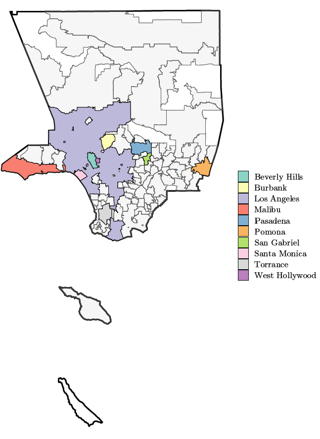
This figure depicts incorporated city boundaries in LA County. The highlighted cities are those displayed in Table 4. White areas within the county borders are unincorporated.
Figure A.2. The area codes of LA County
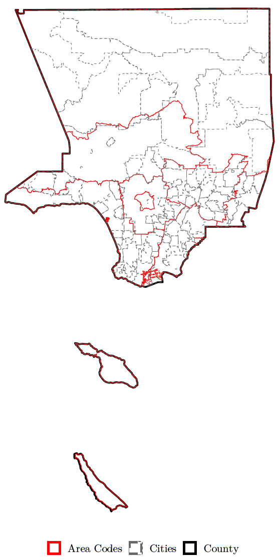
This figure overlays area codes on the city boundaries of LA county.
A.3 Sample Construction Details
In this section, we detail our sample construction procedure. Observations of house prices begin in 1996 and observations of police calls begin in 2006. Our Airbnb scrapes (from both sources) are collected at irregular intervals and date back to 2014. For all our estimates, we start with the full sample and select the estimation window via the optimal bandwidth technique of (Imbens and Kalyanaraman, 2011).
Since our data on Airbnb scrapes is more limited than the ZHVI data and the incidents call data, we restrict the estimation window for our city-level estimation of Equation (5). We merge the publicly available Tomslee and Inside Airbnb data to assemble the most comprehensive data possible. Each dataset contains a room id and scrape date variables. The room id variable is specific to an individually listed room.25The Inside Airbnb data contains a few year-months with multiple scrapes—such as November of 2019. Since we are ultimately interested in the number of listings at the zip-code year month level, we keep one room id per year month. After merging the Tomslee and Inside Airbnb data, we keep observations based on a unique room id and year-month pairing; which drops duplicate observations from both repeated scrapes within a month and observations that are shared by Tomslee and Inside Airbnb.
Both of our sources contain geo-coordinates of the listings. We intersect the listing locations with U.S. census ZTCA shapefiles and aggregate within zip codes and year-month to obtain total listings by zip-code-year-month. As demonstrated in Figure 2, before the policy, the scrapes are somewhat irregular. We thus restrict our estimation window from July 2015 to July 2017 as in this window, we have scrapes for each year-month. We then merge this data to the Zillow ZHVI data along with the instrument (which is constructed at the zip-code year-month level) to obtain our panel used to estimate Equation (5).
These coordinates are often listed with noise to maintain landlord privacy. Inside Airbnb notes that the noise-induced in these coordinates keeps the true coordinates within a 150m radius. Thus it is likely that some listings are recorded as located in zip-codes adjacent to their true zip code. We interpret this as adding classical measurement error to our sample, thus attenuating our estimates toward zero. However, for this reason (as well as the policy change in Santa Monica), it is possible that we may observe some spillovers between adjacent zip codes. In Figure A.3, we plot the number of Airbnb listings each month for zip codes immediately adjacent to Santa Monica. This graph follows the pattern displayed by the City of Los Angeles closely—and does not follow the pattern observed in Santa Monica—indicating that policy- or measurement-error-based spillovers are unlikely.
Figure A.3. Airbnb Listings in zip codes adjacent to Santa Monica
Notes: Each point on each graph represents a separate web scrape of Airbnb’s listings. The dotted line represents May 2015, when Santa Monica’s ordinance was passed. Web scrape data was obtained from insideairbnb.com and tomslee.net and harmonized.
A.4 Instrument Details
When estimating Equation (5), we instrument for the number of Airbnb listings by interacting the Google Trends index for the search term airbnb with the number of restaurants in a given zip code in 2010, before the widespread market growth of Airbnb. Figure A.4 displays Google Trends data at the monthly level from 2010 through 2019. Figure A.5 illustrates the distribution of zip codes in the U.S. according to the log of the per-capita number of food and accommodation establishments (as defined by NAICS 72). On the left graph, dots on the horizontal axis indicate the zip codes that comprise Santa Monica; the right graph illustrates the zip codes in the City of Los Angeles. While the density of restaurants in Santa Monica is clearly above the mean, the distribution of LA zip codes roughly matches the U.S. as a whole. Table A.1 reports first-stage estimates. Our instrument enters positively and significantly.
Figure A.4. Google Trends data used in instrument construction
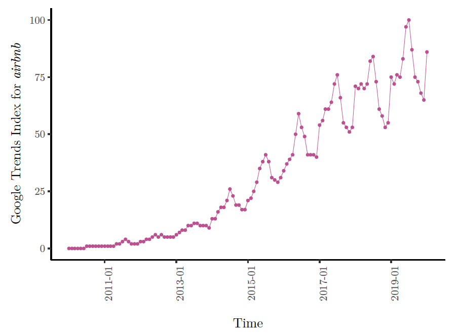
Figure A.5. Restaurant data used in instrument construction
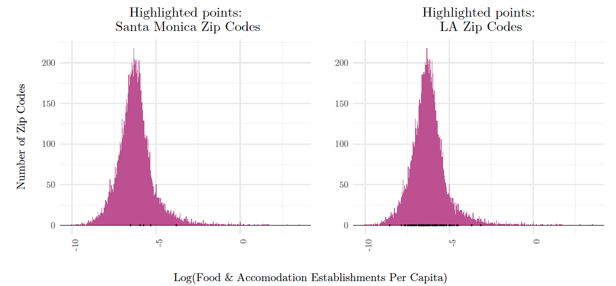
Notes: These figures illustrate the distribution of zip codes in the U.S. according to the log of the per-capita number of food and accomodation establishments in 2010 (as defined by NAICS 72). Dots on the horizontal axis indicate zip codes for the cities in question.
Table A.1. First-stage instrument results
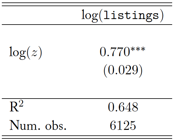
Notes: This table reports first-stage instrumental variables estimates of Equation (5). An observation is a zip-code-month. Heteroskedastic-robust standard errors are in parentheses. Additional parameters of Equation (5) are included, but not reported for space. Stars indicate p values: ∗∗∗ p < 0.01; ∗∗ p < 0.05; ∗ p < 0.1.
A.5 IV results for all cities
Table A.2. The relationship between Airbnb listings and housing prices for all cities in Los Angeles County
Notes: This table reports the full set of relevant coefficients for Column (6) of Table 4. An observation is a zip-code-month. Cities include both incorporated sub-county jurisdictions and unincorporated areas as defined by the U.S. Census. The dependent variable is the log of the Zillow Home Value Index. Heteroskedastic-robust standard errors are in parentheses. Stars indicate p values: ∗∗∗p < 0.01; ∗∗p < 0.05; ∗p < 0.1.
A.6 IV Results: Alternative Standard Error Clustering
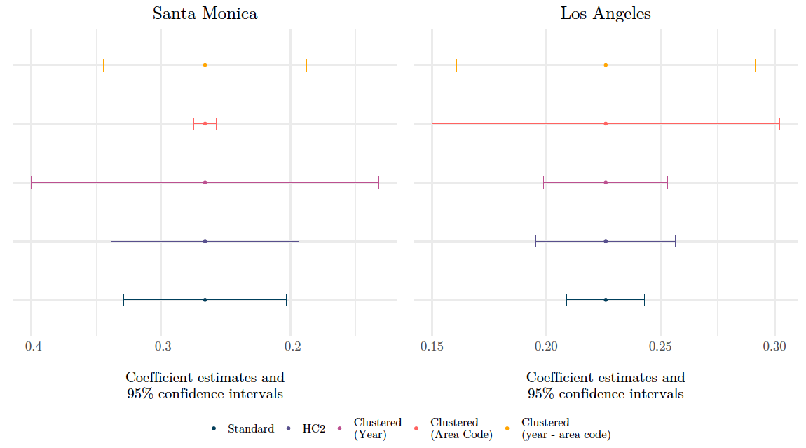
In this section, we present our primary IV estimates with alternative standard error clustering. Our estimates are remarkably robust to different standard error types. As a visual tool, we provide a coefficient plot for Santa Monica and LA, in which we vary the standard error type. We use our most saturated specification (with year and area code fixed effects) for each specification presented.
Figure A.6. Comparing standard errors under alternative clustering
A.7 Santa Monica’s STR Regulation: Other Optimal Bandwidth Techniques
In this section, we re-estimate our difference-in-differences specification that examines the effect of Santa Monica’s STR regulation on housing prices. In the main paper, we used a window of 36 months to avoid the influence of the Great Recession on housing prices. Here, we explore using the methods of Calonico et al. (2014), Ludwig and Miller (2007), and Imbens and Kalyanaraman (2011). The coefficient estimates are presented in Figure A.7 along with 95% confidence intervals. Note that using the selection method of CCT and CV, we cannot reject the null hypothesis that the effect of the policy was different than zero. Hence, we view our results as providing evidence that the policy may have increased housing prices—but more conservatively—could have also done nothing. In no specification do we find a reduction in housing prices from the policy.
Figure A.7. Alternative bandwidth techniques
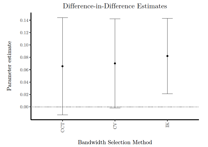
Notes: This figure illustrates point estimates and 95% confidence intervals for estimates of the effect of Santa Monica’s STR regulation on housing prices per Equation (6) using different bandwidth selection techniques. CCT refers to Calonico et al. (2014), CV refers to Ludwig and Miller (2007), and IK refers to Imbens and Kalyanaraman (2011).
A.8 Other police call types
In this section we explore trends in other types of police calls that may be generated by STR activity. We explore party complaints and noise complaints. For each of these, we estimate an event study (for comparison, we include a similar estimation for public intoxication calls). For call type in time we estimate the parameters of
(7) 
where  refer to month-of-year fixed effects.
The results are reported in Table A.3. We illustrate these estimates with the raw data in Figures A.8, A.9, and A.10.
Table A.3. Event study evidence of Santa Monica’s STR regulation effects on various police call types
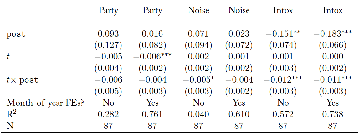
Notes: This table reports estimates of Equation (8). The bandwidth is chosen per the optimal bandwidth technique of Imbens and Kalyanaraman (2011). An observation is a month-year. The dependent variable is the log of the number of police calls reported in Santa Monica for one of three call types: party complaints, noise complaints, or public intoxication complaints. Heteroskedastic robust standard errors are in parentheses. Stars indicate p-values: *** p < 0.01; ** p < 0.05; * p < 0.1.
Figure A.8. Event study for party complaint incidents in Santa Monica
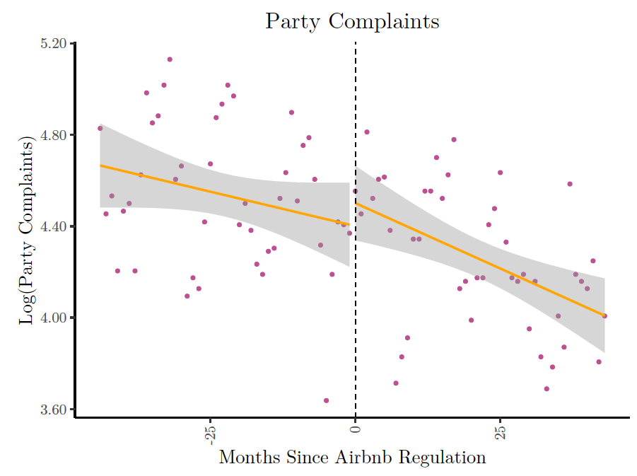
Figure A.9. Event study for loud music incidents in Santa Monica
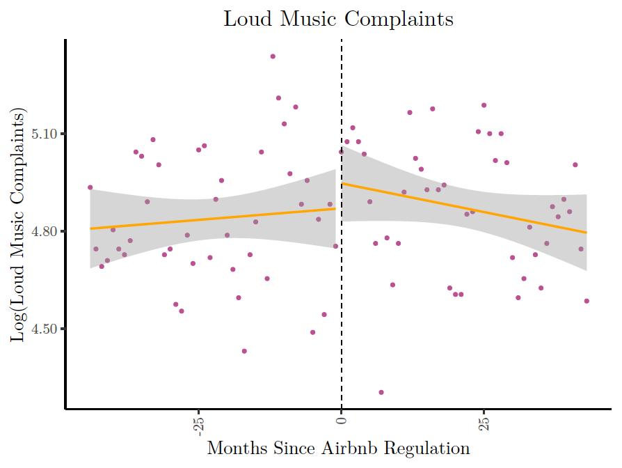
Figure A.10. Event study for public intoxication incidents in Santa Monica
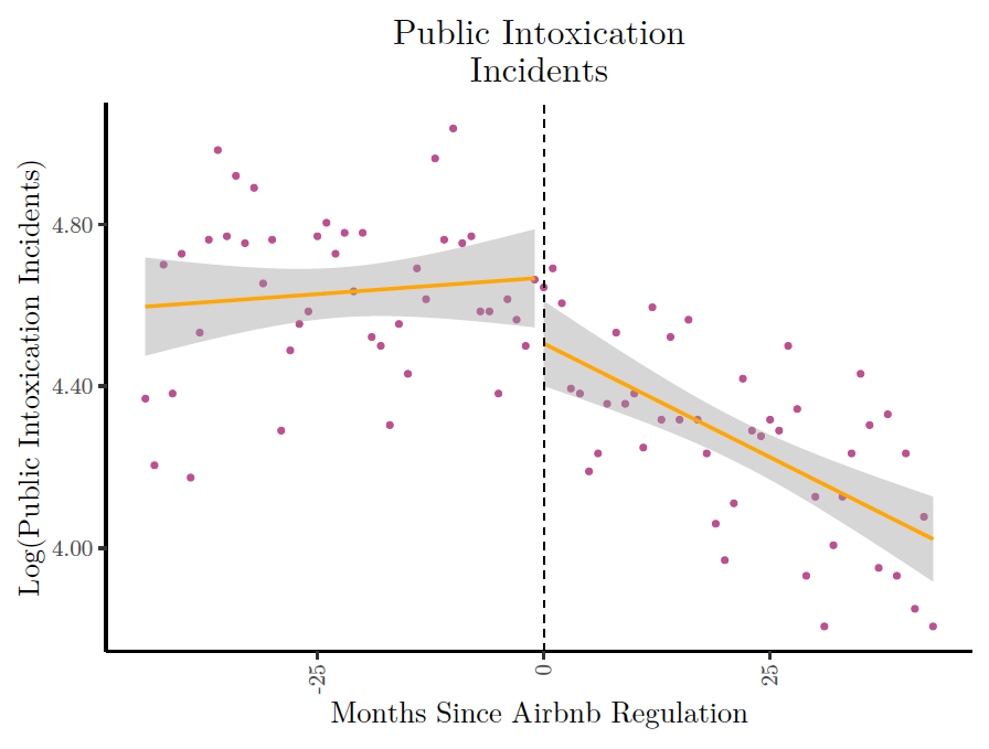
References
Airbnb (2019, March). Airbnb hosts shared more than six million listings around the world. https://news.airbnb.com/airbnb-hosts-share-more-than-six-million-listings-around-the-world/.
Albouy, D. (2016). What are cities worth? Land rents, local productivity, and the total value of amenities.Review of Economics and Statistics 98(3), 477–487.
Barrios, J., Y. Hochberg, and H. Yi (2020). The cost of convenience: Ridehailing and traffic fatalities. BFI Working Paper.
Barron, K., E. Kung, and D. Proserpio (2020). The effect of home-sharing on house prices and rents: Evidence from Airbnb. Marketing Science.
Bartik, T. J. and V. K. Smith (1987). Urban amenities and public policy. In Handbook of Regional and Urban Economics, Volume 2, pp. 1207–1254. Elsevier.
Basuroy, S., Y. Kim, and D. Proserpio (2020, 02). Sleeping with strangers: Estimating the impact of airbnb on the local economy.
Bobo, L. D., M. L. Oliver, J. J. H. Johnson, and V. Abel Jr (2000). Prismatic Metropolis: Inequality in Los Angeles. Russell Sage Foundation.
Bruce, A. (2014). Zillow Home Value Index: Methodology. Zillow Real Estate Research. Retrieved Aug 15, 2014.
Brunt, P. and Z. Hambly (1999, Apr). Tourism and crime: A research agenda. Crime Prevention and Community Safety 1(2), 25–36.
Calder-Wang, S. (2019). The distributional impact of the sharing economy on the housing market.
Calonico, S., M. D. Cattaneo, and R. Titiunik (2014). Robust nonparametric confidence intervals for regression-discontinuity designs. Econometrica 82(6), 2295–2326.
Charles, C. Z. (2006). Won’t You Be My Neighbor: Race, Class, and Residence in Los Angeles. Russell Sage Foundation.
City of Santa Monica (2019). Staff report 3778: Introduction and first reading of an ordinance amending chapter 6.20 to strengthen regulation of home-sharing. Technical report.
Coles, P. A., M. Egesdal, I. G. Ellen, X. Li, and A. Sundararajan (2017). Airbnb usage across New York City neighborhoods: Geographic patterns and regulatory implications. Forthcoming, Cambridge Handbook on the Law of the Sharing Economy.
Cunningham, S., G. DeAngelo, and J. Tripp (2019). Craigslist reduced violence against women. Technical report.
Diamond, R., T. McQuade, and F. Qian (2019). The effects of rent control expansion on tenants, landlords, and inequality: Evidence from San Francisco. American Economic Review 109(9), 3365–94.
Dolan, M. (2019, December). Santa Monica and Airbnb settle case after appeals court rules for city. Los Angeles Times.
Doleac, J. L. and L. C. Stein (2013). The visible hand: Race and online market outcomes. Economic Journal 123(572), F469–F492.
Edelman, B. G. and M. Luca (2014). Digital discrimination: The case of Airbnb.com. Harvard Business School NOM Unit Working Paper (14-054).
Farronato, C. and A. Fradkin (2018, February). The welfare effects of peer entry in the accommodation market: The case of Airbnb. Working Paper 24361, National Bureau of Economic Research.
Filippas, A. and J. J. Horton (2020). The tragedy of your upstairs neighbors: The externalities of home-sharing platforms.
Fonseca, C. C. (2019, June). The effects of short-term rental regulations: Evidence from the City of Santa Monica. Technical report.
Fontana, N. (2021). Backlash against Airbnb: Evidence from London. Technical report.
Friedman, M. and G. J. Stigler (1946). Roofs or Ceilings?: The Current Housing Problem. Foundation for Economic Education.
Garcia-López, M.-., J. Jofre-Monseny, R. Martínez-Mazza, and M. Segú (2020). Do short-term rental platforms affect housing markets? Evidence from Airbnb in Barcelona. Journal of Urban Economics 119, 103278.
Glaeser, E. L., J. Gyourko, and R. E. Saks (2005). Why have housing prices gone up? American Economic Review 95(2), 329–333.
Glaeser, E. L., J. Kolko, and A. Saiz (2001). Consumer city. Journal of Economic Geography 1(1), 27–50. Glaeser, E. L. and E. F. Luttmer (2003). The misallocation of housing under rent control. American Economic Review 93(4), 1027–1046.
Glueck, J. (2016). Millennials are spending more time at an unexpected location: Theme parks. Technical report.
Gorback, C. (2020). Your Uber has arrived: Ridesharing and the redistribution of economic activity.
Greenstone, M., A. Mas, and H.-L. Nguyen (2020, February). Do credit market shocks affect the real economy? Quasi-experimental evidence from the Great Recession and “normal” economic times. American Economic Journal: Economic Policy 12(1), 200–225.
Griffith, E. (2020, October). New York Times.
Han, W. and X. Wang (2019). Does home sharing impact crime rate? A tale of two cities. In ICIS 2019 Proceedings.
Hannák, A., C. Wagner, D. Garcia, A. Mislove, M. Strohmaier, and C. Wilson (2017). Bias in online freelance marketplaces: Evidence from taskrabbit and fiverr. In Proceedings of the 2017 ACM conference on computer supported cooperative work and social computing, pp. 1914–1933.
Hansen, B., K. Miller, and C. Weber (2020). Federalism, partial prohibition, and cross-border sales: Evidence from recreational marijuana. Journal of Public Economics 187, 104159.
Henley, J. (2019, June). Ten cities ask EU for help to fight Airbnb expansion. Guardian.
Ho, T., J. Zhao, and M. P. Brown (2009, Feb). Examining hotel crimes from police crime reports. Crime Prevention and Community Safety 11(1), 21–33.
Horn, K. and M. Merante (2017). Is home sharing driving up rents? Evidence from Airbnb in boston. Journal of Housing Economics 38(C), 14–24.
Huang, H. and Y. Tang (2012). Residential land use regulation and the US housing price cycle between 2000 and 2009. Journal of Urban Economics 71(1), 93–99.
Imbens, G. and K. Kalyanaraman (2011, 11). Optimal Bandwidth Choice for the Regression Discontinuity Estimator. Review of Economic Studies 79(3), 933–959.
Kroft, K. and D. G. Pope (2014). Does online search crowd out traditional search and improve matching efficiency? Evidence from Craigslist. Journal of Labor Economics 32(2), 259–303.
Lieber, R. (2015, October). New worry for home buyers: A party house next door. New York Times. Logan, T. (2015, April). Plan targets short-term rental units. Los Angeles Times, C1–C2.
Ludwig, J. and D. L. Miller (2007, 02). Does Head Start Improve Children’s Life Chances? Evidence from a Regression Discontinuity Design*. Quarterly Journal of Economics 122(1), 159–208.
Martin, D. (2015). Staff report: Study session on the draft zoning ordinance, proposed land use and circulation element amendments, draft official districting map, and draft LUCE lande use designation map amendments. Technical report.
Martin, D. (2018, February). Short-term rental program update. https://www.smgov.net/Departments/PCD/Permits/Short-Term-Rental-Home-Share-Ordinance/.
Martineau, P. (2019, March). Inside Airbnb’s ‘Guerrila war’ against local governments.
Mayer, C., E. Morrison, T. Piskorski, and A. Gupta (2014, September). Mortgage modification and strategic behavior: Evidence from a legal settlement with Countrywide. American Economic Review 104(9), 2830–57.
Meltzer, R. and J. Schuetz (2012). Bodegas or bagel shops? Neighborhood differences in retail and household services. Economic Development Quarterly 26(1), 73–94.
Minder, R. and G. Abdul (2020, October). New York Times.
Mollick, E. (2014). The dynamics of crowdfunding: An exploratory study. Journal of Business Venturing 29(1), 1–16.
Nelson, J. P. (1978). Residential choice, hedonic prices, and the demand for urban air quality. Journal of Urban Economics 5(3), 357–369.
Neuburger, J. D. (2020, October). Commerce Dept. petitions FCC to issue rules clarifying CDA Section 230. National Law Review 10(301).
Nieuwland, S. and R. van Melik (2020). Regulating Airbnb: How cities deal with perceived negative externalities of short-term rentals. Current Issues in Tourism 23(7), 811–825.
Ong, P. M., R. Ray, and S. Jimenez (2015, 08). Impacts of the widening divide.
Pollakowski, H. O. and S. M. Wachter (1990). The effects of land-use constraints on housing prices. Land Economics 66(3), 315–324.
Rose Bowl Community Prevention Council (2013). Progress report and recommendations. Technical report. Sanders, S. (2015, May). Santa Monica cracks down on Airbnb, bans ‘vacation rentals’ under a month. National Public Radio.
Stupak, J. M. (2019, October). Introduction to U.S. economy: Housing market. Congressional Research Service.
Valentin, M. (2021). Regulating short-term rental housing: Evidence from New Orleans. Real Estate Economics 49(1), 152–186.
Wolch, J., J. P. Wilson, and J. Fehrenbach (2005). Parks and park funding in Los Angeles: An equity-mapping analysis. Urban Geography 26(1), 4–35.
Zervas, G., D. Proserpio, and J. W. Byers (2017). The rise of the sharing economy: Estimating the impact of Airbnb on the hotel industry. Journal of Marketing Research 54(5), 687–705.