Crises in the Housing Market: Causes, Consequences, and Policy Lessons

Introduction

Ever since the 2007–2009 financial crisis, there has been a surge of interest in tracking housing markets across the world. As this article will argue, the heightened attention is warranted by an ample body of research that demonstrates the strong connection between housing and the broader economy. After all, housing is the dominant source of wealth for most families, just as its twin—mortgage debt—is the chief liability. Given the undiversified nature of house price risk, changes in home equity have major implications for household spending and debt repayment behavior. Consequently, housing plays an outsized role in the functioning of credit markets and the banking sector, which act as a critical transmission mechanism to the rest of the economy.

Despite these linkages, much of the traditional macroeconomics literature has treated housing as just one of several components of output and wealth—lumping its production with other components of investment and its contribution to total wealth with that of stocks and bonds. Furthermore, canonical macro-housing papers that were written before the Great Recession, such as Davis and Heathcote (2005) and Iacoviello (2005), generally focused either on long-run trends or high-frequency movements instead of boom-bust episodes. Recently, however, studies such as Jordà, Schularick, and Taylor (2015a) have pegged large housing market swings as a culprit behind financial crises, and Leamer (2007) has gone so far as to say that “housing is the business cycle.”

A parallel exists between housing crises and financial crises in that both are characterized by a large decline in the value of an asset—whether it be a house price drop, stock market crash, or currency devaluation—and the inability of an economic agent to meet payment obligations, thus leading to default. However, while asset price declines often generate sizable transfers of wealth across individuals, they do not always create macroeconomic distress. For example, the collapse of an asset may be confined to some isolated market, such as with the Dutch tulip bubble or the numerous other episodes throughout history discussed by Kindleberger (1993). While the creation of central banks and macroprudential tools seems to have reduced their occurrence, these institutions must now contend with the globalization and liberalization of financial markets, which have synchronized the movements of local housing markets. What in the past might have been a local housing bust is now more likely to become a full-blown crisis that causes broader disruption.

The objective of this article is to provide perspectives on the causes and consequences of housing crises using empirical evidence, theoretical insights, and elements from state of the art structural models. Before proceeding to the main analysis, the next section provides a brief history of the evolution of housing markets over the past century. From there, the factors behind house price movements are discussed using a canonical asset pricing equation and findings from the literature. Crisis episodes are then analyzed through the lens of the latest structural models and empirical research. Lastly, this article discusses policy implications and directions for future research. For a broader look at the intersection of macroeconomics 3 and housing, readers are directed to the excellent survey articles by Piazzesi and Schneider (2016) as well as Davis and Van Nieuwerburgh (2015). Relative to them, this article focuses more attention on the causes and consequences of housing crisis episodes over time and across countries. In doing so, this paper explores the latest research employing both structural models and empirical techniques from applied microeconomics to study the role that fundamentals, credit, liquidity, and beliefs play in driving boombust episodes as well as lessons for emergency policy interventions during a crisis.

Background on the History and Evolution of Housing Markets

Contrary to conventional wisdom, housing has never been a “sure thing,” and the 2006–2011 crisis was not the first such episode in US history. In reality, such disruptions frequently have been the catalyst behind significant changes to the institutions shaping the housing market. This section gives a brief description of the evolution of housing market institutions in the United States and abroad, with a focus on the financing of home purchases.

The Transformation of Housing Finance in the United States

Prior to the United States entering the Great Depression, houses typically were financed using mortgages that featured variable interest rates, short durations of less than five years, and balloon payments due at the end of the loan term. It also was common practice for those mortgages to be renegotiated every year. The onset of the Great Depression revealed the systemic risk inherent in such financing arrangements. Economy-wide deflation pushed up real interest rates and depressed house prices, which fueled a mechanical rise in household leverage. As mortgages came due, banks refused to extend credit and roll over the debt of existing homeowners whose equity was quickly evaporating. This credit contraction then led to a further deterioration in housing market conditions when a wave of distressed homeowners were forced to put their houses on the market. Eventually, the federal government established the Federal Housing Administration (FHA) and Home Owners Loan Corporation with the aim of restoring liquidity to the mortgage market. Whether these interventions turned around the housing market or simply took credit for auspicious timing is a source of unresolved debate.

Green and Wachter (2007) point out that the practical implications of the institutional changes were twofold: to set the precedent for direct federal intervention in housing finance and to make long-term, self-amortizing, fixed-rate loans with low down payment requirements at origination the dominant homeowner debt instrument, commonly named fixed-rate mortgages (FRMs). As later sections discuss, the design of mortgage contracts has a significant impact on housing market dynamics and macroeconomic stability. In the decades that followed the Great Depression, geographically specialized savings and loan institutions (S&Ls) emerged as the primary mortgage lenders. Although tightly 4 regulated and insured, S&Ls proved vulnerable to interest rate risk when the yield curve inverted throughout 1966 as well as subsequently in the late 1970s and early 1980s amidst soaring inflation. In response to the 1960s wave of insolvency, the government created Fannie Mae and Freddie Mac to enhance liquidity in the secondary mortgage market, thus taking a further step toward creating a more nationwide system of housing finance. However, S&Ls themselves were still confined to lending in their geographical areas and effectively were barred from issuing adjustable rate mortgages (ARMs), leaving them vulnerable both to credit and interest rate risk.

Unfortunately, both risks materialized in major ways during the late 1970s and early 1980s. First, soaring inflation pushed nominal interest rates above the maximum amount Regulation Q allowed S&Ls to pay to depositors. In response, savers shifted into money market funds that fell outside Regulation Q, causing S&Ls to lose a substantial source of funds for lending. Second, the pace of nominal house price appreciation slowed and even turned negative in parts of the Rust Belt, which exacerbated credit risk. In the wake of the resulting S&L insolvency wave, Regulation Q was phased out and regulations were loosened to allow the origination of ARMs. Thus, what emerged from the shadow of the S&L crisis— facilitated by the technological innovation of money market funds and the push toward deregulation— was another step toward the transformation of America’s housing finance system from one reliant on local depository institutions to one fueled by a national financial market built on securitization.

The last phase of the transition occurred in the late 1990s and early 2000s as lenders made greater use of risk pricing and interest rates accelerated their downward march. Previously, borrowers who failed to meet traditional underwriting standards simply were rationed out of the market. However, as the use of credit scores gained widespread acceptance, lending shifted toward a risk pricing model that charged higher rates to riskier borrowers instead of issuing outright loan denials. Those subprime loans then frequently were packaged together into mortgage-backed securities and sold on the secondary market to investors seeking higher returns. Together with historically low interest rates that made borrowing against the value of one’s house extremely cheap, the expansion in credit coincided with a boom in homeownership, home equity extraction, and of course, house prices. A significant portion of this article will discuss the extent to which these credit innovations were the cause of the boom and subsequent crisis or merely a symptom of those events.

Institutional Changes Abroad

The United States is by no means the only country to have undergone a profound shift in housing finance over the past few decades. However, not all countries have followed the same path the United States has in relying on fixed-rate mortgages and financial market securitization. For example, although the Building Society Act in 1986 liberalized mortgage lending in the United Kingdom, depository institutions and adjustable-rate mortgages remain at the center of their housing finance model. The reforms primarily lowered barriers to entry into mortgage lending and reduced lenders’ degree of 5 insulation from external forces in capital markets. Similar changes occurred in Spain and throughout Europe, paving the way for greater integration between traditional mortgage lenders and commercial banks. By contrast, Australia over the past twenty-five years has developed a highly liquid market for asset-backed securities to finance mortgage lending. Therefore, while no clear convergence is underway in the modus operandi of countries regarding their reliance on depository institutions versus securitization, the trend toward liberalization has resulted in an expansion of credit and greater integration of housing finance with capital markets.

What Drives House Prices?

To explain housing crises, it is essential to understand what drives house price dynamics. While other housing variables are also important (e.g., residential investment, sales volume, etc.), house prices have particular significance for macroeconomic spillovers. When prices collapse, the deterioration of household balance sheets can lead to severe cuts in consumption and a wave of foreclosure activity that ripples through credit markets, thereby impacting every sector. After presenting some stylized facts, this section analyzes the determinants of house prices through the lens of a simple framework that encapsulates the decision of whether to own or rent a property.

Stylized Facts

The most salient features of house price dynamics are their strong volatility, procyclicality, and short-run momentum. With regard to volatility, Case and Shiller (1989) report that individual house prices exhibit a 15 percent standard deviation in annual appreciation, while Piazzesi, Schneider, and Tuzel (2007) report volatilities of 7 percent, 5 percent, and 2–3 percent at the city, state, and aggregate level, respectively. House prices also co-move positively with the business cycle. Hedlund (2016) reports a 0.5 correlation between house prices and contemporaneous GDP, and the correlation actually increases to 0.66 when looking at house prices and GDP one year in the future. In other words, house prices tend to lead the business cycle in the US data. House prices also exhibit momentum in the sense that positive appreciation one year is often a precursor for further appreciation the next year, with mean reversion occurring over longer time horizons. Case and Shiller (1989) were the first to find that house price changes in one year tend to be followed by further changes the next year that are up to half as large. Similarly, Head, Lloyd-Ellis, and Sun (2014) report the autocorrelation of city-level house price growth to be 0.56 between 1981 and 2008.

A Simple Theoretical Framework

It has proven quite challenging to develop models that successfully replicate all of the stylized facts above, and the literature has followed divergent paths in its attempt to provide an answer. Before delving into 6 some of the more sophisticated modeling attempts, this section employs a simple no-arbitrage expression that reflects the trade-offs that a deep-pocketed, risk-neutral agent faces between owning and renting a given house. Mathematically, the condition is given by

where is the risk-free rate, is rents, is house prices, and δ encompasses transaction costs and depreciation. In words, the agent must be indifferent between saving in the form of financial assets— given by the risk-free rate —and housing. The gross return to housing is given by the future resale value net of depreciation and transaction costs divided by the initial purchase price minus rent, which adjusts for the fact that the owner-occupier can either rent the house out or can live in it rent-free. Rearranging terms, the price today must satisfy

Thus, three factors drive prices in this model: rents, interest rates, and expected appreciation. If prices are expected to go up in the future, the house is more valuable today. Similarly, higher rents increase the return to owning a home. By contrast, higher interest rates depress current prices because they reduce the present value of future resale. Notice that the price equation above takes rents as given and is independent of the technology for building houses. It is simply a no-arbitrage expression that makes unconstrained agents indifferent between buying and renting. Equilibrium imposes additional discipline on the behavior of prices relative to rents. In particular, rents are given by the marginal rate of substitution between housing services and consumption of the marginal agent; prices for new units equal the marginal cost of construction, which includes labor, materials, permitting, and any expenses associated with the purchase and development of land. Furthermore, interest rates themselves are determined by intertemporal substitution and credit conditions.

Decomposing the Determinants of House Price Dynamics

Ignoring equilibrium issues for the time being, Campbell et al. (2009) follow the method of Campbell and Shiller (1988a, 1988b) to linearize and forward iterate on the equation above to arrive at the following expression for the log of the rent-price ratio:

where lower case denotes the log of a variable. After the constant , the first term represents the present value (PV) of future interest rates, the second term is the housing premium over the risk-free rate, and the last term is rent growth. They then estimate a vector autoregression using a mix of aggregate and metrolevel US data over the 1975–2007 period and compute the variance decomposition,

Campbell et al. (2009) find that housing premia are the largest source of variation in rent-price ratios from 1975 to 1996 and a smaller but still significant source of variation during the 2000s boom. Furthermore, they stress that trying to explain prices using only rents and interest rates is likely to be misleading.

The previous decomposition analyzes short-run dynamics of the rent-price ratio. Turning to longer horizons, Davis, Lehnert, and Martin (2008) show that the rent-price ratio exhibited remarkable stability from the 1960s through the 1990s until being driven to historical lows during the 2000s housing boom. Recognizing that houses are a bundle of structure and land, Davis and Heathcote (2007) decompose house prices into the cost of the reproducible structure and the value of the underlying land. They find that, from 1975 until the 2000s housing boom, land accounted for approximately one third of a house’s value, though enormous regional heterogeneity exists. Since then, and looking over even longer time horizons, land has become increasingly important in the determination of house prices. In fact, the authors also ascribe the lion’s share of house price movements at medium and high frequencies to fluctuations in the value of land, not structures.

Lastly, a number of papers use structural models to study the impact of other factors on house prices. For example, Sommer and Sullivan (2018) show that eliminating the mortgage interest deduction would cause house prices and mortgage debt to decline. This is consistent with the result in Jeske, Krueger, and Mitman (2013), which showed that removing the implicit bailout guarantee for government sponsored enterprises like Fannie Mae would reduce mortgage originations. Along different lines, Kiyotaki, Michaelides, and Nikolov (2011) find that house prices react more to exogenous changes in income or interest rates when land accounts for a larger share of housing costs. Chambers, Garriga, and Schlagenhauf (2016) ascribe significant importance to productivity in explaining long-run house price trends. Lastly, shocks to expectations and credit both feature prominently in ongoing research as candidates for explaining the empirically important dynamics of the housing premium identified by Campbell et al. (2009), particularly during booms and crisis episodes. An extensive discussion of those topics is deferred to the next section.

Crisis Episodes

The unfortunate reality of housing crises is that they are easier to identify after the fact or while underway than beforehand. In some cases, a prolonged increase in house prices may reflect a response to changing fundamentals, such as rising incomes, a rapidly expanding population, or demographic change. In other cases, a booming housing market may be the result of unsustainably lax credit, bubbly expectations, or some other combination of unstable forces. For example, the top row of figure 1 shows the boom and bust in house prices experienced by the United States, Spain, and Ireland in the last crisis. In the bottom row are the booming housing markets of Canada, Australia, and New Zealand. Policymakers are undoubtedly wondering whether these three countries are poised for crises of their own, or whether they can sustain the current pace of house price appreciation (or at least manage a soft landing). Determining an answer to this question is no easy task.

Figure 1. Boom-Busts (Top) and Ongoing Booms (Bottom)

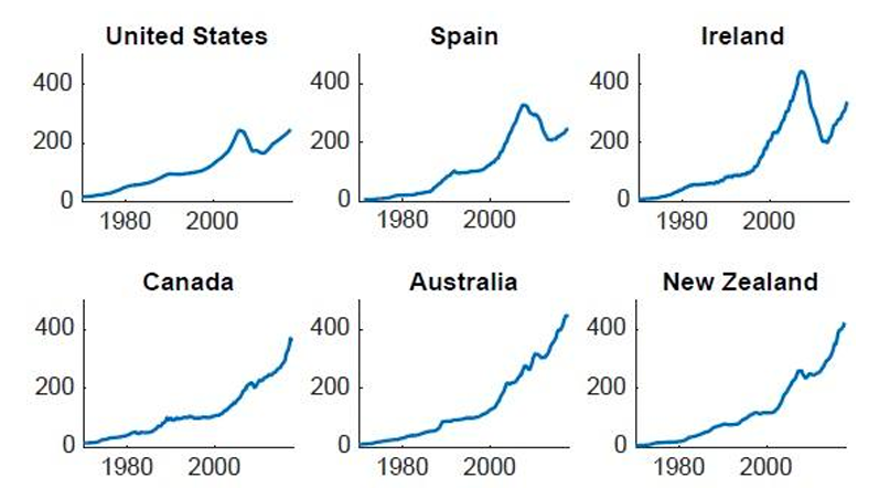
Source: IMF Global Housing Watch.

This section begins by gleaning lessons from across the globe, examining both the causes of housing booms and the timing of their eventual busts. In some cases, prior to a crisis, countries may have undergone a change or experienced an event that was unique and not broadly applicable. However, in many cases there are common threads that connect the experiences of different countries. From there, this section zooms in on the experience of the United States from the early 2000s to the financial crisis of 2008 and beyond. The availability of rich micro-level data and the presence of significant regional heterogeneity in economic conditions and legal environments has allowed researchers to put different theories to the test, whether using reduced-form empirical techniques or large structural models. Lastly, 9 this section discusses the latest research and avenues for future work on the macroeconomic consequences of housing crises.

As figure 2 illustrates, housing booms are not confined to any one country or time period, and neither are the busts that sometimes—but not always—follow. While it is appropriate to view each episode as resulting from a unique recipe of economic ingredients, there are also common themes undergirding many of the largest housing market swings observed over the past several decades. In an attempt to systematically approach the varying causes of booms and busts, it is useful to consider a modified version of the simple framework from the previous section. Consider a representative agent environment with utility , one-period mortgage debt , and a loan-to-value constraint that implies a minimum down payment ratio of . The first order conditions of the household’s optimization problem imply the following dynamic relationship for house prices:

where is rents, is the stochastic discount factor, now captures both depreciation and a discount that reflects the degree of illiquidity in the housing market, and is the Lagrange multiplier on the loan-to-value constraint. In a more general representative framework with the addition of a payment-to-income constraint and long-term debt, this expression takes on a similar form to that in Greenwald (2018):

Relative to the price equation in the simple framework, the main differences are the inclusion of timevarying illiquidity and the terms for the housing collateral premium, both of which subsequent sections discuss in detail. Importantly, this equation should be viewed as a conceptual device rather than an exact formula for house prices, given that it abstracts from other details pertaining to the legal and institutional environment as well as the degree of financial development. Specifically, to organize thinking for the remainder of this paper, let and stand in for the impact of credit, for the effect of “fundamentals” like income and demographics, for the importance of illiquidity, and for the role of expectations and beliefs.

Figure 2. Global Real House Prices

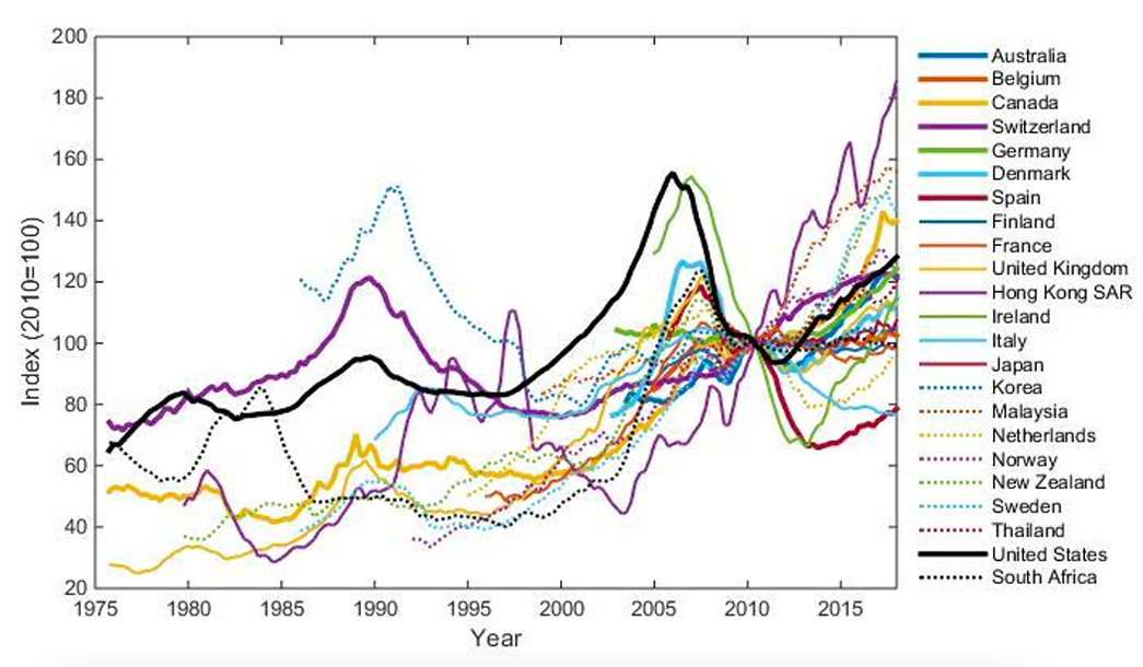
Source: Bank of International Settlements (BIS).

The Role of Fundamentals

Frequently, the term fundamentals is used to differentiate housing booms that can be explained by a rational model from those that require the addition of some other ad hoc ingredients or unstable “bubble” phenomena. Instead, for the purposes of this paper, fundamentals are factors that have an impact on house prices specifically through changes to rents—either implicit owner-equivalent rents or rents that can be observed directly. This distinction turns out to be important in light of the significant segmentation that exists in some countries between the owner-occupied and rental markets, which is studied in depth by Halket, Nesheim, and Oswald (2017).

Productivity

Although demand factors can play a significant role in driving short-run house prices with a total housing stock that is more or less fixed, construction costs are pivotal for explaining longer run movements. In the extreme case, constant returns to scale construction using labor and structures as inputs—with no fixed factor like land—implies that house prices exactly follow the path of relative productivity between the goods and construction sectors. Given that land accounted for only 10 percent of the value of houses from the beginning of the twentieth century through the years immediately following World War II, this assumption is not a bad approximation. In fact, Chambers, Garriga, and Schlagenhauf (2016) use an 11 equilibrium model with tenure choice between renting and owning to analyze the causes of the permanent increase in US house prices after World War II, concluding that the primary factor was indeed a relative slowdown in construction productivity growth that drove up costs. Similarly, Kahn (2008) generates large house price swings using a two-sector regime-switching model in which construction productivity grows at a constant rate but manufacturing productivity growth fluctuates over time. In that framework, manufacturing productivity booms produce house price booms. Kahn (2008) also estimates a low elasticity of substitution between housing and consumption and stresses its importance in generating large price swings, as seen in figure 3. Even so, while the model explains a significant fraction of the long-run increase in US house prices, it does not adequately replicate the large boom-bust episodes observed in the data.

Figure 3. (Left) US House Prices; (Right) Prices in a Regime Switch for Different Elasticities 

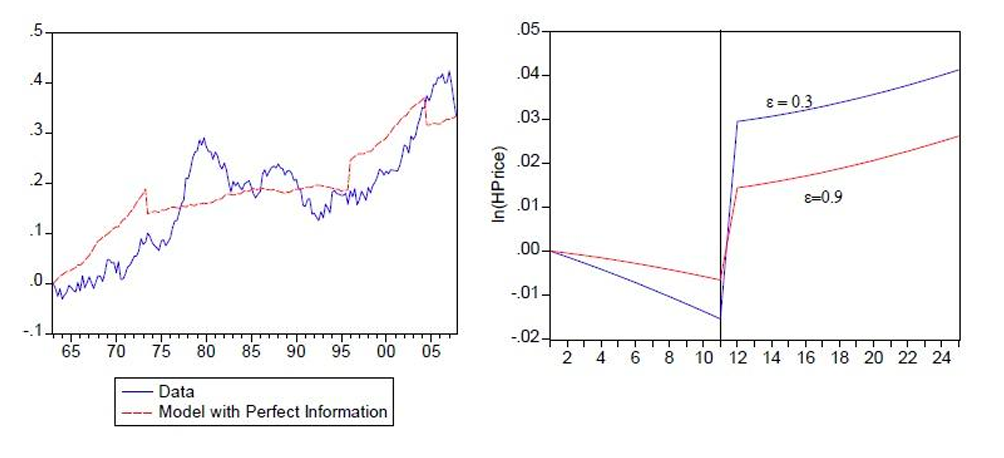Source: Figures 9 and 7, Kahn (2008).

Income and Wealth

Across countries and over time, there is a clear, positive relationship between housing costs and per-capita income. From the standpoint of theory, rents depend on the marginal rate of substitution between housing and consumption. Because the total stock of housing moves quite slowly, positive innovations to consumption—such as those driven by higher income—put upward pressure on rents and, therefore, house prices. For example, using a structural model with a fixed supply of houses, Sommer, Sullivan, and Verbrugge (2013) find that the increase in US real wages from 1995 to 2005 translated approximately 1:1 into higher prices and rents. Even over longer horizons, imperfectly elastic 12 construction arising from land supply constraints limits the extent to which the housing stock can expand to accommodate new demand.

Norway presents another compelling example of how rising income and wealth can drive up house prices. After the discovery of massive oil reserves in the North Sea, Norway’s crude oil production skyrocketed three-fold from 1980 to 1990 before doubling again by the year 2000. Around the same time, oil prices began an upward trajectory that culminated in a 300 percent increase from 2000 to 2009. During this twenty-year period from 1990 to 2010, Norway’s GDP growth greatly outpaced that of neighboring Sweden, and real house prices more than tripled.

These statistics do not imply that the entire Norwegian housing boom was driven by higher income, however. In fact, the IMF reports that Norway experienced one of the highest gains in the price-toincome ratio in Europe. Nevertheless, even if magnified by other factors such as cheap credit, fundamentals played an important role in the Norwegian experience over the past two decades. Unfortunately, going forward, the prospects for Norway’s housing market look less sanguine. With the fracking-induced drop in oil prices, Norway’s GDP growth has stalled, and its currency has depreciated by over 30 percent against the dollar since 2013. On top of these headwinds, Norway has recently implemented tighter mortgage controls and taken a more restrictive approach to immigration than neighboring Sweden. As a result, house price growth has turned negative over the past year, and policymakers are particularly concerned about the fragility of the housing market in the event that historically low mortgage rates start to rise. Many of these issues (e.g., migration, cheap credit, and macroeconomic fragility) are discussed in the remainder of this paper.

Demographics and Migration

Changes in an economy’s demographic structure, which can come from a multitude of sources, also generate significant adjustments in the housing market. In the United States, arguably one of the most notable examples was the post-World War II baby boom, which Mankiw and Weil (1989, p. 235) claim accounts for much of the growth in real house prices during the 1970s. Ironically, they also forecast that “if the historical relation between housing demand and housing prices continues into the future, real housing prices will fall substantially over the next two decades.” Of course, they could not have anticipated the profound shifts in the credit market that were about to begin unfolding, but that is a topic for future sections. One distinctive feature of demographic-driven housing booms—as contrasted by those fueled by cheaper credit—is their predictability, potential for sustainability, and the slow speed with which they unfold.

Migration—both internal and external—represents another dimension of demographic change that has important implications for the housing market. In the case of external migration, population flows of foreigners can generate sizable, albeit unpredictable, movements of house prices over short time horizons 13 in the face of relatively inelastic housing supply. Whether the migrants seek to own or rent is only of second-order importance, as both forces impact housing demand either directly or indirectly via the behavioral responses of investors. Returning to the comparison between Sweden and Norway, both countries experienced comparable rises in house prices between the early 1990s and 2010, even though Sweden lacked Norway’s oil reserves and GDP growth rate. However, Sweden made up for these shortcomings with higher immigration that, coupled with stringent rental market regulation, may have contributed to higher housing costs.

Although it may seem intuitive at first that higher immigration would drive up house prices, the literature does not speak with one voice on the matter. Some papers, such as Saiz (2007), find that immigration does indeed push up rents and house values in US destination cities. However, using UK data, Hatton and Tani (2005) as well as Sá (2014) both find that immigration has a negative effect on house prices. Whereas the positive studies seem to confirm the view that immigration contributes to higher total demand for housing, these latter two papers highlight how the evolving spatial distribution of the population affects house prices. Specifically, they find that areas experiencing a large influx of immigration witness an exodus of high-wage natives. Saiz and Wachter (2011) find corroborating evidence for this effect of residential sorting, while Guerrieri, Hartley, and Hurst (2013) show that its mirror image, gentrification, impacts house price dynamics through a positive externality whereby people want to live next to wealthy neighbors.

This form of residential sorting is absent, however, in cases where foreigners purchase houses but choose not to actually reside in them. In fact, this practice of out-of-town investors purchasing houses has become a significant trend in major urban centers such as Vancouver, Toronto, Sydney, and London— sometimes prompting significant public opposition because of the perception that it makes housing unaffordable. To analyze the impact of these out-of-town buyers, Favilukisand Van Nieuwerburgh (2018) develop and calibrate a heterogeneous agent spatial equilibrium model. They conclude that the observed increase in out-of-town purchases is responsible for 5 percent higher house prices in Vancouver but only 1.1 percent higher prices in New York.

Internal domestic migration can also produce housing booms in prices, quantities, or both. For example, Texas has experienced something of a population boom over the past two decades, though its vast availability of land and pro-development ethos have produced a larger boom in construction than in prices. By contrast, China has undergone a population shift of its own coupled with a surge in house prices. Not even four decades ago, nearly 80 percent of China’s population lived in rural areas. However, structural reforms and evolving global forces have prompted a shift in China’s economy toward urban manufacturing, and much of the population has relocated to where the jobs are. In recent research, Garriga, Hedlund, Tang, and Wang (2016) show that this large shift in the population to crowded urban areas can rationalize much of the rise in house prices.

Credit, Expectations, and the Housing Crisis Felt around the Globe

Each of the fundamental forces in the previous section has the ability to generate sustained booms or busts in house prices. However, the dramatic housing market swings in the United States and many other Western countries since 2000 have been characterized by large adjustments not just in house prices, but also in the price-rent ratio, indicating that other forces may also be at play. This section discusses what the latest research says about the ability of these other forces—namely, credit, liquidity, and expectations—to generate, amplify, and propagate large boom-bust episodes.

Figure 4. House Prices across States

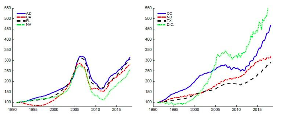
Source: Federal Housing Finance Agency (FHFA).

While it is tempting to discuss “the” post-2000 US housing boom and crisis—and indeed, its effects were experienced from coast to coast—significant heterogeneity can be seen in the dynamics of house prices within and across markets, as shown in figure 4. For example, the Sun Belt states faced a textbook housing cycle with a rapid appreciation of house prices in the early 2000s followed by a sudden and drastic collapse beginning in late 2006. For many of these states, an often-ignored issue is that the bust has been followed by a rapid recovery with prices now approaching their old peaks. However, in Washington, DC, and states like Colorado, Texas, and North Dakota, the Great Recession marked a mere pause in what is an ongoing housing boom. One cannot avoid noticing the similarities between the first set of volatile housing states and countries like Spain and Ireland as well as the second group of states and countries like Australia, Canada, and New Zealand, where house price appreciation continues unabated. Even though states operate within a relatively uniform national credit market and monetary policy, it is nevertheless unsurprising that the heterogeneous dynamics of prices across states mirror those observed between countries. After all, each state and country faces different economic conditions in terms of demographics, housing supply restrictions, and other factors that are partly responsible for the movements of house prices.

Expansions in Credit Supply: Empirical Evidence

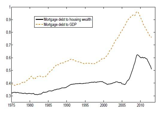
Green and Wachter (2007) report that nominal mortgage debt outstanding grew by 250 percent between 1997 and 2005. Relative to the size of the economy, this change represented an increase from just under 60 percent to almost 100 percent of GDP, as shown in figure 5. However, as a percentage of housing wealth, mortgage debt remained remarkably stable up until the collapse of house prices beginning in 2006. Thus, the key question is whether the growth in credit was one of the leading causes, or merely a symptom, of the housing boom and subsequent crisis.

Figure 5. Mortgage Debt 

Source: Figure 7, Davis and Van Nieuwerburgh (2015).

The asset pricing equation derived in the previous section specifies two margins of credit that impact house prices: access (i.e., constraints on quantities) and cost (i.e., interest rates). A large body of evidence points to a significant expansion of credit along both margins. First and easiest to measure is the decline in real mortgage rates from around 6 percent throughout the 1990s to only 4 percent beginning in the early 2000s. Much of this decline appears to be driven by changes in 10-year treasury rates. This was perhaps fueled by a global savings glut, as famously hypothesized by former Federal Reserve Chairman Bernanke, though Justiniano, Primiceri, and Tambalotti (2017) also identify a divergence beginning in 2003 when mortgage rates started lagging treasury yields.

There was also a significant aggregate expansion along the intensive and extensive margins of credit access during the boom, though a spirited debate continues regarding the distributional form that it took. In the early years of the crisis, the prevailing narrative attributed both the boom and the bust to excesses in the subprime market. As explained by Green and Wachter (2007), the traditional mortgage underwriting model focused on average cost pricing combined with rationing. If a prospective borrower was deemed 16 not credit worthy, the lender simply issued a loan denial. However, with the widespread adoption of credit scoring during the 1990s, lenders began tapping into a pool of marginal borrowers and offering credit at more expensive terms. In addition, lenders began offering more “exotic” mortgage products, such as loans that featured low initial “teaser” rates that most borrowers expected to refinance after accumulating some equity. Using rich micro-level data, Mian and Sufi (2009, 2011) were at the center of popularizing the argument that these innovations in credit access to risky borrowers fueled the boom and sowed the seeds for the crisis.

More recent research has begun to challenge the empirical foundations of this narrative. For example, Albanesi, De Giorgi, and Nosal (2017), using administrative credit panel data, provide a new narrative by showing that credit growth between 2001 and 2007 was actually concentrated in the prime market. Foote, Lowenstein, and Willen (2016) also claim that no such reallocation of credit occurred to risky borrowers, and in fact, wealthy borrowers actually accounted for most new debt in dollar terms. Digging deeper, Foote, Loewenstein, Nosal, and Willen (2018) point to housing investors—whom they define in the data as anybody with three or more first mortgages—as a key driver of the foreclosure crisis. Although these borrowers often had high income and credit scores, they were also more likely to transition from delinquency to foreclosure once prices started falling rather than attempt to cure their loans. At the same time, Lambie-Hanson et al (2019) show that investors have also contributed to the house price recovery. Anenberg et al. (2017) construct a measure of mortgage credit availability that traces out the maximum amount of debt obtainable by borrowers of different characteristics. Using data from 2001 to 2014, they find that the loan frontier expanded for all borrowers during the boom but contracted primarily for borrowers with low credit scores during the bust.

Mian and Sufi (2017) push back against this new narrative and claim that the growth in household debt from 2000 to 2007 was larger for individuals at the bottom of the credit score distribution, just as Bhutta and Keys (2016) find evidence in support of collateral constraints that bind especially for homeowners with low to middle credit scores. Progress with improved data quality and empirical methods will undoubtedly continue to inform this debate as time goes on. In fact, recent work by Greenwald (2018) and Cox and Ludvigson (2018) suggests that these dueling narratives are not mutually exclusive in light of evidence that most buyers prefer to take out the largest mortgage that they can qualify for. In other words, outside of all-cash transactions, most buyers are impacted by credit constraints.

The Interaction of Loose Credit Constraints and Low Mortgage Rates

A body of structural work has emerged in parallel to assess the contribution of lower mortgage rates and looser credit constraints to the boom, bust, and recovery in house prices. In one respect, economists have long recognized the potential of credit constraints to amplify fluctuations in house prices, as seen in classic 17 papers by Stein (1995) and Ortalo-Magné and Rady (2006). Yet, these earlier papers were a bit stylized and harder to take to the data. More recently, Favilukis, Ludvigson, and Van Nieuwerburgh (2017) claim that a relaxation of borrowing constraints and a decline in the housing risk premium—not lower interest rates—explain the boom in house prices. Garriga, Manuelli, and Peralta-Alva (forthcoming) also show that a decline in rates is not sufficiently potent by itself, but it can explain the boom when interacted with looser borrowing constraints. Justiniano, Primiceri, and Tambalotti (forthcoming) make a similar point for an isolated loosening of borrowing constraints, claiming that it would produce a counterfactual rise in mortgage rates due to higher borrowing in a closed economy model. Furthermore, Kaplan, Mitman, and Violante (2017) demonstrate that, in a model with perfectly integrated rental and owner-occupied markets, a loosening of down payment constraints cannot by itself reproduce the post-2000 boom in US house prices. Thus, it appears that, for the credit story to work, some combination of lower mortgage rates and looser borrowing constraints must be operative.

Illiquidity, Long-Term Debt, and Mortgage Default

Most of the previously discussed structural models abstract from one of the central topics investigated by the empirical literature: foreclosures and the response of credit supply to the risk of borrower default. Depending on market structure, incorporating mortgage default into macro-housing endogenizes the supply of credit to individual borrowers—either through risk-based pricing or rationing. However, going down this route entails significant computational costs. In a partial equilibrium setting with exogenous house prices, Corbae and Quintin (2015) use a framework with a rich menu of contract types to quantify the contribution of looser loan-to-value and payment-to-income constraints to the foreclosure crisis. They attribute over 60 percent of the rise in foreclosures to the increased prevalence of these loans in the later years of the boom.

The singular defining feature of housing crises is, above all, a large drop in house prices. In Corbae and Quintin (2015), this drop is manufactured exogenously, but other quantitative work studies the extent to which disruptions in credit can replicate the 25–30 percent US national decline in house prices (depending on the measure) between 2006 and 2011. In one paper, Chatterjee and Eyigungor (2015) reverse engineer a financial disruption that, in conjunction with an unexpected supply shock that increases the stock of houses, produces a 19 percent drop in prices. Garriga and Hedlund (2017) take a different approach by feeding in a combination of credit, labor market, and productivity shocks observed or inferred from the data. They are able to generate a 24 percent decline in house prices, and several lessons emerge regarding the driving forces behind this decline. First, higher downside risk in the labor market has the biggest single depressing effect on house prices, followed by a tightening in down payment constraints. Second, the model is highly nonlinear: the joint effect of the shocks exceeds the sum of the individual effects. Third, the endogenous response of housing illiquidity acts as a source of amplification and propagation.

This point about illiquidity merits extra discussion. In part prompted by the work of Kaplan and Violante (2014), there has been increasing realization over the past few years that the presence of illiquid assets on a household’s portfolio—most notably, housing—significantly affects behavior. Currently, the most common way in the literature of modeling illiquidity in the housing market is through the introduction of transaction costs reflected in the term in the house price equation from earlier. However, Garriga and Hedlund (2017) point out that the ease of buying and selling varies tremendously with housing conditions. At the peak of the 2000s boom, houses might sell within days or even instigate bidding wars, which stands in stark contrast to the trough, when houses might sit on the market for a year. Garriga and Hedlund (2017) go on to show that a deterioration in housing liquidity raises default risk, which in turn causes banks to cut credit. What emerges are liquidity spirals akin to those in Brunnermeier and Pedersen (2009) that amplify the house price decline during the bust by almost 27 percent.

In other work, Garriga and Hedlund (2018) point out that modeling mortgages accurately as long term debt is also crucial for explaining the dynamics of foreclosures and homeownership. Though useful for conceptual illustration, the loan-to-value constraint from earlier in this section, , has stark and counterfactual implications for crisis episodes. In words, this constraint states that the entirety of a borrower’s outstanding debt must satisfy a collateral constraint each period. Thus, a borrower’s ability to “pay off” their outstanding debt by taking out a new loan depends on the value of their housing collateral not falling too far. In the event that borrowers cannot roll their debt over into a new loan, they would be forced to either come up with cash or sell. In reality, collateral constraints are only imposed upon origination of a new mortgage and are therefore more aptly called down payment constraints. When house prices fall, nothing happens to homeowners who are able to continue making their scheduled amortization payments.

Credit and Market Segmentation

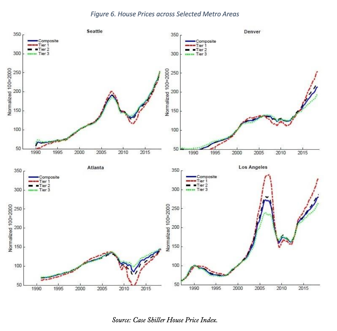
In the vast majority of quantitative structural models, housing enters the budget constraint as a quantity multiplied by a per-unit price, just like capital. The top row of figure 6 is largely consistent with this approach. In both Seattle and Denver, house prices across different market tiers followed roughly similar trajectories during the 2000s boom and crisis. However, the bottom row reveals two examples of divergent house price dynamics across market tiers. In Atlanta, prices in every segment of the housing market appeared to rise at similar rates during the housing boom, but the floor really fell out at the bottom end of the housing market during the bust. Los Angeles represents an even starker case of divergence that emerged during both the boom and the crisis.

Ríos-Rull and Sánchez-Marcos (2012) represent one of the earlier attempts at integrating fluctuating relative house prices into a quantitative model by replacing with in the household budget constraint and solving for equilibrium prices instead of just 1. More recently, Landvoigt, Piazzesi, and 20 Schneider (2015) have pioneered the use of rich micro-level data and an assignment model to explain price dynamics throughout San Diego. They conclude that cheaper credit for poor households was a major driver of prices in the lower tier of the market.

Preference Shocks, Beliefs, and Expectations

An alternative approach to producing shifts in housing demand relies on preference shocks. In one canonical paper, Iacoviello (2005) develops and estimates a two-agent model with preference shocks to housing; but while the model is able to match many cyclical features of the data, it cannot produce large housing booms and relies on one-period nominal debt to produce excessively strong collateral effects. In their absence, the preference shocks used to generate higher house prices actually produce a counterfactual, negative co-movement with consumption. Nevertheless, the paper does successfully establish the importance of including housing and nominal mortgage debt in business cycle models.

In the context of an incomplete-markets, heterogeneous-agent model, Kaplan, Mitman, and Violante (2017) also find that preference shocks generate a negative co-movement between house prices and consumption. Instead, they attribute the house price boom primarily to a belief shock about a future, yet ultimately unrealized, shift toward higher preferences for housing. While this framework can produce large swings in house prices, the nature of non-materializing preference shocks makes them completely unpredictable.

Broadly speaking, expectations undoubtedly play a critical role for house price behavior. For example, Case and Shiller (2003) find that homebuyers in the year 2003 thought that house prices would appreciate by an astonishing annual 9 percent over the next decade. According to them, this irrational enthusiasm in expectations concerning future prices was a major factor fueling the housing boom. Consistent with this view, Barlevy and Fisher (2010) argue that the prevalence of interest-only mortgages originated during the boom is evidence of a speculative bubble. Adam, Kuang, and Marcet (2012), Glaeser and Nathanson (2015), and Davis and Quintin (2017) develop models with sluggish expectations. In the case of the first two papers, this feature can produce house price behavior that is delinked from fundamentals, while Davis and Quintin (2017) emphasize the implications for default behavior. Along similar lines, Landvoigt (2017) finds that, contrary to the claims of Case and Shiller (2003), expectations of mean price growth were close to the long-run average during the boom. However, large subjective uncertainty about house price growth, given the option value of default, helps to explain the tremendous rise in household debt. Burnside, Eichenbaum, and Rebelo (2016) develop a stylized model of heterogeneous expectations and social contagion that generates booms that may or may not be followed by a bust. Lastly, Garriga, Manuelli, and Peralta-Alva (forthcoming) show that, even with perfectly rational agents, the slow arrival of information can drastically magnify the size of boom-bust episodes. Importantly, while many papers emphasize the role of beliefs in fueling the housing boom, they have a harder time explaining the bust in light of evidence provided by Cheng, Raina, and Xiong (2014) that the 21 agents who were most likely to be informed about real-time housing market conditions—managers in securitized finance—neither timed the market nor were cautious in their own home transactions, suggesting that they were unaware of an impending bust. Gerardi et al. (2008) offer further support for the unanticipated nature of the large price decline.

The Macroeconomic Consequences of Housing Crises

Clear evidence linking the US housing bust to the severity of the Great Recession is, by all accounts, largely responsible for reinvigorating interest among macroeconomists in the study of housing crises. A growing body of literature finds that large house price declines induce significant cuts to consumption as well as negative labor market spillovers, and can stunt the recovery after a recession. This section discusses the latest evidence and analysis of these macroeconomic effects.

Consumption and Balance Sheet Effects

Numerous papers and even an entire book by Gjerstad and Smith (2014) have highlighted the role of household balance sheets in transmitting housing market disruptions to consumption and employment. One prominent example is Mian and Sufi (2011), who use credit bureau data to identify a home equitybased borrowing channel whereby both new and existing homeowners extract equity from their houses when prices rise. Importantly, they find that households used this equity during the boom to increase consumption rather than pay down other high-interest debts or purchase investment properties, though Zhou (2018) has recently pushed back with evidence indicating that a large share of the borrowed funds were used for housing investment. Bhutta and Keys (2016) confirm the view that these borrowed funds were used either for consumption or illiquid investment rather than debt repayment based on the fact that equity extraction was associated with higher subsequent default risk, with Cooper (2013) providing further evidence against significant balance sheet repairs efforts by households.

A similar mechanism operates in reverse during housing busts. Empirically, Mian and Sufi (2014) show that employment contracted more strongly from 2007 to 2009 in counties that were more exposed to declines in house prices, and Mian, Rao, and Sufi (2013) find a similar negative effect on consumption at the zip code level. Garriga and Hedlund (2017) show that, in order to match the empirical facts, structural models should not abstract from portfolio composition. In particular, net worth is not a sufficient statistic for the response of consumption to changes in wealth—gross portfolio positions matter. Heavily indebted homeowners with more of their wealth in the form of housing experience larger declines in consumption than households with similar net worth but who are less exposed to the housing market. Garriga and Hedlund (2018) go further and point out the asymmetric response of consumption to house price changes in booms and busts, which they attribute in part to long-term debt and the option values of defaulting and refinancing.

Output and Production Linkages

Many of the previous papers have emphasized the transmission from housing to the macroeconomy through consumer spending, either as the main variable of interest or as a stand-in for “aggregate demand” that drives other components of GDP. However, there is growing evidence that housing crises also exert a macroeconomic impact by disrupting production chains and altering labor market flows. For example, Boldrin et al. (2016) address the ability of production linkages to induce a rippling effect through the rest of the economy from a decline in residential investment. They estimate that, although the drop in construction employment during the crisis only accounted directly for a modest fraction of the decline in total employment, a “production multiplier” arising from the input-output structure of the economy greatly magnified the impact. Quantitatively, they conclude that a $1 decline in demand in the construction sector generates a $2.10 decline in gross output, which, in the context of the Great Recession, means that the drop in housing output was responsible for up to 44 percent of the decline in total employment and 56 percent of the decline in output. The consequences of the construction collapse are particularly evident in states that experienced larger price declines, as seen in figure 7 below.

Figure 6. House Prices across Selected Metro Areas 

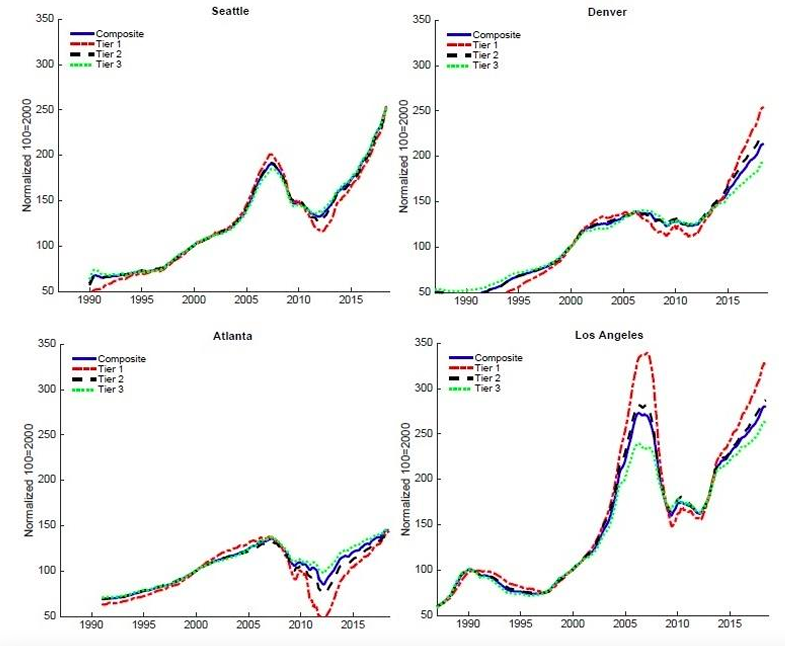
Source: Case Shiller House Price Index.

Labor Markets and Mobility

Turning attention to the labor market, Sterk (2015) presents both theoretical and empirical support for the idea that the evaporation of home equity during a crisis induces workers to turn down job offers that require them to move, either because of an inability to sell their previous house or afford a down payment in the new location. The empirical evidence is mixed, however, with Demyanyk, Hryshko, Luengo- 23 Prado, and Sorensen (2017) providing a contrary view. They interpret empirical evidence from merged individual-level credit reports and loan-level mortgage data through the lens of a structural model and conclude that negative equity during the crisis was not a significant barrier to mobility. However, Brown and Matsa (2016) do find evidence for a negative mobility response in areas with depressed housing markets, especially when the legal environment features recourse mortgages. Van Veldhuizen, Vogt, and Voogt (2018) use administrative panel data of nearly the entire population of Dutch homeowners to arrive at similar findings abroad. Together, these last two papers indicate that foreclosure laws may play a critical role in shaping the response of job search behavior to deteriorating housing market conditions.

Lessons from Emergency Policy Interventions

For policymakers, the practical question that inevitably comes to mind after understanding the causes and consequences of housing crises is, “What can we do about it?” The range of experiences across states and countries over the last decade has proven fruitful for researchers as they assess the impacts of policies that have already been implemented and contemplate possible future actions. This section focuses only on housing-related legislative interventions implemented during the Great Recession. Although important, this section does not discuss the response of monetary policy, the role of automatic stabilizers such as unemployment benefit extensions, or the ability of macroprudential policy to reduce the likelihood of future housing crises. Lessons from these interventions can, however, provide guideposts for how to reduce the severity of a future crisis if one is to emerge.

Direct Debt Relief

Congress intervened with the creation of the Home Affordable Modification Program (HAMP) and Home Affordable Refinance Program (HARP), which were targeted programs aimed at preventing distressed or underwater borrowers from going into foreclosure. The principal distinction was that HAMP modified the existing mortgage contract of a borrower (e.g., by extending the loan term, reducing the interest rate, or cutting the monthly payment), whereas HARP streamlined and loosened underwriting requirements for borrowers with negative equity to allow them to take out a new loan at prevailing market rates. California also instituted its own series of “Keep Your Home California” initiatives, including a principal reduction program.

A stream of recent papers has evaluated the consequences of these programs. On the empirical front, Agarwal et al. (2017) exploit regional variation in the intensity of HAMP implementation and find evidence that the program had a salutary effect on foreclosures, house prices, and durable spending. However, the program only reached one third of its intended audience of highly indebted households. One of the central policy questions surrounding these programs is whether principal reductions or interest rate relief are more potent forms of “stimulus.” The lesson that emerges from the structural analyses in Hedlund (forthcoming) and Kaplan, Mitman, and Violante (2017) is that principal reductions can 24 significantly reduce foreclosures but are not effective by themselves at boosting house prices or consumption. Recent work by Ganong and Noel (2018) provides empirical support for this finding. In particular, they use variation in mortgage modifications to separate the wealth effect from the cash-flow effect of debt reduction. Their empirical design reveals that principal reductions that leave liquidity unchanged (i.e., they do not relax budget constraints) have no effect on consumption. By contrast, interventions that provide liquidity relief without changing balance sheets, such as loan maturity extensions, have large effects.

Altering Foreclosure Laws

Several lessons emerge from a large body of work that emphasizes the importance of foreclosure laws. For example, Ghent and Kudlyak (2011) examine how the propensity to default is impacted by recourse laws (laws which allow banks to pursue deficiency judgments from borrowers for outstanding mortgage debt not paid off by the foreclosure sale). They find that recourse lowers borrowers’ sensitivity to negative equity, thereby mitigating the strategic motive to default, which Gerardi et al. (2018) claim plays a role in nearly 40 percent of mortgage defaults. However, Hatchondo, Martinez, and Sanchez (2015) point out that the relationship between recourse stringency and foreclosure activity is non-monotonic. With stricter foreclosure laws, borrowers undoubtedly have a lower individual propensity to default for a given level of debt, but banks respond by expanding the supply of credit, which may increase the amount of debt in the economy. Empirically, although Hurst et al. (2016) find substantial mortgage market redistribution across regions that could mute the impact of state-specific laws, Li and Oswald (2017) show that legislation passed in Nevada in 2009 that abolished deficiency judgments led to a contraction in credit. In terms of macroeconomic impact, Hedlund (2016) finds that recourse laws induce greater caution among buyers when purchasing and financing houses, which reduces the volatility of house prices.

Mian, Sufi, and Trebbi (2015) identify strong macroeconomic effects from another significant source of state-level variation in foreclosure laws: the presence or absence of a judicial requirement that requires lenders to seek court permission to initiate foreclosure proceedings. They provide evidence for a discrete jump in foreclosures upon crossing the border into a state without a judicial requirement, and this elevated foreclosure activity led to a large decline in house prices and consumption between 2007 and 2009. However, these states also subsequently experienced a faster rebound during the recovery, which lends credence to the analysis in Guren and McQuade (2018) that demonstrates how foreclosure delays may be counterproductive even in the presence of the damaging foreclosure externalities that both they as well as Anenberg and Kung (2014) find.

Herkenhoff and Ohanian (forthcoming) show how foreclosure delays act as an implicit line of credit that leads to longer unemployment spells by altering job search behavior. Using micro data, they show that these delays depressed employment during the Great Recession by up to 1.3 percentage points in states 25 like Florida and New Jersey, which seems to confirm the assertion by Guren and McQuade (2018) that foreclosure delays can be economically detrimental.

Stimulating Housing Sales

In addition to these measures targeted at distressed borrowers, the federal government instituted a $20 billion First-Time Homebuyer Credit (FTHC) between 2008 and 2010 to stimulate home buying and prices. At the time, one worry that emerged was that any beneficial effects would immediately reverse upon conclusion of the policy. After all, multiple studies have highlighted the ineffectiveness of the 2009 Cash for Clunkers program. Specifically, Mian and Sufi (2012) exploit variation in exposure to the Cash for Clunkers program across cities and find strong evidence that higher initial sales caused by the program initially were completely offset by lower future sales. Furthermore, Hoekstra, Puller, and West (2017) show that Cash for Clunkers actually reduced total new vehicle spending by $5 billion by inducing a shift to less expensive cars.

Berger, Turner, and Zwick (2018) analyze the FTHC program with these concerns in mind but arrive at far different conclusions. Using administrative tax records combined with transaction deeds data, they find that (1) the policy spurred sales and homeownership, (2) these effects did not reverse after the program ended, and (3) the main benefit of the policy was to accelerate the process of reallocation of existing houses from distressed sellers to high-value buyers rather than provide direct stimulus to new construction. Furthermore, these positive effects were likely not confined to the housing market. Adding to the abundant evidence described earlier in the paper on consumption and balance sheet effects, Benmelech, Guren, and Melzer (2018) show that home sales have a significant spillover impact on purchases of durable goods.

Summary of Emergency Intervention Policy Lessons

1. Interventions that provide cash-flow relief (e.g., policies that allow underwater borrowers to refinance when rates fall) are more effective at boosting house prices and consumption than are principal reductions that do little to alleviate strain on household budgets.
2. Attempts to either forcibly delay banks from instituting the foreclosure process on delinquent borrowers (e.g., judicial requirements) or to soften the consequences of default (e.g., abolishing deficiency judgments) often do more harm than good by inducing a contraction in the supply of credit and lengthening unemployment spells.
3. Unlike the highly ineffective Cash for Clunkers program, policies that stimulate home purchases create long-lasting increases in sales, house prices, and, in light of abundant evidence on spillovers, higher consumer spending as well.

Conclusions and Directions for Future Research

As the largest source of wealth for most people, housing has always played an outsized role in economic life. However, the pace of financial innovation, credit market liberalization, and globalization over the past few decades has increased the chance that local housing downturns turn into more severe crises that cause lasting macroeconomic damage. This article has provided a guided tour for the leading explanations behind the causes and consequences of housing crises with an attempt to blend reduced-form empirical evidence with structural analysis.

Going forward, there are many fruitful areas that demand further research. For example, economists still lack a satisfactory structural model that can quantitatively account for all of the stylized facts of house prices documented earlier in this article, with house price momentum proving the most challenging. In addition, while convenient for aggregate analysis, it is clear that treating housing as a unified national market is strongly counterfactual. Instead, the next generation of models should continue to incorporate insights from the micro-data to explain heterogeneous housing dynamics across regions, price tiers, buyer type (e.g., owner-occupier vs. investor), and market segment (e.g., new construction vs. existing housing). The issue of segmentation is also relevant with regard to the housing finance system and the relationship between the rental and owner-occupied market, both of which are critical to forecasting the risk of future housing crashes. For example, why have house prices rebounded since their trough in 2011 while construction has lagged behind, and to what extent can sluggish construction explain rapidly rising prices in places like Dallas, Texas, which witnessed only modest house price growth during the previous boom?

To better understand the anatomy of housing crises, more research is needed to understand the link between housing and other markets—especially the labor market. While the health of the labor market— both on the demand side through job creation and on the supply side through internal and external migration—undoubtedly affects the strength of housing, causality can run the other way as well. For example, there is ongoing uncertainty about the extent to which negative equity creates house lock that limits geographic mobility. On the one hand, negative equity makes it more difficult for homeowners to sell their house to move to opportunity. On the other hand, if the opportunity is sufficiently attractive, owners may be willing to default on their mortgage and leave anyway, depending on the severity of state level foreclosure consequences.

Beyond the labor market, housing is both strongly affected by and a primary driver of activity in capital markets. It can facilitate small business investment by serving as a form of collateral, but it can also compete for funds and time against other forms of investment. For policymakers, knowledge of these spillovers is of paramount importance, as is understanding how different institutional features of the housing finance system affect the dynamism and resiliency of housing markets. For example, do policies that subsidize homeownership promote economic opportunity and wealth creation, or do they sow instability by encouraging excess leverage? Furthermore, to what extent does the answer to this question 27 depend on institutional details such as mortgage contract design, the structure of the banking sector and its regulatory architecture, and the conduct of monetary and fiscal policy? These questions are in some sense just the tip of the iceberg, and answering them will require a new generation of structural models, empirical analysis, and granular micro-data to give a more complete picture of how to mitigate future crisis episodes.

References

Adam, Klaus, Pei Kuang, and Albert Marcet. 2012. “House Price Booms and the Current Account.”
NBER Macroeconomics Annual 26 (1): 77–122.
Agarwal, Sumit, Gene Amromin, Itzhak Ben-David, Souphala Chomsisengphet, Tomasz Piskorski, and Amit Seru. 2017. “Policy Intervention in Debt Renegotiation: Evidence from the Home Affordable Modification Program.” Journal of Political Economy 125 (3): 654–712.
Albanesi, Stefania, Giacomo De Giorgi, and Jaromir Nosal. 2017. “Credit Growth and the Financial Crisis: A New Narrative.” NBER Working Paper 23740. National Bureau of Economic Research, Cambridge, MA.
Anenberg, Elliot, and Edward Kung. 2014. “Estimates of the Size and Source of Price Declines Due to Nearby Foreclosures.” American Economic Review 104 (8): 2527–51.
Anenberg, Elliot, Aurel Hizmo, Edward Kung, and Raven Molloy. 2017. “Measuring Mortgage Credit Availability: A Frontier Estimation Approach.” FEDS Working Paper No. 2017-101.
Barlevy, Gadi, and Jonas D. M. Fisher. 2010. “Mortgage Choices and Housing Speculation.” FRB Chicago Working Paper.
Benmelech, Efraim, Adam Guren, and Brian T. Melzer. 2018. “Making the House a Home: The Stimulative Effective of Home Purchases on Consumption and Investment.” NBER Working Paper 23570. National Bureau of Economic Research, Cambridge, MA.
Berger, David, Nicholas Turner, and Eric Zwick. Forthcoming. “Stimulating Housing Markets.” Journal of Finance
Bhutta, Neil, and Benjamin J. Keys. 2016. “Interest Rates and Equity Extraction During the Housing Boom.” American Economic Review 106 (7): 1742–74.
Boldrin, Michele, Carlos Garriga, Adrian Peralta-Alva, and Juan Sanchez. 2016. “Reconstructing the Great Recession.” FRB St. Louis Working Paper No. 2013-006C.
Brown, Jennifer and David A. Matsa. 2016. “Locked in by Leverage: Job Search During the Housing Crisis.” Working Paper.
Brunnermeier, Markus K., and Lasse Heje Pedersen. 2009. “Market Liquidity and Funding Liquidity.”
Review of Financial Studies 22 (6): 2201–38.
Campbell, John, and Robert Shiller. 1988a. “Stock Prices, Earnings and Expected Dividends.” Journal of Finance 43 (3): 661–76.
———. 1988b. “The Dividend-Price Ratio and Expectations of Future Dividends and Discount Factors.” Review of Financial Studies 1 (3): 195–228.
Campbell, Sean D., Morris A. Davis, Joshua Gallin, and Robert F. Martin. 2009. “What Moves Housing Markets: A Variance Decomposition of the Rent-Price Ratio.” Journal of Urban Economics 66 (2): 90–102.
Case, Karl E., and Robert J. Shiller. 1989. “The Efficiency of the Market for Single-Family Homes.”
American Economic Review 79, no. 1 (March): 125–37.
———. 2003. “Is There a Bubble in the Housing Market?.” Brookings Papers on Economic Activity no. 2, 299–362.
Chambers, Matthew, Carlos Garriga, and Don Schlagenhauf. 2016. “The Postwar Conquest of the Home Ownership Dream.” FRB St. Louis Working Paper No. 2016-7.
Chatterjee, Satyajit, and Burcu Eyigungor. 2015. “A Quantitative Analysis of the U.S. Hous- ing and Mortgage Markets and the Foreclosure Crisis.” Review of Economic Dynamics 18 (2): 165–84.
Cheng, Ing-Haw, Sahil Raina, and Wei Xiong. 2014. “Wall Street and the Housing Bubble.”American Economic Review 104 (9): 2797–829.
Cooper, Daniel H. 2013. “Changes in U.S. Household Balance Sheet Behavior after the Housing Bust and Great Recession: Evidence from Panel Data.” FRB of Boston, Public Policy Discussion Paper No. 13-6.
Corbae, Dean, and Erwan Quintin. 2015. “Leverage and the Foreclosure Crisis.” Journal of Political Economy 123:1–65.
Cox, Josue, and Sydney C. Ludvigson. 2018. “Drivers of the Great Housing Boom-Bust: Credit Conditions, Beliefs, or Both?.” NBER Working Paper No. 25285. National Bureau of Economic Research, Cambridge, MA.
Davis, Morris A., and Erwan Quintin. 2017. “On the Nature of Self-Assessed House Prices.” Real Estate Economics 45 (3): 628–49.
Davis, Morris A., and Jonathan Heathcote. 2005. “Housing and the Business Cycle.” International Economic Review 46 (3): 751–84.
———. 2007. “The Price and Quantity of Residential Land in the United States.” Journal of Monetary Economics 54:2595–620.
Davis, Morris A., Andreas Lehnert, and Robert F. Martin. 2008. “The Rent-Price Ratio for the Aggregate Stock of Owner-Occupied Housing.” Review of Income and Wealth 54 (2): 279–84.
Davis, Morris, and Stijn Van Nieuwerburgh. 2015. “Housing, Finance and the Macroeconomy.”
Handbook of Regional and Urban Economics 5:753–811.
Demyanyk, Yuliya, Dmytro Hryshko, María Jose Luengo-Prado, and Bent E. Sorensen. 2017. “Moving to a Job: The Role of Home Equity, Debt, and Access to Credit.” American Economic Journal: Macroeconomics 9 (2): 149–181.
Favilukis, Jack, and Stijn Van Nieuwerburgh. 2018. “Out-of-Town Home Buyers and City Welfare.,” Working Paper
Favilukis, Jack, Sydney C. Ludvigson, and Stijn Van Nieuwerburgh. 2017. “The Macroeconomic Effects of Housing Wealth, Housing Finance, and Limited Risk-Sharing in General Equilibrium.” Journal of Political Economy 125 (1): 140–223.
Foote, Christopher L., Lara Lowenstein, and Paul S. Willen. 2016. “Cross-Sectional Patterns of Mortgage Debt during the Housing Boom: Evidence and Implications.” NBER Working Paper No. 22985. National Bureau of Economic Research, Cambridge, MA.
Foote, Christopher, Lara Loewenstein, Jaromir Nosal, and Paul Willen. 2018. “Maybe Some People Shouldn’t Own (3) Homes.” 2018 Meeting Papers 922. Society for Economic Dynamics.
Ganong, Peter, and Pascal Noel. 2018. “Liquidity vs. Wealth in Household Debt Obligations: Evidence from Housing Policy in the Great Recession.” NBER Working Paper No. 24964. National Bureau of Economic Research, Cambridge, MA.
Garriga, Carlos, Aaron Hedlund, Yang Tang, and Ping Wang. 2017. “Rural-Urban Migration, Structural Transformation, and Housing Markets in China.” NBER Working Paper No. 23819. National Bureau of Economic Research, Cambridge, MA.
Garriga, Carlos, and Aaron Hedlund. 2017. “Mortgage Debt, Consumption, and Illiquid Housing Markets in the Great Recession.” FRB St. Louis Working Paper No. 2017-30.
———. 2018. “Housing Finance, Boom-Bust Episodes, and Macroeconomic Fragility.” 2018 Meeting Papers 354. Society for Economic Dynamics.
Garriga, Carlos, Rody Manuelli, and Adrian Peralta-Alva. Forthcoming. “A Macroeconomic Model of Price Swings in the Housing Market.” American Economic Review.
Gerardi, Kris, Kyle Herkenhoff, Lee E. Ohanian, and Paul Willen. 2018. “Can’t Pay or Won’t Pay? Unemployment, Negative Equity, and Strategic Default.” Review of Financial Studies 31 (3): 1098–131.
Gerardi, Kristopher, Andreas Lehnert, Shane M. Sherlund, and Paul Willen. 2008. “Making Sense of the Subprime Crisis.” Brookings Papers on Economic Activity 36, no. 2 (Fall): 69–159.
Ghent, Andra, and Marianna Kudlyak. 2011. “Recourse and Residential Mortgage Default: Evidence from U.S. States.” Review of Financial Studies 24 (9): 3139–86.
Gjerstad, Steven D., and Vernon L. Smith. 2014. Rethinking Housing Bubbles: The Role of Household and Bank Balance Sheets in Modeling Economic Cycles. Cambridge UK: Cambridge University Press.
Glaeser, Edward L., and Charles G. Nathanson. 2015. “Housing Bubbles.” Handbook of Regional and Urban Economics 5:701–51.
Green, Richard, and Susan M. Wachter. 2007. “The Housing Finance Revolution.” Proceedings, Federal Reserve Bank of Kansas City.
Greenwald, Daniel. 2018. “The Mortgage Channel of Macroeconomic Transmission.” Working Paper.
Guerrieri, Veronica, Daniel Hartley, and Erik Hurst. 2013. “Endogenous Gentrification and Housing Price Dynamics.” Journal of Public Economics 100:45–60.
Guren, Adam, and Tim McQuade. 2018. “How do Foreclosures Exacerbate Housing Downturns?.” Boston University Department of Economics Working Paper No. WP2018-007.
Halket, Jonathan, Lars Nesheim, and Florian Oswald. 2017. “The Housing Stock, Housing Prices, and User Costs: The Roles of Location, Structure and Unobserved Quality.” Cemmap Working Paper CWP73/15. Center for Microdata Methods and Practice, Institute of Fiscal Studies, London, UK.
Hatchondo, Juan Carlos, Leonardo Martinez, and Juan M. Sanchez. 2015. “Mortgage Defaults.” Journal of Monetary Economics 76:173–90.
Hatton, Timothy J., and Massimiliano Tani. 2005. “Immigration and Interregional Mobility in the UK, 1982–2000.” Economic Journal 115:F342–58.
Head, Allen, Huw Lloyd-Ellis, and Hongfei Sun. 2014. “Search, Liquidity, and the Dynamics of House Prices and Construction.” American Economic Review 104 (4): 1172–210.
Hedlund, Aaron. 2016. “The Cyclical Dynamics of Illiquid Housing, Debt, and Foreclosures.”
Quantitative Economics 7 (1): 289–328.
———. Forthcoming. “Failure to Launch: Housing, Debt Overhang, and the Inflation Option.”
American Economic Journal: Macroeconomics.
Herkenhoff, Kyle, and Lee Ohanian. Forthcoming. “The Impact of Foreclosure Delay on U.S. Employment.” Review of Economic Dynamics.
Hoekstra, Mark, Steven L. Puller, and Jeremy West. 2017. “Cash for Corollas: When Stimulus Reduces Spending.” American Economic Journal: Applied Economics 9 (3): 1–35.
Hurst, Erik, Benjamin J. Keys, Amit Seru, and Joseph Vavra. 2016. “Regional Redistribution through the US Mortgage Market.” American Economic Review 106 (10): 2982–3028.
Iacoviello, Matteo. 2005. “House Prices, Borrowing Constraints, and Monetary Policy in the Business Cycle.” American Economic Review 95 (3): 739–64.
Jeske, Karsten, Dirk Krueger, and Kurt Mitman. 2013. “Housing, Mortgage Bailout Guarantees and the Macro Economy.” Journal of Monetary Economics 60 (8): 917–35.
Jordà, Òscar, Moritz Schularick, and Alan Taylor. 2015a. “Betting the House.” Journal of International Economics 96:S2–S18.
Justiniano, Alejandro, Giorgio E. Primiceri, and Andrea Tambalotti. 2017. “The Mortgage Rate Conundrum.” FRB of Chicago Working Paper No. WP-2017-23.
———. Forthcoming. “Credit Supply and the Housing Boom.” Journal of Political Economy. Kahn, James A. 2008. “What Drives Housing Prices?.” FRB of New York, Staff Report No. 345. Kaplan, Greg, and Giovanni L. Violante. 2014. “A Model of the Consumption Response to Fiscal
Stimulus Payments.” Econometrica 82 (4): 1199–239.
Kaplan, Greg, Kurt Mitman, and Giovanni L. Violante. 2017. “The Housing Boom and Bust: Model Meets Evidence.” NBER Working Paper No. 23694. National Bureau of Economic Research.
Kindleberger, Charles P. 1993. A Financial History of Western Europe. Oxford, UK: Oxford University Press.
Kiyotaki, Nobuhiro, Alexander Michaelides, and Kalin Nikolov. 2011. “Winners and Losers in Housing Markets.” Journal of Money, Credit, and Banking 43, no. 2–3 (March): 255–96.
Lambie-Hanson, Lauren, Wenli Li, and Michael Slonkosky. 2019. “Leaving Households Behind: Institutional Investors and the U.S. Housing Recovery” FRB Philadelphia Working Paper No. 19-01.
Landvoigt, Tim. 2017. “Housing Demand During the Boom: The Role of Expectations and Credit Constraints.” Review of Financial Studies 30 (6): 1865–902.
Landvoigt, Tim, Monika Piazzesi, and Martin Schneider. 2015. “The Housing Market(s) of San Diego.”
American Economic Review 105 (4): 1371–407.
Leamer, Edward E. 2007. “Housing is the Business Cycle.” Proceedings, Federal Reserve Bank of Kansas City, 149–233.
Li, Wenli, and Florian Oswald. 2017. “Recourse and Residential Mortgages: The Case of Nevada.”
Journal of Urban Economics 101:1–13.
Mankiw, N. Gregory, and David N. Weil. 1989. “The Baby Boom, the Baby Bust, and the Housing Market.” Regional Science and Urban Economics 19:235–58.
Mian, Atif, Amir Sufi, and Francesco Trebbi. 2015. “Foreclosures, House Prices, and the Real Economy.” Journal of Finance 70 (6): 2587–634.
Mian, Atif, and Amir Sufi. 2009. “The Consequences of Mortgage Credit Expansion: Evidence from the
U.S. Mortgage Default Crisis.” Quarterly Journal of Economics 124, no. 4 (November): 1449–96.
———. 2011. “House Prices, Home Equity-Based Borrowing, and the US Household Leverage Crisis.”
American Economic Review 101 (5): 2132–56.
———. 2012. “The Effects of Fiscal Stimulus Evidence from the 2009 Cash for Clunkers Program.”
Quarterly Journal of Economics 127 (3): 1107–42.
———. 2014. “What Explains the 2007–2009 Drop in Employment?.” Econometrica 82 (6): 2197–223.
———. 2017. “Household Debt and Defaults from 2000 to 2010: The Credit Supply View.” In Innovation in Housing Law and Policy, edited by Lee Anne Fennell and Benjamin J. Keys. Cambridge, UK: Cambridge University Press.
Mian, Atif, Kamalesh Rao, and Amir Sufi. 2013. “Household Balance Sheets, Consumption, and the Economic Slump.” Quarterly Journal of Economics 128 (4): 1687–726.
Ortalo-Magn´e, Fran¸cois, and Sven Rady. 2006. “Housing Market Dynamics: On the Contribution of Income Shocks and Credit Constraints.” Review of Economic Studies 73, no. 2 (April): 459–85.
Piazzesi, Monika, and Martin Schneider. 2016. “Housing and Macroeconomics.” In Handbook of Macroeconomics Volume 2a, edited by John B. Taylor and Harald Uhlig, 1547–640. Amsterdam: Elsevier.
Piazzesi, Monika, Martin Schneider, and Selale Tuzel. 2007. “Housing, Consumption and Asset Pricing.” Journal of Financial Economics 83:531–69.
S´a, Filipa. 2014. “Immigration and House Prices in the UK.” Economic Journal 125:1393–424.
Saiz, Albert. 2007. “Immigration and Housing rents in American Cities.” Journal of Urban Economics 61 (2): 345–71.
Saiz, Albert, and Susan Wachter. 2011. “Immigration and the Neighborhood.” American Economic Journal: Economic Policy 3:169–88.
Sommer, Kamila, and Paul Sullivan. 2018. “Implications of US Tax Policy for House Prices, Rents, and Homeownership.” American Economic Review 108 (2): 241–74.
Sommer, Kamila, Paul Sullivan, and Randal Verbrugge. 2013. “The Equilibrium Effect of Fundamentals on House Prices and Rents.” Journal of Monetary Economics 60 (7): 854–70.
Stein, Jeremy C. 1995. “Prices and Trading Volume in the Housing Market: A Model with Down- Payment Effects.” Quarterly Journal of Economics 110, no. 2 (May): 379–406.
Sterk, Vincent. 2015. “Home Equity, Mobility, and Macroeconomic Fluctuations.” Journal of Monetary Economics 74:16–32.
Van Veldhuizen, Sander, Benedikt Vogt, and Bart Voogt. Forthcoming. “Negative Home Equity Reduces Household Mobility: Evidence from Administrative Data.” Journal of Housing Economics.
Zhou, Xiaoqing. 2018. “Home Equity Extraction and the Boom-Bust Cycle in Consumption and Residential Investment.” 2018 Meeting Papers 795. Society for Economic Dynamics.