Strategic Reporting and the Effects of Water Use in Hydraulic Fracturing on Local Groundwater Levels in Texas

Backstrom, Jesse

Introduction

High-volume hydraulic fracturing, conducted after the drilling of a wellbore, is the primary completion technique used to stimulate the flow of hydrocarbons from low-permeability, unconventional reservoirs. Its use has increased rapidly in the U.S. over the last decade and a half, and a common complaint among communities located near unconventional oil and gas production is that they felt unprepared to handle the rapid pace of its development, especially the water use of the industry (Freyman 2014; Gold 2014). Over time, an increasingly large volume of water has been used to stimulate each well, heightening concerns over the potential impacts on local availability.¹ According to U.S. EPA (2016), the impacts on groundwater can be large, although they are dependent on the balance between withdrawals and the resource stock and recharge rate at a given point.

In my dataset, median water use for a horizontal well was almost 11.2 million gallons in Texas in early 2017, which is up from about 3.8 million in 2012. In the Permian Basin in west Texas, where the largest share of unconventional oil is now being produced,² median water use per well was over 14.6 million gallons in early 2017—the equivalent to supplying about 91,000 average two-person U.S. households with water for a day, or 250 households with water for a year.³ Although they are helpful in characterizing the water use of the industry, previous studies in the economics and natural sciences literatures have only descriptively analyzed the industry’s historical water use and its future needs, and discussed potential externalities affecting local water quality and availability.

In this paper, I am the first to empirically investigate two interrelated issues concerning the industry’s water use. First, using a unique dataset of completion reports for hydraulically stimulated wells in Texas,⁴ I analyze the influence of local groundwater management regimes on the level of detail that upstream oil and gas producers (operators hereafter) use when reporting their water use. I test the hypothesis that completion reports submitted for wells located in a groundwater conservation district (GCD) are less detailed, i.e., contain the bare minimum information on water use that is required, relative to those for wells not in a GCD. Since operators prefer freshwater due to little or no costly purification or treatments needed to make it usable, I argue they also have preferences for a continued ability to use freshwater.⁵,⁶,⁷ Given plausible operator knowledge on the effects of their water use, concerns over water availability in Texas, and expectations over future regulations that may increase the costs to access and or acquire water, it is clear they have an incentive to leave less of a paper trail when reporting water use, particularly in water-scarce areas (hence, the need for GCDs).

Second, I use a high-frequency dataset from the Texas Water Development Board (TWDB) to test the hypothesis that the amount of water used in hydraulic fracturing is large enough to have an empirically discernable effect on groundwater levels near unconventional oil and gas development. Since surface waters are owned by the state of Texas and surface water rights are allocated, this issue is made more salient by the fact that lucrative markets have developed throughout the state where landowners sell their water rights and or pump groundwater in relatively unrestricted quantities and sell it to operators or other midstream water distribution firms.⁸ Larger effects of the industry’s water use are expected in the more arid regions, such as those where the Permian and Eagle Ford Basins are located, where most of the hydraulic fracturing activity is occurring and groundwater is the primary source of water for drilling and completion activities.⁹

I find that operators of wells located in a GCD area are more likely by 1.3–2.8 percentage points to omit key details of their water use. I also find a similar relationship with respect to actual water use, as the propensity to report more than a minimum amount of detail decreases with larger amounts of water used to stimulate a well, and for horizontally and directionally drilled wells relative to their vertically drilled counterparts. These findings are consistent with the idea that operators respond to disclosure requirements in strategic ways, particularly if they forestall other regulations that are expected to be costlier (Lyon and Maxwell 2004; 2008). In the model of groundwater levels, I show a causal link between the volume of water used in hydraulic fracturing and declining groundwater availability. I estimate that a 73-million-gallon increase (roughly five new 2017 Permian Basin wells) in the monthly amount of water used in hydraulic fracturing within a 10-mile radius of a groundwater monitoring station leads to a drop in the groundwater level by 1.93 feet. I also find heterogeneous impacts for cumulative water use in GCD vs. non-GCD areas, and in the Permian and Eagle Ford regions relative to other areas in the state. The findings in this paper provide the first credible evidence that water use in hydraulic fracturing affects local water availability, and they emphasize the importance of transparency in reporting for water management.

Literature Review

A growing literature in economics has studied many of the positive and negative local economic impacts of the “shale boom.” The general consensus is that the economic benefits are large, but further research is needed to understand the magnitude and extent of the negative effects (Mason et al. 2015). Bartik et al. (2017) study the local welfare consequences and estimate a willingness to pay to prevent reductions in local amenities, but also a willingness to pay for allowing unconventional oil and gas development, with significant heterogeneity across regions. These results align with the findings of other studies of residents’ attitudes and risk perceptions toward hydraulic fracturing, which are predominantly based on prior experience and familiarity with the oil and gas industry, but also how well the impacts are understood by both stakeholders and non-stakeholders (e.g., Schafft et al. 2013; Boudet et al. 2014; and Boudet et al. 2016).

Real estate is one of the primary markets that has been studied in this context. It has seen positive shocks from the industry’s demand for leased acreage (or access to mineral rights), and negative shocks due to concerns over the potential for domestic water supply contamination and other issues associated with proximity to development (Muehlenbachs et al. 2015; Weber and Hitaj 2015; Weber et al. 2016; and He et al. 2017). The results of other studies investigating the positive impacts of unconventional oil and gas development mostly echo those in previous studies of resources booms. They have found significant increases in local employment rates, wages, and tax and royalty revenues (Feyrer et al. 2017), and large benefits of natural gas consumption for residential, commercial, industrial, and electric power sectors (Hausman and Kellogg 2015). Selected studies of the negative impacts have found that a close proximity to oil and gas development has adverse effects on fetal health (Currie et al. 2017), and that there can be increases and decreases in crime rates ( James and Smith 2017; Street 2018). Significant increases in the number of vehicular accidents and significant road deterioration have also been found, due to new populations and heavy truck traffic brought in by unconventional oil and gas development activities (Graham et al. 2015; Rahm et al. 2015; and Muehlenbachs et al. 2017).

Aside from these more “general” economic impacts, there is an increasingly expansive literature on the localized environmental effects, which includes qualitative review papers that are helpful to characterize benefits, environmental risks, and other costs of unconventional oil and gas development (e.g., Fitzgerald 2013; Jackson et al. 2014; Burnett 2015; Krupnick and Gordon 2015; and Mason et al. 2015). Quantitative studies have primarily addressed the effects on: air quality and greenhouse gas emissions (e.g., Howarth et al. 2011; Knittel et al. 2015; and Holladay and LaRiviere 2017); induced seismic activity associated with wastewater disposal (Ellsworth 2013; Walsh and Zoback 2015); agricultural production (e.g., Hitaj et al. 2014; Farah 2017); and the effects of mechanisms aimed at internalizing some of the externalities associated with development (Black et al. 2017; Lange and Redlinger 2019). In addition to studying the welfare implications, Hausman and Kellogg (2015) discuss limitations of the current regulatory environment for unconventional natural gas development and emphasize that “more data are needed on the extent and valuation of the environmental impacts.”

Outside of studies on the effects on surface water quality (Olmstead et al. 2013), drinking water quality (Hill and Ma 2017), the displacement of water use in agriculture (Hitaj et al. 2017), and the effects of drought on hydraulic fracturing productivity (Stevens and Torell 2018), the only studies on water-related issues have come from a purely descriptive narrative. In particular, they have only generalized about water use trends and availability, estimated total consumptive water use (e.g., life cycle modeling of water withdrawals and use), forecast future water use in the industry and discussed potential implications for local availability,or described potential externalities associated with the industry’s water use.¹⁰,¹¹ Empirical studies on the industry’s water use have largely escaped the literature, and a causal link has not made between water use in hydraulic fracturing and local water availability—an important consideration given the mounting anecdotal evidence of water scarcity in regions with extensive hydraulic fracturing activity.¹²

The primary reason for the lack of empirical literature on this issue is due to data availability on two dimensions. First, high-resolution data on water availability is limited, and Texas is the only state with expansive, frequently collected data on groundwater levels in areas with and without hydraulic fracturing activity. Second, there is relatively poor quality in the data on water use reported by operators, and the level of detail varies significantly across states, mostly attributable to differences in reporting requirements, among other barriers.¹³ The combination of horizontal drilling and hydraulic fracturing is one of the most important technological advancements to the oil and gas industry. However, it was not until February 2012 that operators in Texas became required to report total water use, chemical ingredients, and other additives in hydraulic fracturing fluids to fracfocus.org. ¹⁴, ¹⁵ Even today, they are still not required to report detailed information on the type nor source of water used in well stimulations, which has led to a nontrivial amount of variability in the level of detail that is reported by operators within the state.

Strategic reporting in response to disclosure requirements is not a new phenomenon, especially in industries that routinely face environmental scrutiny.¹⁶ In the context of the hydraulic fracturing industry, Fetter (2017) studies how state-level disclosure regulations affect operators’ use of toxic additives in hydraulic fracturing fluids. The findings provide evidence of behavioral changes in operators’ use of toxic chemicals in development activity, and suggestive evidence that operators increased their use of “proprietary” chemicals over time. Fetter et al. (2018) study how firms learn about additives used in hydraulic fracturing fluids and discuss a common concern for disclosing too much information to the public or competitors, plausibly for reasons such as environmental integrity and trade secrets. Other studies have also found episodes of strategic behavior by operators in the oil and gas industry, including experienced firms exhibiting less deterrence from regulations (Maniloff 2019) and general avoidance behavior toward obligations for the environmental remediation of oil and gas wells (Muehlenbachs 2012), which is intuitive as the impacts of such regulations can be disproportional and more burdensome to smaller firms.¹⁷

Given the typical high concentration of wells associated with unconventional oil and gas development, if many new wells in an area are due to be stimulated and operators obtain water from the same or a connected source, there is potential for aquifer drawdown or reductions in water availability to occur more quickly than optimal. The potential for aquifer depletion is also greater in arid regions, during times of drought, the summer months, and in cases where the water source is a groundwater aquifer with little or no natural recharge. This paper contributes to the literature by studying empirically the link between the industry’s water use and groundwater levels and providing details on the underlying incentive structure and behavior of operators when reporting their water use, who can choose the amount of detail to report.¹⁸

Background

Water Use in Oil and Gas

Water use in the oil and gas industry has a long history, yet the advent of hydraulic fracturing has made its use a new focus. While the industry’s aggregate water use is small when compared to other uses,¹⁹ it can be significant at the local level, sometimes constituting over 50% of total water use—more than the combined use of domestic, agriculture, and other industries—in certain counties in Texas.²⁰, ²¹, ²², ²³ Figures 1 and 2 illustrate two trends in drilling activity and water use per well in the Permian Basin. Figure 1 shows a declining number of (less economical) vertical wells; and an increasing number of horizontal and directional wells until roughly October 2014, and a slightly declining number thereafter.²⁴ The decline is likely due to the drop in the world oil price, but also from operators drilling fewer, but longer and more efficient wells, which achieve greater total oil and gas recovery that effectively lowers drilling and completion costs per unit of production.²⁵ Drilling fewer wells, and concentrating them to fewer well pads, is also desirable for local communities as there is less disturbance to the surface (i.e., changes to land use), and the impacts of other disamenities associated with well pad development are less severe.

Figure 2 shows how the median reported volume of water used has decreased over time for vertical wells, but increased for horizontal and directionally drilled wells.²⁶ There are two reasons for the increasing amount of water used. The first is that operators began drilling longer horizontal wellbores, which systematically increases total water use. The second is that more water was used per horizontal foot of wellbore. Increasing the water and associated stimulation pressure in the wellbore creates larger fracture networks that effectively expose more pathway from the producing formation to the wellbore, making the well more productive (Abramov 2016).

Although the impacts of large water withdrawals over a short period mostly depend on availability and competing water users at a given point, withdrawals still can exacerbate local water scarcity, especially during times of drought such as the one in Texas in 2011 (U.S. EPA 2016). Since a large quantity of water is needed on the well pad before each well is stimulated, a concentration of new wells due to be drilled can lead to an abrupt increase in water use in a relatively small area. Data on water use by the industry is therefore crucial in order to understand how its future development may affect local water availability, determine appropriate water management objectives, and aid in the design of socially efficient water policies, especially since the majority of the industry’s water use is consumptive.²⁷

Texas Oil and Gas Water Markets — Informal and Formal

The regions in Texas with the most hydraulic fracturing activity (west and south) are also areas that experience low rainfall and groundwater recharge, meaning that withdrawals in these areas typically have a larger impact on water availability. Figure 3 provides a map of rainfall in Texas.²⁸ The majority of hydraulic fracturing activity occurs in the arid parts of the state,²⁹ and operators in these areas face two primary water problems. The first is locating and acquiring, i.e., sourcing, water in a timely manner before hydraulic fracturing stimulation occurs; and the second is disposing, treating, or reusing wastewater that is produced throughout the life of a well (Carr 2017). Due to the institutions governing mineral and groundwater rights in Texas, which treat them as private property (more on this in the next section), informal (and some formal)³⁰ markets have developed where in addition to leasing their mineral rights, many landowners lease their water rights and or sell groundwater to the industry for use in hydraulic fracturing.

Evidence of the scale of the informal markets is apparent in Hitaj et al. (2017), who show that water use in hydraulic fracturing has displaced some agricultural irrigation water in several states, indicating that water is flowing to higher-valued uses. In Texas, Goldenberg (2013) reports anecdotal estimates from a landowner, who installed a groundwater pump and two storage tanks for use in a new business of selling water to the industry, and said that his well could pump enough to fill 20–30 water trucks for the industry each day. At $60 per truck, a back-of-the-envelope calculation shows this water provision could be worth nearly $40,000 per month in revenue.³¹ Further, the landowner mentioned that if he was open to installing more pumps, he could easily increase capacity to fill 100 trucks per day. Due to large rents available to landowners with access to groundwater, a “race to pump” began in areas with increasing hydraulic fracturing activity, creating concerns about depleting water resources too rapidly and imposing external costs³² on other water users. This common pool resource dilemma appears to be more pronounced in Texas due to its rule of capture law (see the next subsection) and the aridness of the major unconventional oil and gas producing parts of the state. Additionally, in several counties, there are tax write-offs available for aquifer drawdown, meaning that landowners with water rights can profit from selling water, which in effect depletes the aquifer below their property, yet they are able to write this off on taxes.³³

Groundwater Institutions in Texas

Common Law: Rule of Capture

Texas groundwater management has been shaped by court cases aimed at protecting private property and legislative efforts to conserve and protect the state’s natural resources. In a landmark decision, Texas adopted the rule of capture for groundwater,³⁴, ³⁵ which granted landowners the right to pump water from beneath their property regardless of the effects on neighboring wells (without malicious intent or intentional waste). Although this decision has subsequently brought many court cases, the rule brings few restrictions with respect to water use and has proved favorable to the hydraulic fracturing industry.

Groundwater Conservation Districts

Many of the Texas Legislature’s efforts to conserve water resources have been on the heels of drought. First created in Texas in 1949, GCDs are legal entities charged with providing for the conservation, protection, recharging, and prevention of waste of groundwater resources within their jurisdiction.Source: https://texaswater.tamu.edu/groundwater/groundwater-conservation-districts.html³⁶ To manage groundwater, they are empowered with three primary legislatively mandated duties, including the permitting of water wells, developing a comprehensive management plan, and adopting rules to implement the plan.³⁷ A GCD can be created in one of three ways: (1) action of the legislature, (2) landowner petition, or (3) by the Texas Commission on Environmental Quality (TCEQ) on its own motion in a designated Priority Groundwater Management Area (PGMA).³⁸ An alternative to creating a new GCD is to add territory to an existing district. Figure 4 provides a map of existing GCD areas in Texas.

Senate Bill 1

The rule of capture allows landowners to freely pump groundwater, but the Texas Legislature has passed laws aimed at encouraging the establishment of more GCDs. Following a three-year drought, the state created its first omnibus water bill in 1997, Senate Bill 1 (SB1), which consolidated all laws governing GCDs into Chapter 36 of the Texas Water Code and affirmed them as the state’s preferred method for groundwater management (Hubert and Bullock 1999). The ruling increased GCDs’ statutory power to limit water withdrawals by authorizing them to require a permit for new wells, a statement of purpose in permit applications, users to report metered water use, and to deny out-of-basin transfers. SB1 also authorized the exemption of certain wells from needing a permit, namely those drilled for domestic and livestock use, but also rig supply wells.³⁹ Since water use in hydraulic fracturing is not directly regulated, the ruling has become heavily debated, and questions have arisen over whether it exempts water used for high-volume well stimulations, or if it only intended to exempt water used for drilling and smaller rig needs.⁴⁰

Senate Bill 2 and A (Water) Data Problem

Although treating mineral and groundwater rights as private property is both industry and (mostly) landowner friendly, many parts of Texas were underprepared for the new and collectively increasing water use of operators. Senate Bill 2 (SB2) was passed by the legislature in 2001 and it updated and strengthened the initiatives in SB1. The bill reduced some permitting powers of GCD by prohibiting them from denying a permit solely on the basis that the user planned to export groundwater out of the district; instead, it authorized them to place an export fee on such transfers (Hardberger 2016). SB2 also expanded GCDs’ permitting and enforcement powers by authorizing them to regulate water well spacing to minimize interference between wells and set production limits based on tract size or pumping capacity.⁴¹ However, reporting requirements are still limited and water use is often reported infrequently in most GCDs.⁴²

House Bill 3328

In response to the industry’s increasing water use and public concerns over the chemicals used in hydraulic fracturing fluids contaminating groundwater, House Bill 3328 (2011) changed the future of the industry’s reporting in the state. It directed the Texas Railroad Commission (TRC) to adopt rules requiring the disclosure of the fluids and additives used in hydraulic well stimulations. The new disclosure rules required operators of wells, for which drilling permits were issued by the TRC on or after February 1, 2012, to submit a completion report for each well to FracFocus that included, at a minimum, the information in Table 1 (Cavender 2011). Important to this study are requirements (8), (9), and (11), which detail the information that pertains to water and chemical ingredients in hydraulic fracturing fluids. Although a total water volume must be reported as per requirement (8), operators are not required to provide any detail on the water type used nor its source. I use this requirement, or lack thereof, to create two metrics for the level of reporting exhibited by operators when submitting a completion report (see the Reporting Water Use subsection, below).⁴³ Requirement (8) also made water use data available for all hydraulically fractured wells in Texas, which I use to study the impact of the industry’s water use on local availability

Data

I make use of datasets from several sources to conduct the analyses in this paper. The first is a set of completion reports for hydraulically fractured wells. The second is a high-resolution dataset on groundwater levels. I also obtained several weather-related datasets, along with data on large water users, and shape files for counties and GCDs in Texas. I describe each dataset in the following subsections.

Primary Vision

The first source of data is a proprietary dataset from Primary Vision (PV), which contains a unique set of well-level records and completion report information on the use and composition of water in hydraulic fracturing fluids. It included other data as well, such as the operator, start and end dates of the completion, drilling orientation (i.e., horizontal or directional vs. vertical), and the reported total volume of water (in gallons) used in well stimulation. It also included an indicator for whether the well record associates with a new completion or a re-fracture of an existing well (commonly known as a “refrac”), and a unique hydraulic fracturing fluid mass (HFFM) variable calculated by PV. The complete dataset included records for nearly 124,000 hydraulically fractured wells in several states over January 2011 – May 2017 and was constructed by combining the FracFocus database with data from other public sources such as the TRC. Figure 5 shows the spatial extent of the 59,578 wells completed in Texas over this time.⁴⁴ In the analysis of groundwater levels, I included all of these wells, but for the analysis of reporting, I dropped well records prior to February 1, 2012⁴⁵, ⁴⁶ since reporting was not mandatory and including these wells would bias my results due to inherent differences in characteristics between operators that voluntarily reported and those that did not.⁴⁷

Other Controls and Data Manipulations

Using the well records in this dataset, I also created several additional variables, including the cumulative number of wells completed in each county-month by all operators, by the largest five operators,⁴⁸ and by each operator. I then created variables for the number of new wells completed in each county-month by the five largest operators and by each operator, as well as for the total number of wells completed in each county by each operator. Collectively, these variables help me to control for learning about reporting over time, and potential peer effects since smaller operators may observe and attempt to learn from larger operators, such as by locating in the same areas and adopting similar development practices. Since it is common for operators to drill a preliminary test well in a new location to learn about geology (Agerton 2019), I also create indicators for whether the well was an operator’s first (in my sample) and whether it was an operator’s first in a given county. These controls are important because if a well was drilled for exploratory purposes (i.e., to acquire geologic knowledge), to extend a lease (a single producing well on a lease enables the operator to hold the lease until it is no longer producing in commercially viable quantities), or both, then an operator might be less careful when reporting water use since these wells can be smaller and use less water.

Groundwater Monitoring Stations

The Texas Water Development Board maintains one of the most comprehensive statewide groundwater databases in the U.S.⁴⁹ The database includes an unbalanced panel of 273 monitoring stations located throughout the state (Figure 6),⁵⁰ which record the distance from the surface to the groundwater level at a daily frequency. As groundwater withdrawals occur within the vicinity of the monitoring station, the distance from the surface to the groundwater level will increase, and vice versa when the aquifer recharges. I used the daily observations to create a monthly average distance, which I use as the outcome variable to study the effects of water use in hydraulic fracturing on groundwater levels. The dataset also contains information on the county, aquifer, whether the aquifer is confined or unconfined,⁵¹ and whether the monitoring station is located within a GCD.

GCD Indicator

I estimate differences in the level of reporting of water use using an indicator for the location of a well within a GCD or non-GCD area. This variable was created in ArcMap using the grid coordinates reported for each oil and gas well and overlaying them with shape files of Texas counties and GCDs, which come from the Texas Department of Transportation⁵² and the TWDB,⁵³ respectively. Four of the existing GCDs were established during my sample period. However, just three of these areas had a hydraulically fractured well completed during my sample period,⁵⁴ and these three areas had a total of only 386 wells completed after the establishment of their respective GCD, providing a small amount of “post” variation. Therefore, although it would be desirable to have more variation in GCD establishment date, most of the GCDs in my sample were established before the reporting of water use was required.

Table 2 provides detailed information on the number of wells completed in Texas since 2012 and the reported water volumes used, both by drill orientation and across GCD status. Given that more wells were completed in GCD areas than non-GCD areas in each year of the sample, it is clear that the majority of hydraulic fracturing activity is occurring in more arid parts of the state, where the geology is more favorable, and groundwater availability is of greater concern.⁵⁵ Median reported water volumes used in horizontal and directionally drilled wells located in GCD areas were also higher than those in non-GCD areas for 2012, 2013, and 2015, but were otherwise higher in non-GCD areas, potentially indicative of more water availability, easier access to water, or both.

Weather Data

Weather is important to control for as it influences water availability and can potentially influence operator reporting behavior. Using data from U.S. Drought Monitor,⁵⁶ I created an average monthly index of five levels of drought in each county. I merged these variables with both the oil and gas well and groundwater monitoring station datasets. In the former, I use them to control for potential changes in reporting during times of low water availability, when operators may have more of an incentive not to disclose freshwater use. An additional explanation for this behavior is that a large lag exists between the time a well is completed and when the completion report was submitted,⁵⁷ and during this time operators may observe drought (or general changes in water availability) and adjust reporting accordingly. Using data from NOAA’s National Centers for Environmental Information,⁵⁸ I also created average monthly rain, temperature, and wind speed levels for each county. These data were collected from separate monitoring stations located throughout the state of Texas, although temperature and wind were recorded by fewer monitoring stations, which limits my sample since data for all counties do not exist.

Other Data

Since hydraulic fracturing is not the only use that may affect groundwater levels, I also incorporate data on other large water uses from two sources. First, since irrigation is the largest water use in Texas, I use data on the annual irrigated acreage of corn, cotton, sorghum, and wheat in each county in Texas, and the annual total acreage planted for each of those four crops plus rice, all of which come from the U.S. Department of Agriculture’s Quick Stats database.⁵⁹, ⁶⁰ These five crops were chosen as they are known to be higher on the water-use intensity distribution of irrigated crops. Second, to control for municipal water use over time, I use annual population data for each county in Texas from the U.S. Census Bureau.⁶¹

Empirical Strategy

This paper examines the reporting tendencies of operators when detailing information on water use in completion reports submitted to FracFocus, and the causal effects of the industry’s water use on local availability. The following subsections outline my empirical approach. First, I use a linear probability model of reporting aimed at testing whether firms respond to disclosure regulations in seemingly strategic ways. Second, I use a fixed effects strategy tied to hydrogeology to model changes in groundwater levels caused by water use in hydraulic fracturing stimulations. The models complement each other well since most of the hydraulic fracturing activity in Texas occurs in more arid regions—areas that are more susceptible to impacts from large water withdrawals. These areas are likely to be in or become part of GCDs, and thus, operators face incentives to forestall future regulation of access to freshwater.

Reporting Water Use

Metrics for Reporting Water

Use I created two metrics for the level of reporting exhibited by an operator in a completion report. First, I made use of a variable created by PV that estimates the total HFFM used in well stimulation. This variable is important because it directly relates to the amount of freshwater used in each well, attributable to the total volume of water by type(s), but also the density associated with each water type, frac sand (or proppant), and chemical additives used. Each operator has private beliefs on what this mix should consist of, but for each well record that contained voluntarily-reported information on total water volume by type(s) PV used this along with other information (from both the FracFocus completion report and other proprietary sources), and applied a density estimate for each water type used in order to estimate a total HFFM. For well records with insufficient information available for PV to estimate a HFFM (i.e., when only an ambiguous total “water” volume was reported, or the other reported information was inadequate), the HFFM was coded as unknown as PV was unwilling to make assumptions about the water type(s) used or other fluid characteristics.⁶² An unknown HFFM is important because it indicates that an operator only reported the baseline amount of information on fracturing fluids, instead of voluntarily disclosing more information. I use this variable to create a binary outcome for each well as follows:

$Y_{1, i}=\left\{\begin{array}{l} 1 \text { if hydraulic fracturing fluid mass estimated } \\ 0 \text { if hydraulic fracturing fluid mass unknown } \end{array} .\right.$

Roughly 95% of the well records in my final dataset had enough information for PV to estimate a HFFM. However, the actual proportion of well records detailing any information on water use by type is lower than this. Using an alternate metric for the level of reporting, equal to one if any information on water type was reported and zero otherwise, about 79% of well records contained at least some information on water type beyond a generic total water volume:

$Y_{2, i}=\left\{\begin{array}{l} 1 \text { if any information on water type was reported } \\ 0 \text { if no information on water type was reported } \end{array} .\right.$

Figure 7 provides information on the rates of reporting of water use over time in GCD and non-GCD areas, and for each of the two reporting metrics. In both cases, reporting improved over time, potentially attributable to learning or a more mechanized and increasingly manufacturing-style approach to drilling and completions. In panel a), PV estimated a HFFM for a larger proportion of well records over time, and in panel b), an increasing proportion of well records contained information on water use by type. However, there is still a clear difference in the level of reporting across GCD status, which persists over the duration of the sample and provides preliminary evidence of strategic reporting.⁶³

Model Choices

Using each binary indicator for the level of reporting for well record i, of operator j during month t, I first estimate linear probability models to obtain more easily interpretable results. I then re-estimate each model using a logit specification as a robustness check for the functional form assumptions associated with the linear probability model. My estimating equation is as follows:

(1) $\begin{equation*} Y_{i, j, t}=\delta \cdot G C D_{i, j, t}+\boldsymbol{x} \boldsymbol{\beta}+\gamma_j+\lambda_t+\varepsilon_{i, j, t} \end{equation*}$

where $GCD_{i,j,t}$ is a treatment indicator equal to one if well $i$ of operator $j$ is located in a GCD during the month of completion and zero otherwise, and $x$ is a vector of controls that includes well characteristics and other local influences, which are important to include as some wells are fundamentally different in ways that affect reporting and because operators also face different conditions across space (e.g., weather).⁶⁴ I also include operator and month of sample fixed effects, $\gamma_j$ and $\lambda_t$ , respectively, to control for average differences in reporting between operators and time-specific confounders common to operators of wells in all areas. The coefficient of interest is $\delta$ , which estimates the difference in the probability of a well record containing detailed information on water use based on whether it is located in a GCD or a nonGCD area.

The Causal Effects on Local Groundwater Levels

All unconventional oil and gas development in Texas uses groundwater, but the Permian and Eagle Ford Basins use it in the largest proportions at 100% and 90%, respectively (Nicot et al. 2012).⁶⁵ The law of conservation of mass dictates that groundwater levels respond to withdrawals, irrespective of their magnitude. My goal is to show that water use in hydraulic fracturing is large enough to have an empirically discernable effect on a local scale.

Naïve Approach

As U.S. EPA (2016) notes, the impacts of groundwater use depend on the withdrawal amounts and water availability at a given point. To estimate the impact of hydraulic fracturing on groundwater levels, I implement a fixed effects strategy similar to Smith (2018), who studies the impacts of groundwater withdrawals across space. I use the PV dataset to create a set of variables for dynamically changing total water use in oil and gas wells within the vicinity of groundwater monitoring stations (see Figure 8 for a visual characterization). My preliminary estimating equation is:

(2) $\begin{equation*} G W L_{i, t}=\delta \cdot T W V 10_{i, t}+\sum_{j=1}^8 \alpha_k \cdot \text { TWVring }_{k, i, t}+\boldsymbol{x} \boldsymbol{\beta}+\lambda_t+\gamma_i+\varepsilon_{i, t} \end{equation*}$

The outcome, $GWL_{i,t}$ , is the groundwater level below monitoring station $i$ at time $t$ . The term $TVW_{i,t}$ represents the total water volume used in oil and gas wells within 10 miles of monitoring station i in month $t$ . The term $TVWring_{k,i,t}$ is the total water volume used in oil and gas wells within annulus $k$ (i.e., a spatial ring beyond the initial 10-mile radius) around groundwater monitoring station $i$ in month $t$ . I calculated this term for rings located at 10–15, 15–20 … and 45–50 miles around each monitoring station.⁶⁶ The set of controls, $x$ , includes variables for weather and other water users in the county of monitoring station $i$ over time.⁶⁷ Lastly, $\lambda_t$ is a set of month-by-year fixed effects included to absorb time-specific confounders common across all stations, and $\gamma_i$ is a set of monitoring station fixed effects, included to account for differences in average groundwater levels across monitoring stations. Identification requires that the counterfactual trajectory of groundwater levels in regions with shale absent of hydraulic fracturing would have followed a trajectory similar to the groundwater levels in regions that do not have shale.

There are a few potential concerns with this approach. First, it is unknown whether the water used in each well truly comes from a surface, ground, or another source. However, given previous studies of the primary water sources used to supply the industry in Texas, it is reasonable to assume that a large portion comes from groundwater. Especially in the arid west and south Texas, groundwater is the largest source of water for all users in these regions. Second, there is measurement error associated with the location of where the withdrawal of water used to supply each well actually occurred. For each radius and ring, I sum water volumes used in oil and gas wells in these areas assuming that the water came from some area around that well, but within the vicinity of the respective radius or ring of the monitoring station. This assumption is reasonable, but there is clearly measurement error introduced with this approach, since water supplies for a well can come from nearby sources or others located farther away.⁶⁸ Lastly, and of most concern, the use of contemporaneous total water volumes as the treatment variable may result in a reverse causality problem, and in the next subsection I present my strategy to circumvent this issue.

Alternative Approach

If declining groundwater levels (i.e., water availability) are observable to operators, they may respond by using less water in well stimulations,⁶⁹ which biases (albeit attenuates toward zero) the parameter estimates on the total water use terms.⁷⁰ The ideal solution would be to adopt an instrumental variable (IV) strategy, where I would use an IV that is correlated to total water volumes in hydraulic fracturing and only affects groundwater levels through that pathway.⁷¹ Given a lack of data for an IV, in the spirit of Granger (1969) I instead opt for the use of lagged total water use terms to identify the effect on groundwater levels.⁷² I specify this as follows:

(3) $\begin{equation*} G W L_{i, t}=\sum_{j=0}^m \delta_{-j} \cdot T W V 10_{i, t-j}+x \boldsymbol{\beta}+\lambda_t+\gamma_i+\varepsilon_{i, t} \end{equation*}$

Since the effect of water use in the contemporaneous period is attenuated toward zero, I expect to see an insignificant parameter estimate on this term, but to see statistical significance on lagged terms. Intuitively, both the magnitude of the estimated effect and the level of statistical significance should eventually decline with each additional lagged term, since previous water withdrawals for hydraulic fracturing have less of an effect on contemporaneous groundwater levels the longer ago they occurred. This approach overcomes the endogeneity problem so long as future water availability is unobservable (or unimportant) to operators in the contemporaneous month, but the water use by operators in previous months still affects contemporaneous groundwater levels.

Cumulative Effects

After testing for a causal effect from hydraulic fracturing water use occurring over a short period, it is clear that cumulative water use within the vicinity of a monitoring station is likely to have a causal relationship with groundwater levels as well. Using the total water volumes in each month, I create a new term, CTWV10i,t, which represents the cumulative water use that has occurred within 10 miles of monitoring station i at time t, and I re-specify equation (2) as follows, omitting the annulus terms:

(4) $\begin{equation*} G W L_{i, t}=\sigma \cdot C T W V 10_{i, t}+x \boldsymbol{\beta}+\lambda_t+\gamma_i+\varepsilon_{i, t} \end{equation*}$

This specification enables me to estimate the cumulative effects of water use in hydraulic fracturing, relative to monitoring stations absent nearby hydraulic fracturing activity.⁷³

In alternate specifications of equation (4), I interact $CTWV10_{i,t}$ with indicators for whether monitoring station $i$ is located within a GCD ( $CTWV10_{1,t} \cdot GCD_{1,t}$ ), is within the Permian Basin ( $CTWV10_{1,t} \cdot Permian$ ), or is within the Eagle Ford shale ( $CTWV10_{1,t} \cdot Eagle Ford$ ). Although I estimate separately the specification with the GCD interaction term from the specification with interactions with each shale region, the interpretations are similar. The parameter on the GCD interaction term is informative to show how water use in hydraulic fracturing occurring in GCD areas impacts groundwater levels, relative to groundwater levels in non-GCD areas. The parameters on the Permian and Eagle Ford interaction terms reflect the impacts of water use in each respective region, relative to groundwater levels outside of these areas. I hypothesize that the parameters on each of the three interaction terms will be positive, indicating that impacts are larger in these areas where water availability is more of a concern (GCD areas), and where the majority of hydraulic fracturing activity is occurring (Permian and Eagle Ford).

Results

Strategic Reporting of Water Use

In Table 3, the results from four linear probability models are presented to analyze the reporting tendencies of operators using the first metric for reporting. The final dataset includes 47,521 well records from 255 operators over February 2012 – May 2017. This reflects the omission of well records for operators that do not have a well in both GCD and non-GCD areas, enabling me to include a full set of operator fixed effects and isolate the within-operator effect of locating a well within a GCD.⁷⁴ Since Konschnik and Dayalu (2015) find that rates of withheld chemical information from FracFocus completion reports increased from 2013–2015, I also include month-of-sample fixed effects to absorb confounders related to time that are common to wells in GCD and non-GCD areas.

In each model, I find that if a well was stimulated in a GCD there was a decline in the likelihood of an operator reporting detailed information on water use—statistically significant at the 10% level in all specifications. In column 2, total water volume was added and shows that a marginal increase in the total water volume (TWV) used in well stimulations is associated with a small, but statistically significant decline in the likelihood of an operator reporting information on water use beyond what is required. In column 3, an indicator was added to control for whether the well was a re-fracture, as well as additional controls for the number of wells drilled by the largest three operators in the same county-month that well i was completed, whether the well was an operator’s first well, and the operator’s first well in that county.

In column 4, my preferred specification, I add controls for rain and drought, and estimate that if a well was stimulated in a GCD area there was a decline of 1.29 percentage points in the likelihood of an operator reporting detailed information on water use. I find a more extreme result with respect to drill orientation. Relative to vertically drilled wells, for horizontal and directionally drilled wells there is a decline in the likelihood of detailed reporting by 4.93 percentage points. A 100,000-gallon increase in TWV is associated with a decline of .013 percentage points in the likelihood of reporting.

In Table 4, the results are presented for the same models, but estimated using the second metric for reporting. I find that the likelihood of a record for a well located in a GCD containing any information on water type was even lower. In column 4, I estimate that the likelihood of reporting information on water types is 2.8 percentage points lower for wells located in a GCD relative to a non-GCD area. I find a similar, although statistically insignificant, coefficient on the total water volume term, and an even larger negative coefficient on the drilling orientation term (significant at the 1% level). I estimate that a completion report for a horizontally or directionally drilled well is 8.81 percentage points less likely to contain information on water type than one for a vertically drilled well. The other terms were not statistically significant.

In Appendix D.1, I report the results for the same specifications as those in Tables 3 and 4, but estimated via logit. Although the interpretation of each coefficient’s magnitude is unintuitive, the sign on each estimate remained unchanged from those in Tables 3 and 4, and additional statistical significance was gained for the treatment variable. I again find that if a well was stimulated within a GCD area, there was a decrease in the likelihood of an operator providing additional information on water use, which is statistically significant at the 5% level, as shown in column 4 of both tables in Appendix D.1. Similar significance levels were found on the estimates for both total water volume and refrac, indicating that the model passed one robustness check.⁷⁵ These results are important as they indicate that operators have some awareness of an important environmental concern. Such strategic responses by operators are economically rational but make water management and policy-making more difficult, because they result in poorer quality data.

The Causal Effects of Hydraulic Fracturing on Groundwater Levels

Preliminary Spatial Evidence

The ideal natural experiment to test whether water use in hydraulic fracturing affects groundwater levels would involve using spatially concentrated data on groundwater levels in areas with and without a proximity to shale geology (both before and after hydraulic fracturing), as well as data on total water use dating back to the first high-volume well stimulation in each region. In other words, I would prefer to have data on each of these variables from the early 2000s until the present. However, since I have a limited amount of data on water use in hydraulic fracturing pre-2012, when reporting was not required; my analysis of the effects on groundwater levels is restricted to the time period of January 2011 – May 2017,⁷⁶ which also reduces the number of monitoring stations in my dataset to 267. Before presenting the main results from the groundwater models, I show evidence that the magnitude of the effect of water use in hydraulic fracturing dissipates across space. Figure 9 shows the coefficients from equation (2), which estimate the effects on groundwater levels due to water use within a 10-mile radius and outer 5-mile annuli.

Although it is informative to confirm previous hypotheses, I drop the annulus terms in subsequent models for two main reasons. First, my goal is not to estimate a particular distance at which water use in hydraulic fracturing affects groundwater levels. Instead, it is to show that within the general vicinity of a monitoring station, it is large enough to have an empirically discernable effect. Second, there are several issues with the spatial aspects (annulus terms) in equation (2).⁷⁷ Given that groundwater levels and withdrawals are correlated across space, one potential remedy is to adjust the standard errors, although I have not made such adjustments since the focus of these results is not those across space.⁷⁸

In Table 5, I present the results from other various specifications of equation (2). Columns 1–3 provide the estimates for a baseline specification and two others using different sets of drought, rain, temperature, and wind controls. Although I would prefer to include temperature and wind in each model, not many stations across counties actually recorded this information; as a result, I lose a large number of observations during estimation of the specification in column 3. I omit these two variables in column 4, but add a set of controls for population, irrigated corn, cotton, sorghum, and wheat acreage, and the total number of acres of corn, cotton, sorghum, wheat, and rice in the county of each groundwater monitoring station. In column 5, I estimate the same specification as in column 4, but include interaction terms between total water use and indicators for the Permian and Eagle Ford instead of total water use for all areas.

The signs on the coefficients for water use within 10 miles of a monitoring station (TWV10) are all in the predicted direction. The positive coefficient means that for a 100-barrel (or 4,200 gallon) increase in the monthly total water use in hydraulic fracturing within 10 miles of a monitoring station, the groundwater level declines due to extraction, therefore increasing the distance from the surface to the water level below the monitoring station. However, they are all statistically insignificant with the exception of column 3, which includes temperature and wind controls and was estimated with few observations. In column 5, I interact TWV10 with indicator variables for whether the monitoring station is located within either of the two most prominent unconventional oil and gas-producing areas. The significance levels on these estimates provide evidence that, at least in the two areas where considerable hydraulic fracturing activity is occurring in Texas, groundwater levels are responsive to water use in the contemporaneous period. However, if operators observe water availability (and associated changes in the price of water) and respond by using less water in hydraulic fracturing stimulations during times of drought, I am facing a simultaneity issue in each of these specifications. Meaning, my contemporaneous parameter estimates on the total water volume term in columns 1, 2, and 4 are biased, although attenuated toward zero.

The Short-Term Causal Effects

In Table 6, I present the estimates for various specifications of equation (3), using lagged terms for monthly total water use, drought, and rain. In column 1, I model groundwater levels only as a function of total water use and monitoring station and year-month fixed effects. In column 2, I control for drought and rain in the contemporaneous period as well. Column 3 in Table 6 is the same specification as column 3 in Table 5, where I control for temperature and wind, since it is reasonable to assume that each of these variables has a relation to groundwater levels, but I lose nearly one third of the observations in estimation due to a lack of data for these variables. In column 4, I control for additional water use from other sources, as well as lagged drought terms. In column 5, I add a set of rain lags as well. Following Granger causality, I would expect parameter estimates on total water use in the contemporaneous period to be statistically insignificant, but an effect to be seen in previous periods that gets smaller with more distant lags since it is intuitive that past withdrawals should have less of an effect the farther back in time they occurred.

Looking at columns 1, 2, 4, and 5, the results are somewhat mixed, and do not explicitly confirm the intuition on the magnitudes nor significance levels on the lagged terms. Yet, past water use in hydraulic fracturing still is shown to be large enough to have a persistent effect on future groundwater levels, particularly in lags 3–5 in column 5, my preferred specification. I chose to use six lags because statistical significance was lost on the sixth lag. Each column in Table 6 shows that water withdrawals for use in hydraulic fracturing occurring in the 3–5 previous months all have a statistically discernable effect on groundwater levels in the contemporaneous period. The results in column 2 show that withdrawals occurring in the previous two months do as well. To interpret, I show that for a 73-million-gallon increase in the monthly total water volume used in hydraulic fracturing (roughly five new 2017 Permian Basin wells) within 10 miles of a monitoring station, the distance from the surface to the groundwater level below the station increases by about 1.93 feet.⁷⁹

As a robustness check for the results above, Angrist and Pischke (2009) discuss how the inclusion of leading terms in the above equation should not change the results if there is a causal relationship. That is, if water use in hydraulic fracturing causes declines in groundwater levels but not vice versa, then significant coefficients on lagged terms should remain and the leading terms for total water use should not have a statistically significant effect. I specify this model as follows, where each leading term is effectively a placebo used to test equation (3) for robustness:

(5) $\begin{equation*} G W L_{i, t}=\sum_{j=0}^m \delta_{-j} \cdot T W V 10_{i, t-j}+\sum_{j=1}^n \delta_{+j} \cdot T W V 10_{i, t+j}+x \boldsymbol{\beta}+\lambda_t+\gamma_i+\varepsilon_{i, t} \end{equation*}$

In words, conditional on monitoring station and year-by-month fixed effects, this specification is designed to show that past treatments (water withdrawals) should predict contemporaneous groundwater levels, but future withdrawals do not. In my estimation of equation (5), I included six leading total water volume terms in addition to the lags and the same sets of controls as in Table 6, except omitting the specification with temperature and wind. As shown in the table in Appendix D.2.B, all leading terms across all specifications are statistically insignificant, as well as for contemporaneous TWV10, yet statistical significance on the lagged terms remains. I conducted additional robustness checks as explained in the Discussion section, and the results provide strong evidence that water use in hydraulic fracturing occurring in a short time interval affects local groundwater availability in Texas.

The Long-Term Causal Effects

After investigating the effects of water use occurring over a short period, it is also of interest to see how these results compare to the cumulative effects. This is essentially another form of a robustness check to determine if the estimated parameters for short-term and cumulative water use match expectations. In Table 7, I present results for various specifications of equation (4). In each specification, I use a complete set of control variables (as in column 5 of Table 6), as well as monitoring station and year-by-month fixed effects. In column 1, I estimate the effects of cumulative water use on contemporaneous groundwater levels. In columns 2 and 3, I estimate the effects of cumulative water use occurring in GCD areas, and in the regions of the Permian and Eagle Ford shale, respectively. As shown above, attenuation bias rendered insignificant the parameter estimates for the effect of water use in a given month on contemporaneous groundwater levels. However, for cumulative water use, the estimated parameters are all statistically significant at the 1% level in the contemporaneous period.

Comparing the effects of monthly total water use in in Table 6 to those for cumulative total water use in column 1, I find that the magnitudes match expectations. That is, the effect of a 100-barrel increase in the cumulative water (column 1, Table 7) use has a much smaller effect on groundwater levels than does a 100-barrel increase in lagged monthly total water use (the effect is smaller than each contemporaneous and lagged TWV coefficient in columns 1–5 in Table 6). I find that for a 73-million-gallon increase in the cumulative total water use in hydraulic fracturing (i.e., roughly five new 2017 Permian Basin wells) within 10 miles of a monitoring station, the distance from the surface to the groundwater level below the station increases by about .41 feet. In column 2, I estimate a model specified to show the heterogeneous impacts of water use in hydraulic fracturing occurring in GCD and non-GCD areas and, as expected, I find that water use in GCD areas has a larger impact than in non-GCD areas. I estimate that for a 73-million-gallon increase in the cumulative total water use in hydraulic fracturing within 10 miles of a monitoring station in a GCD area, the distance to the groundwater level increases by .404 feet, relative to non-GCD areas with and without hydraulic fracturing activity.⁸⁰

In column 3, I find similar results for water use in the major hydraulic fracturing regions in Texas and show heterogeneous impacts in the Permian and Eagle Ford regions. I estimate that for a 73 million gallon increase in the cumulative total water use in hydraulic fracturing within 10 miles of a monitoring station in the Permian and Eagle Ford regions, the distance to the groundwater level increases by an average of .19 and .59 feet, respectively, relative to other areas with and without hydraulic fracturing. The larger magnitude on the effect for water use occurring in the Eagle Ford indicates that the aquifers in this area are more susceptible to depletion since groundwater levels are more responsive, given an equal change in water use. Collectively, the results in this section are helpful to show that there is a valid reason for operators to be concerned with future water availability. These results also make clear that in areas where water scarcity is a concern, incentives exist for operators to report water use with less detail if they wish not to be identified as a culprit for impacts on water availability.

Discussion

The main results in this paper uncover details on several important issues related to water use in the hydraulic fracturing industry. In the Strategic Reporting of Water subsection, above, I show that operators are less likely to report detailed information on water use when a well is located within a GCD area. These findings are robust to a logit specification, omitting observations for operators that do not have wells in both GCD and non-GCD areas, and including operator and year-month fixed effects. Since the hydraulic fracturing fluid mass calculation can be considered a more restrictive metric for reporting, I find that the effect under this specification is likely to be a lower bound on the difference in reporting. In the alternative specification, where I use a reporting metric specific to completion reports containing any information on water types, the difference in reporting is larger, and operators are even less likely to detail this information if the well is in a GCD.

The results from the groundwater models show that short-term water use in hydraulic fracturing has a causal effect on local groundwater levels, but the magnitudes and significance levels of the estimated parameters in Table 6 do not perfectly exhibit what was expected for water use occurring in previous months. They also show that there are long-term or cumulative effects of this use, which vary by region and whether or not the water use is occurring within a GCD area. However, the magnitude of the estimates on water use could be too high or too low for several reasons.

My estimates could be too high if there were other groundwater withdrawals occurring that are correlated with withdrawals for hydraulic fracturing. To circumvent this issue, I gathered data that reflects the impacts on groundwater levels from other users, including the population, and total irrigated acres and total acres of five water-intensive crops for each county in each year. Although these data are only available at an annual frequency, they are still important as I obtain positive coefficients on irrigated corn and cotton acreage, indicating that as the number of irrigated acres increases, groundwater levels decline. I also find similar coefficients for the effects of drought, and a correct sign on the rain variable. As an additional robustness check, my results pass leave-one-out and leave-many-out tests, where I arrive at roughly the same conclusions when omitting groundwater-monitoring stations located with the Permian and or Eagle Ford Basins (see Appendix D.2.C). Since it is plausible that the severe drought occurring in Texas in 2011 and 2012 may affect my results, or at least might affect water use by operators the most in these years, I also conduct a leave-2011-and-2012-out test, which my findings are robust to as well (see Appendix D.2.D).

My estimates could be too low, i.e., attenuated toward zero, as there are various avenues for measurement error associated with my total water volume variables. First, since I am using reported estimates of total water volumes, which I did not manipulate in any way, the total water volumes I attribute to groundwater use would be too large if a portion of the water used in oil and gas wells came from an alternative source. Similarly, my total water volumes could be too low if operators underreported them, whether intentionally or due to a miscalculation in some other way.⁸¹ Third, there is evidence that a significant portion of newwells are unreported (or that there can be significant delays in reporting), as an estimated 21% of new wells in the Permian Basin in 2018 were not accounted for in FracFocus data by mid-2019.⁸² If similar trends existed during my sample period, it would imply that the industry’s water use is larger than previously believed since the water volumes used to stimulate any unreported wells are not reflected in my data. Lastly, Lin et al. (2018) state that total water volume used for shale oil development is underestimated when using only the hydraulic fracturing water use derived from the oil and gas well databases, particularly since databases such as FracFocus only reflect water used in well stimulation. They do not include water use associated with drilling, rig workers, or other well pad uses or temporary populations that would likely not have occurred in the absence of oil and gas development.⁸³ Hence, my estimates of the effect of water use would be attenuated if the net of these unobserved avenues for measurement error were non-zero.

States with significant hydraulic fracturing activity, such as Texas, and other countries with an increasing share of oil and gas production from unconventional sources (e.g., Argentina) may consider expanding the reporting requirements of operators to conform to those in Louisiana, which require the disclosure of the water source(s) (or types) and associated volume(s) used in hydraulic fracturing stimulations (Hanson 2011).84 This level of detail would provide useful information to policy makers about where operators obtain water and, when combined with improved real time data, could be used to better understand how withdrawals affect water stocks. Measurement error on completion reports may still occur, intentionally or unintentionally.⁸⁴,⁸⁵ Yet, when the policy goal is to manage groundwater resources, the empirical shortcomings in this paper emphasize the importance of and the need for precise data on the water use of the industry (and other users), as well as on water availability.

Future work in this area might investigate options to induce accurate reporting, such as through random monitoring protocols during well completions or subsequent monitoring if a completion report is not submitted to FracFocus within a required timeframe.⁸⁶ Also needed is a better understanding of operator responsiveness to changes in the price of water (or availability), which is difficult when there is poor transparency concerning water use and the prices the industry pays for water. Incentivizing the use of online water marketing platforms such as sourcewater.com might be one way to collect meaningful data on water use and prices, since it would provide a formal accounting mechanism for water transactions. Alternatively, policy makers might consider providing tax incentives to operators for using freshwater alternatives.

Conclusion

Water scarcity is one of the biggest constraints imposed on economic development, and it has become a growing concern in arid regions of the U.S. and other parts of the world. The boom in unconventional gas and oil development has created major concerns about its impacts on water resources, especially since it is occurring in many areas whose aquifers are more susceptible to depletion. Understanding how the industry interacts with and influences local water levels is complicated. This is due to variation, complexity, ambiguity, and poor cohesion in state and local policies governing ground and surface water rights and use, poor and inconsistent quality in the data on the industry’s water use,⁸⁷, ⁸⁸, ⁸⁹ and minimal data on water availability.⁹⁰ These complexities have previously made it difficult to evaluate the industry’s water use, let alone establish accurate impacts associated with its use or design appropriate regulatory responses.⁹¹

In this paper, I overcome several of these hurdles to study two timely issues related to water use and hydraulic fracturing. I show that operators report water use with less detail when a well is located in a groundwater conservation district, and that the water used by the industry affects local availability. It is neither my goal nor conclusion to say that the industry uses too much water, because it is likely the water it uses is going to the use with the highest monetary value.⁹² However, my findings are valuable because they provide credible evidence of the impacts on local groundwater availability from one industry whose water use is often of local concern, and on reporting behavior that is unfavorable for environmental management. These findings also have direct policy implications for areas new to unconventional oil and gas development as, for example, Argentina holds some of the world’s largest deposits of shale gas, and similar to the Permian Basin, its Vaca Muerta formation is located in a relatively water scarce region.

Figures

Figure 1. Number of hydraulically fractured wells in the Texas Permian Basin (January 2012 – December 2016).

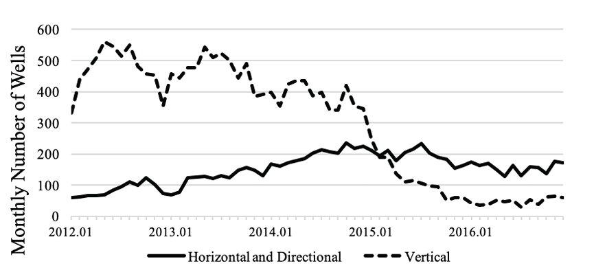
Source: data from Primary Vision.

Figure 2. Median reported water use of hydraulically fractured wells in the Permian Basin (January 2012 – December 2016).

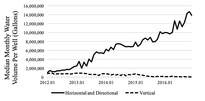
Source: data from Primary Vision.

Figure 3. Mean annual precipitation in Texas.

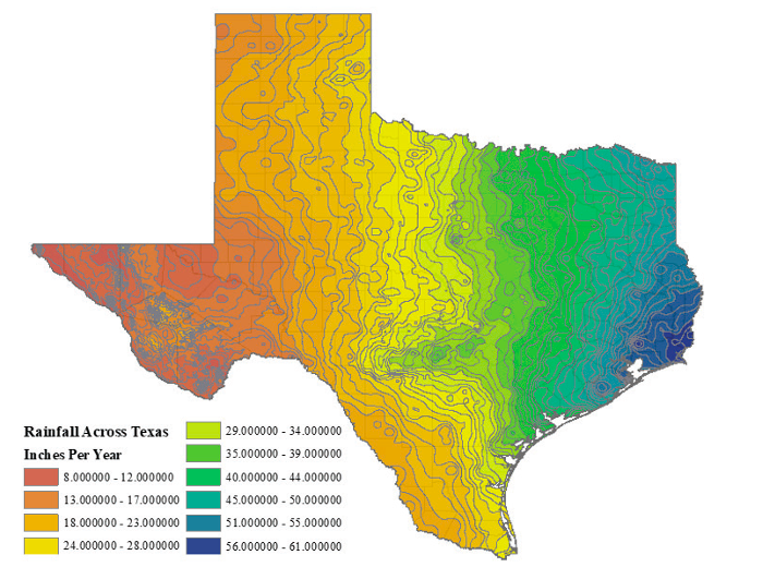
Figure created by author in ArcMap. Source: Texas rainfall shape file available at http://www.twdb.texas.gov/mapping/gisdata.asp.

Figure 4. Map of GCDs (in orange) in Texas. As of January 2019, there are 100 confirmed and 2 unconfirmed (pending election) GCDs in the state. The 100 confirmed GCDs cover 180 of the 254 counties in Texas.

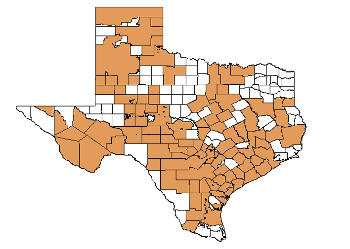
Figure created by author in ArcMap. Source: GCD shape file available at https://www.tceq.texas.gov/gis/download-tceq-gis-data.

Figure 5. Map of Texas counties, GCDs, and oil and gas well locations (in purple) across various unconventional plays.

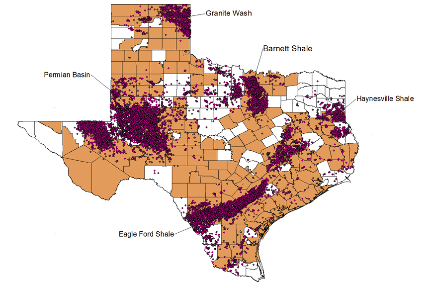
Figure created by author in ArcMap. Source: oil and gas well location data from Primary Vision.

Figure 6. Groundwater monitoring stations (blue dots) overlaying Texas counties, GCD areas, and oil and gas well locations (purple dots).

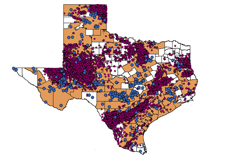
Figure created by author in ArcMap. Source: groundwater monitoring station locations obtained from the TWDB at https://www.waterdatafortexas.org/groundwater.

Figure 7. Operator reporting rates over time by area.

a) The percentage of well records for which Primary Vision estimated a hydraulic fracturing fluid mass in GCD and non-GCD areas.

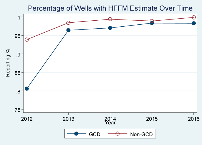
Source: data from Primary Vision.

b) The percentage of well records that contain at least some information on water type in GCD and non-GCD areas.

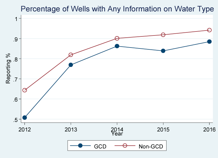
Source: data from Primary Vision.

Figure 8. Total water volumes used in hydraulic fracturing within the vicinity of a groundwater monitoring station. The thickness of the lines reflects the expected size of the effects of withdrawals across space.

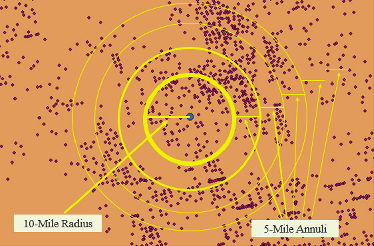
Figure created by author in ArcMap. Source: oil and gas well location data from Primary Vision.

Figure 9. Coefficient plot of the effects of water use in hydraulic fracturing across space. Estimates from equation (2). Each point is presented with its 95% confidence interval. Regression results are available in Appendix D.2A.

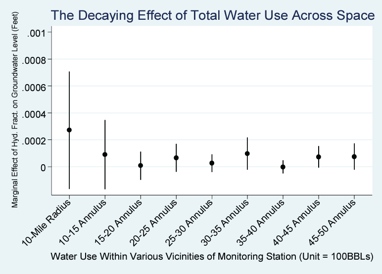
Source: data from Primary Vision.

Tables

Table 1. FracFocus disclosure requirements for Texas.

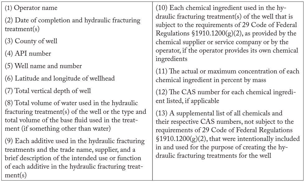
Source: House Bill 3328, Texas Legislature.

Table 2. Descriptive statistics. Median reported water volume (gallons) for all well records in GCD and non-GCD areas over January 2012 through May 2017. Statistics based on reported water volumes from well records in the PV dataset.

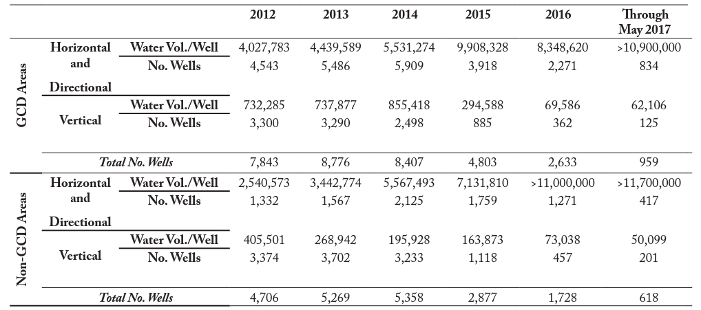
Source: data from Primary Vision.

Table 3. Linear probability model results for reporting metric 1. Outcome: hydraulic fracturing fluid mass calculated (0 or 1)? Each specification was estimated using wells in Texas over February 2012 through May 2017, but omitting observations for operators who did not have wells in both GCD and non-GCD areas.

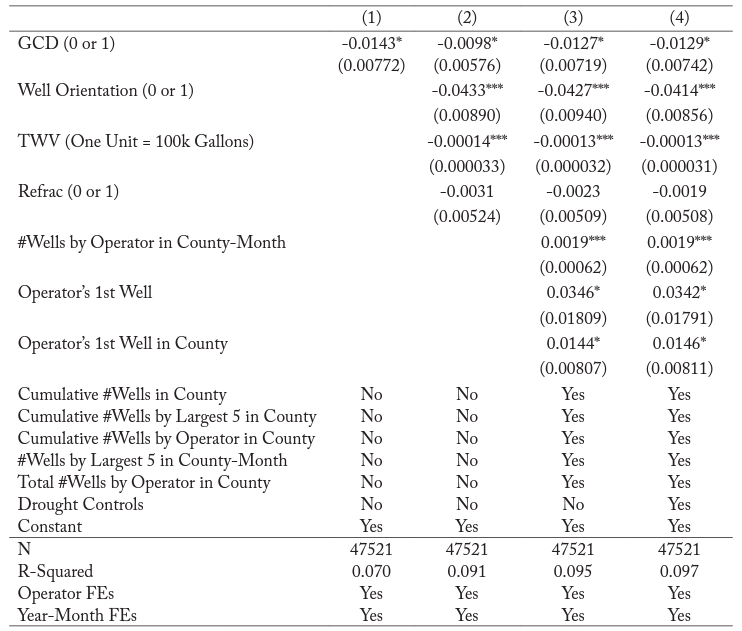
Standard errors in parentheses. Clustered on county. * p<0.10, ** p<0.05, *** p<0.01

Table 4. Linear probability model results for reporting metric 2. Outcome: any information on water type in completion report (0 or 1)? Each specification was estimated using wells in Texas over February 2012 through May 2017, but omitting observations for operators who did not have wells in both GCD and non-GCD areas.

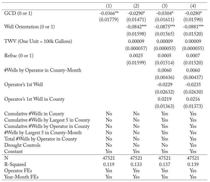
Standard errors in parentheses. Clustered on county. * p<0.10, ** p<0.05, *** p<0.01

Table 5. Naïve fixed effects model results. Outcome: distance to groundwater level (feet). Units of TWV are in 100BBLs (4,200 gallons).

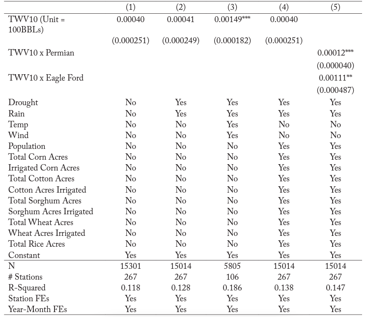
Standard errors in parentheses. Clustered on monitoring station. * p<0.10, ** p<0.05, *** p<0.01

Table 6. Fixed effects model results with lags for the short-term effects of water use in hydraulic fracturing. Lags indicated by (-). Outcome: distance to groundwater level (feet).

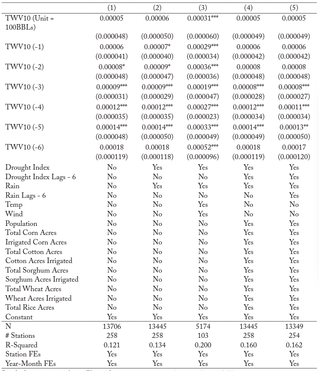
“Standard errors in parentheses. Clustered on monitoring station. * p<0.10, ** p<0.05, *** p<0.01

Table 7. Fixed effects model results for the cumulative effects of water use in hydraulic fracturing. Outcome: distance to groundwater level (feet).

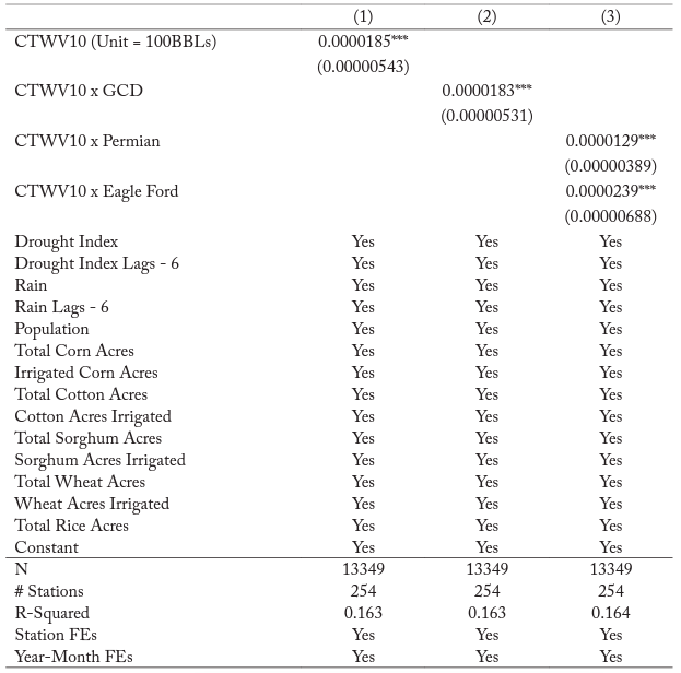
Standard errors in parentheses. Clustered on monitoring station. * p<0.10, ** p<0.05, *** p<0.01

References

Abramov, A. 2016. “Crude, Condensate Output Refuse to Decline; Average Well Configuration, Productivity Continue to Grow.” Oil & Gas Financial Journal Back Issues. Available at: https://www.ogj.com/articles/ogfj/print/volume-13/issue-5/features/permian-basin.html. [Accessed 7/19/17].

Agerton, M. 2019. “Learning Where to Drill: Drilling Decisions and Geological Quality in the Haynesville Shale.” Working Paper. Available at: http://markagerton.com/files/Agerton_LearningWhereToDrill.pdf. [Accessed 4/14/19].

Allen, W.T., R.D. Lacewell, and M. Zinn. 2014. “Water Value and Environmental Implications of Hydraulic Fracturing: Eagle-Ford Shale.” Texas Water Resources Institute Paper TR-466. Available at: https://oaktrust.library.tamu.edu/bitstream/handle/1969.1/152429/TR-466%20Water%20Value%20and%20Environmental%20Implications%20of%20Hydraulic%20Fracturing.pdf?sequence=1&isAllowed=y. [Accessed 10/29/17].

Angrist, J., and J.-S. Pischke. 2009. Mostly Harmless Econometrics: An Empiricist’s Companion, 1st. ed. New Jersey: Princeton University Press.

Barth-Naftilan, E., N. Aloysius, and J.E. Saiers. 2015. “Spatial and Temporal Trends in Freshwater Appropriation for Natural Gas Development in Pennsylvania’s Marcellus Shale Play.” Geophysical Research Letters, 42: 6348–6356.

Bartik, A.W., J. Currie, M. Greenstone, and C.R. Knittel. 2017. “The Local Economic and Welfare Consequences of Hydraulic Fracturing.” NBER Working Paper 23060. Available at: http://www.nber.org/papers/w23060. [Accessed 9/28/18].

Black, K.J., S.J. McCoy, and J.G. Weber. 2017. “When Externalities Are Taxed: The Effects and Incidence of Pennsylvania’s Impact Fee on Shale Gas Wells.” Journal of the Association of Environmental and Resource Economists, 5(1): 107–153.

Boudet, H., C. Cake, D. Bugden, E. Maibach, C. Roser-Renouf, and A. Leiserowitz. 2014. “‘Fracking’ Controversy and Communication: Using National Survey Data to Understand Public Perceptions of Hydraulic Fracturing.” Energy Policy, 65: 57–67.

Boudet, H., D. Bugden, C. Zanocco, and E. Maibach. 2016. “The Effect of Industry Activities on Public Support for ‘Fracking.’” Environmental Politics, 25(4): 593–612.

Burnett, J.W. 2013. “Hydraulic Fracturing and U.S. Water Policy.” Global Water Forum Discussion Paper 1309. Available at: http://www.globalwaterforum.org/wp-content/uploads/2013/03/Hydraulic-fracturing-and-US-water-policy-GWF-1309.pdf. [Accessed 4/3/18].

Burnett, J.W. 2015. “Unconventional Oil and Gas Development: Economic, Environmental, and Policy Analysis.” Agricultural and Resource Economics Review, 44(2): 3–27.

Cavender, A.B. 2011. “Texas Law Requires Disclosure of Hydraulic Fracturing Chemicals as of February 1, 2012.” Available at: https://www.pillsburylaw.com/images/content/3/9/3903.pdf. [Accessed 6/8/17].

Carr, H. 2017. “Wipe Out! – How Will Permian E&Ps Dispose of All That Produced Water?” Daily Energy Post. Available at: https://rbnenergy.com/wipe-out-how-will-permian-eandps-dispose-of-allthat-produced-water. [Accessed 7/18/17].

Chatterji, A.K., and M.W. Toffel. 2010. “How Firms Respond to Being Rated.” Strategic Management Journal, 31: 917–945.

Chen, J., R. Knight, H.A. Zebker, and W.A. Shreuder. 2016. “Confined Aquifer Head Measurements and Storage Properties in the San Luis Valley, Colorado, from Spaceborne InSAR Observations.” Water Resources Research, 52: 3623–3636.

Conley, T.G., and F. Molinari. 2007. “Spatial Correlation Robust Inference with Errors in Location or Distance.” Journal of Econometrics, 14: 76–96.

Currie, J., M. Greenstone, and K. Meckel. 2017. “Hydraulic Fracturing and Infant Health: New Evidence from Pennsylvania.” Science Advances, 3(12): 1–9.

Doshi, A.R., G.W.S. Dowell, and M.W. Toffel. 2013. “How Firms Respond to Mandatory Information Disclosure.” Strategic Management Journal, 34: 1209–1231.

Ellsworth, W.L. 2013. “Injection-Induced Earthquakes.” Science, 341(6142): 1225942.

Estaville, L.E., and R.A. Earl. 2008. Texas Water Atlas, 1st ed. College Station: Texas A&M University Press.

Farah, N. 2017. “The Effects of Hydraulic Fracturing on Agricultural Productivity.” Working Paper. Available at: https://drive.google.com/file/d/0Bxp0L418FENjWklucjI3RzFvVkE/view. [Accessed 11/10/17].

Fetter, R.T. 2017. “Fracking, Toxics, and Disclosure.” Working Paper. Available at: https://sites.duke.edu/trfetter/files/2016/11/fracking-toxics-disclosure.pdf. [Accessed 3/15/18].

Fetter, R.T., A.L. Steck, C. Timmins, and D.H. Wrenn. 2018. “Learning by Viewing? Social Learning, Regulatory Disclosure, and Firm Productivity in Shale Gas.” NBER Working Paper No. 25401. Available at: https://www.nber.org/papers/w25401. [Accessed 1/20/19].

Feyrer, J., E.T. Mansur, and B. Sacerdote. 2017. “Geographic Dispersion of Economic Shocks: Evidence from the Fracking Revolution.” American Economic Review, 107(4): 1313–1334.

Fitzgerald, T. 2013. “Frackonomics: Some Economics of Hydraulic Fracturing.” Case Western Reserve Law Review, 63(4): 1337–1362.

Freyman, M. 2014. “Hydraulic Fracturing & Water Stress: Water Demand by the Numbers.” Shareholder, Lender, & Operator Guide to Water Sourcing—A Ceres Report. Available at: https://www.ceres.org/resources/reports/hydraulic-fracturing-water-stress-water-demand-numbers. [Accessed 6/15/17].

Gold, R. 2014. The Boom, 1st. ed. New York: Simon & Schuster.

Goldenberg, S. 2013. “A Texas Tragedy: Ample Oil, No Water.” Guardian. Available at: https://www.theguardian.com/environment/2013/aug/11/texas-tragedy-ample-oil-no-water. [Accessed 8/9/18].

Graham, J., J. Irving, X. Tang, S. Sellers, J. Crisp, Dhorwitz, L. Muehlenbachs, A. Krupnick, and D. Carey. 2015. “Increased Traffic Accident Rates Associated with Shale Gas Drilling in Pennsylvania.” Accident Analysis & Prevention, 74: 203–209.

Granger, C.W.J. 1969. “Investigating Causal Relations by Econometric Models and Cross-Spectral Methods.” Econometrica, 37(3): 424–438.

Hanson, G. 2011. “How Are Appropriate Water Sources for Hydraulic Fracturing Determined? Pre-Development Conditions and Management Phase Water Usage.” Louisiana State University Shreveport, as part of the proceedings of the Technical Workshops for the Hydraulic Fracturing Study: Water Resource Management, EPA. Available at: https://www.epa.gov/sites/production/files/documents/01a_Hanson_-_Appropriate_Water_Sources_508.pdf. [Accessed 10/8/18].

Hardberger, A. 2016. “Texas Groundwater Markets and the Edwards Aquifer: A Case Study for the Political Economy of Water Markets Project.” Unpublished, St. Mary’s University School of Law. Available at: https://static1.squarespace.com/static/56d1e36d59827e6585c0b336/t/5805468415d5dbb1ab59a3a9/1476740751543/Texas-Groundwater-Markets-Hardberger.pdf. [Accessed 8/15/17].

Hausman, C., and R. Kellogg. 2015. “Welfare and Distributional Implications of Shale Gas.” Brookings Papers on Economic Activity, 46(1): 71–139.

He, X., N. Lu, and R.P. Berrens. 2017. “The Case of the Missing Negative Externality? Housing Market Effects of Fracking in the Niobrara Shale Play, Colorado.” Journal of Environmental Economics and Policy, 7(3): 223–243.

Herrnstadt, E., R. Kellogg, and E. Lewis. 2019. “Information Asymmetry, Drilling Distortions, and Oil and Gas Leases.” Working Paper. Available at: https://home.uchicago.edu/~kelloggr/Papers/HKL_primaryterms.pdf. [Accessed 1/22/19].

Hill, E., and L. Ma. 2017. “Shale Development and Drinking Water Quality.” American Economic Review, 107(5): 522–525.

Hitaj, C., A. Boslett, and J.G. Weber. 2014. “Shale Development and Agriculture.” Choices, 29(4): 1–7.

Hitaj, C., A. Boslett, and J.G. Weber. 2017. “Fracking, Farming, and Water.” Working Paper. Available at: https://papers.ssrn.com/sol3/papers.cfm?abstract_id=3041868. [Accessed 9/28/18].

Holladay, J.S., and J. LaRiviere. 2017. “The Impact of Cheap Natural Gas on Marginal Emissions from Electricity Generation and Implications for Energy Policy.” Journal of Environmental Economics and Management, 85: 205–227.

Houston & Texas Central Railroad Co. v. W.A. East. 1904. 98 Tex. 146, 81 S.W. 279.

Horner, R.M., C.B. Harto, R.B. Jackson, E.R. Lowry, A.R. Brandt, T.W. Yeskoo, D.J. Murphy, and C.E. Clark. 2016. “Water Use and Management in the Bakken Shale Oil Play in North Dakota.” Environmental Science & Technology, 50: 3275–3282.

Howarth, R.W., A. Ingraffea, and T. Engelder. 2011. “Natural Gas: Should Fracking Stop?” Nature, 477: 271–275.

Hubert, M. and B. Bullock. 1999. “Senate Bill 1: The First Big and Bold Step Toward Meeting Texas’s Future Water Needs.” Texas Tech Law Review, 30: 53–70.

Jackson, R.B., A. Vengosh, J.W. Carey, R.J. Davies, T.H. Darrah, F. O’Sullivan, and G. Petron. 2014. “The Environmental Costs and Benefits of Fracking.” Annual Review of Environment and Resources, 39: 327–362.

James, A., and B. Smith. 2017. “There Will Be Blood: Crime Rates in Shale-Rich U.S. Counties.” Journal of Environmental Economics and Management, 84: 125–152.

Knittel, C.R., K. Metaxoglou, and A. Trindade. 2015. “Natural Gas Prices and Coal Displacement: Evidence from Electricity Markets.” NBER Working Paper No. 21627.

Kondash, A.J., N.E. Lauer, and A. Vengosh. 2018. “The Intensification of the Water Footprint of Hydraulic Fracturing.” Science Advances, 4(8): 1–8.

Kondash, A., and A. Vengosh. 2015. “Water Footprint of Hydraulic Fracturing.” Environmental Science & Technology, 2: 276–280.

Konschnik, K., and A. Dayalu. 2015. “Hydraulic Fracturing Chemicals Reporting: Analysis of Available Data and Recommendations for Policymakers.” Energy Policy, 88: 504–514.

Krupnick, A.J. and H.G. Gordon. 2015. “What Experts Say About the Environmental Risks of Shale Gas Development.” Agricultural and Resource Economics Review, 44(2): 106–119.

Kusnetz, N. 2012. “The Bakken Oil Play Spurs a Booming Business—In Water.” High Country News. Available at: http://www.hcn.org/issues/44.13/the-bakken-oil-play-spurs-a-booming-business-inwater. [Accessed 6/4/17].

Kuwayama, Y., S. Olmstead, and A. Krupnick. 2015. “Water Quality and Quantity Impacts of Hydraulic Fracturing.” Current Sustainable Renewable Energy Reports, 2: 17–24.

Lange, I., and M. Redlinger. 2019. “Effects of Stricter Environmental Regulations on Resource Development.” Journal of Environmental Economics and Management, 96: 60–87.

Lesikar, B., R. Kaiser, and V. Silvy. 2002. “Questions About Groundwater Conservation Districts in Texas.” Texas A&M University Report. Available at: https://agrilifeextension.tamu.edu/library/water/questions-about-groundwater-conservation-districts-in-texas/. [Accessed 1/17/18].

Lin, Z., T. Lin, S.H. Lim, M.H. Hove, and W.M. Schuh. 2018. “Impact of Bakken Shale Development on Regional Water Uses and Supply.” Journal of the American Water Resources Association, 54(1): 225–239.

Lyon, T.P., and J.W. Maxwell. 2004. Corporate Environmentalism and Public Policy, Cambridge University Press.

Lyon, T.P., and J.W. Maxwell. 2008. “Corporate Social Responsibility and the Environment: A Theoretical Perspective.” Review of Environmental Economics and Policy, 2(2): 240–260.

Maniloff, P. 2019. “Can Learning Explain Deterrence? Evidence from Oil and Gas Production.” Journal of the Association of Environmental and Resource Economists, 6(5): 853–881.

Mason, C.F., L.A. Muehlenbachs, and S.M. Olmstead. 2015. “The Economics of Shale Gas Development.” Annual Review of Resource Economics, 7: 269–289.

Matisoff, D.C. 2013. “Different Rays of Sunlight: Understanding Information Disclosure and Carbon Transparency.” Energy Policy, 55: 579–592.

Mielke, E., L.D. Anadon, and V. Narayanamurti. 2010. “Water Consumption of Energy Resource Extraction, Processing, and Conversion.” Energy Technology Innovation Policy Research Group. Discussion Paper No. 2010–15. Belfer Center for Science and International Affairs, Harvard Kennedy School, Harvard University.

Mitchell, A.L., M. Small, and E.A. Casman. 2013. “Surface Water Withdrawals for Marcellus Shale Development: Performance of Alternative Regulatory Approaches in the Upper Ohio River Basin.” Environmental Science and Technology, 47(22): 12669–12678.

Muehlenbachs, L.A. 2012. “Testing for Avoidance of Environmental Obligations.” Resources for the Future Discussion Paper 12-12. Available at: https://ideas.repec.org/p/rff/dpaper/dp-12-12.html. [Accessed 6/11/19].

Muehlenbachs, L.A., and S. Olmstead. 2014. “Hydraulic Fracturing and Water Resources.” Choices, 29(4): 1–5. Muehlenbachs, L.A., E. Spiller, C. Timmins. 2015. “The Housing Market Impacts of Shale Gas Development.” American Economic Review, 105(12): 3633–3359.

Muehlenbachs, L.A., S. Staubli, and Z. Chu. 2017. “The Accident Externality from Trucking.” Resources for the Future Report. Available at: http://www.rff.org/research/publications/accident-externality-trucking. [Accessed 12/15/17].

Nicot, J.-P. 2012. “Current and Future Water Demand of the Texas Oil and Gas and Mining Sectors and Potential Impact on Aquifers.” GCAGS Journal, 1: 145–161.

Nicot, J.-P., and B.R. Scanlon. 2012. “Water Use for Shale-Gas Production in Texas, U.S.” Environmental Science & Technology, 46(6): 3580–3586.

Nicot, J.-P., R.C. Reedy, R.A. Costley, and Y. Huang. 2012. “Oil & Gas Water Use in Texas: Update to the 2011 Mining Water Use Report.” Austin, TX: Bureau of Economic Geology, University of Texas at Austin. Available at: http://www.twdb.texas.gov/publications/reports/contracted_reports/doc/0904830939_2012Update_MiningWaterUse.pdf. [Accessed 6/21/17].

Nicot, J.-P., B.R. Scanlon, R.C. Reedy, and C.A. Costley. 2014. “Source and Fate of Hydraulic Fracturing Water in the Barnett Shale: A Historical Perspective.” Environmental Science & Technology, 48(4): 2464–2471.

Olmstead, S.M., L.A. Muehlenbachs, J.-S. Shih, Z. Chu, and A.J. Krupnick. 2013. “Shale Gas Development Impacts on Surface Water Quality in Pennsylvania.” Proceedings of the National Academy of Sciences, 110(13): 4962–4967.

Olmstead, S.M., N. Richardson. 2014. “Managing the Risks of Shale Gas Development Using Innovative Legal and Regulatory Approaches.” William & Mary Environmental Law and Policy Review, 39(1): 177–199.

Provencher, B., and O. Burt. 1993. “The Externalities Associated with the Common Property Exploitation of Groundwater.” Journal of Environmental Economics and Management, 24: 139–158.

Rahm, D., B. Fields, B., and J.L. Farmer. 2015. “Transportation Impacts of Fracking in the Eagle Ford Shale Development in Rural South Texas: Perceptions of Local Government Officials.” The Journal of Rural and Community Development, 10(2): 78–99.

Rahm, B.G., and S.J. Riha. 2012. “Toward Strategic Management of Shale Gas Development: Regional, Collective Impacts on Water Resources.” Environmental Science & Policy, 17: 12–23.

Rahm, B.G., and S.J. Riha. 2014. “Evolving Shale Gas Management: Water Resource Risks, Impacts, and Lessons Learned.” Environmental Science Processes & Impacts, 16: 1400–1412.

Richey, S.R., B.F. Thomas, M.-H. Lo, J.T. Reager, J.S. Famigliette, K. Voss, S. Swenson, and M. Rodell. 2015. “Quantifying Renewable Groundwater Stress with GRACE.” Water Resources Research, 51: 5217–5238.

Scanlon, B.R., I. Duncan, and R.C. Reedy. 2013. “Drought and the Water-Energy Nexus in Texas.” Environmental Research Letters, 8: 1–14.

Scanlon, B.R., R.C. Reedy, and J.-P. Nicot. 2014a. “Comparison of Water Use for Hydraulic Fracturing for Unconventional Oil and Gas Versus Conventional Oil.” Environmental Science & Technology, 48: 12386–12393.

Scanlon, B.R., R.C. Reedy, and J.-P. Nicot. 2014b. “Will Water Scarcity in Semiarid Regions Limit Hydraulic Fracturing of Shale Plays?” Environmental Research Letters, 9(12): 1–14.

Scanlon, B.R., R.C. Reedy, F. Male, and M. Hove. 2016. “Managing the Increasing Water Footprint of Hydraulic Fracturing in the Bakken Play, United States.” Environmental Science & Technology, 50: 10273–10281.

Scanlon, B.R., R.C. Reedy, F. Male, and M. Welsh. 2017. “Water Issues Related to Transitioning from Conventional to Unconventional Oil Production in the Permian Basin.” Environmental Science & Policy, 51: 10903–10912.

Schafft, K.A., Y. Borlu, and L. Glenna. 2013. “The Relationship Between Shale Gas Development in Pennsylvania and Local Perceptions of Risk and Opportunity.” Rural Sociology, 78(2): 143–166.

Small, M.J., P.C Stern, E. Bomberg, S.M. Christopherson, B.D. Goldstein, A.L. Israel, R.B. Jackson, A. Krupnick, M.S. Mauter, J. Nash, D.W. North, S.M. Olmstead, A. Prakash, B. Rabe, N. Richardson, S. Tierney, T. Webler, G. Wong-Parodi, and B. Zielinska. 2014. “Risks and Risk Governance in Unconventional Shale Gas Development.” Environmental Science & Technology, 48(15): 8289–8297.

Smith, S.M. 2018. “Economics Incentives and Conservation: Crowding-In Social Norms in a Groundwater Commons.” Journal of Environmental Economics and Management, 90: 147–174.

Stepan, D.J., R.E. Shockey, B.A. Kurz, N.S. Kalenze, R.M. Cowan, J.J. Ziman, and J.A. Harju. 2010. “Bakken Water Opportunities Assessment—Phase 1.” Northern Great Plains Water Consortium. Prepared by the Energy & Environmental Research Center—University of North Dakota for the Industrial Commission of North Dakota. Available at: https://www.undeerc.org/water/pdf/FracWaterPhaseIreport.pdf. [Accessed 7/1/18].

Stevens, R.B., and G.L. Torell. 2018. “Exceptional Drought and Unconventional Energy Production.” Sustainability, 10(4): 1–16.

Street, B. 2018. “The Impact of Economic Opportunity on Criminal Behavior: Evidence from the Fracking Boom.” Working Paper. Available at: https://brittanystreet.github.io/website/Street_Brittany_jmp.pdf. [Accessed 4/29/19].

U.S. EPA. 2016. “Hydraulic Fracturing for Oil and Gas: Impacts from the Hydraulic Fracturing Water Cycle on Drinking Water Resources in the United States.” Final Report. Available at: https://cfpub.epa.gov/ncea/hfstudy/recordisplay.cfm?deid=332990. [Accessed 6/6/17].

U.S. Geological Survey (USGS). 2016. “Water Questions & Answers: How much water does the average person use at home per day?” Available at: https://water.usgs.gov/edu/qa-home-percapita.html. [Accessed 11/18/17].

Vengosh, A., R.B. Jackson, N. Warner, T.H. Darrah, and A. Kondash. 2014. “A Critical Review of the Risks to Water Resources from Unconventional Shale Gas Development and Hydraulic Fracturing in the United States.” Environmental Science & Technology, 48(15): 8334–8348.

Walsh, F.R., III, and M.D. Zoback. 2015. “Oklahoma’s Recent Earthquakes and Saltwater Disposal.” Science Advances, 1(5): e1500195.

Weber, J.G., and C. Hitaj. 2015. “What Can We Learn About Shale Gas Development from Land Values? Opportunities, Challenges, and Evidence from Texas and Pennsylvania.” Agricultural and Resource Economics Review, 44(2): 40–58.

Weber, J.G., J.W. Burnett, and I.M. Xiarchos. 2016. “Broadening Benefits from Natural Resource Extraction: Housing Values and Taxation of Natural Gas Wells as Property.” Journal of Policy Analysis and Management, 35(3): 587–614.

Executive Summary

Resources

Related Publications

Related News

Related Blogs

Focuses

States

Introduction

Literature Review

Background

Water Use in Oil and Gas

Texas Oil and Gas Water Markets — Informal and Formal

Groundwater Institutions in Texas

Common Law: Rule of Capture

Groundwater Conservation Districts

Senate Bill 1

Senate Bill 2 and A (Water) Data Problem

House Bill 3328

Data

Primary Vision

Other Controls and Data Manipulations

Groundwater Monitoring Stations

GCD Indicator

Weather Data

Other Data

Empirical Strategy

Reporting Water Use

Metrics for Reporting Water

Model Choices

The Causal Effects on Local Groundwater Levels

Naïve Approach

Alternative Approach

Cumulative Effects

Results

Strategic Reporting of Water Use

The Causal Effects of Hydraulic Fracturing on Groundwater Levels

Preliminary Spatial Evidence

The Short-Term Causal Effects

The Long-Term Causal Effects

Discussion

Conclusion

Figures

Tables

References