Reducing Misinformation on Social Media: An Experimental Evaluation of Two Policy Interventions

Samad, Zeeshan; Rentschler, Lucas

Introduction

Although misinformation is nothing new, the topic has gained prominence in recent years due to widespread circulation of entirely fabricated stories (presented as legitimate news) about broad-interest topics, such as the COVID-19 pandemic, election fraud, civil war, and foreign interference in US presidential elections. Misinformation is dangerous because it leads to inaccurate beliefs and creates partisan disagreements over basic facts. Given that social media has become a hub for misinformation and the fact that more than half of US adults get their news from social media (Shearer, 2021), tackling misinformation on social media is now more important than ever.

Researchers have developed a variety of policy recommendations that could reduce the amount of sharing and believing of misinformation on social media. Some of these recommendations include providing fact-checked information related to news articles (Lazer et al., 2018; Graves, 2016; Kriplean et al., 2014; Pennycook et al., 2020; Yaqub et al., 2020), nudging people to think about accuracy as they decide whether to share a news article on social media (Pennycook et al., 2021; Jahanbakhsh et al., 2021), increasing competition among media firms (Mullainathan and Shleifer, 2005; Blasco and Sobbrio, 2012; Gentzkow and Shapiro, 2008), and detecting false articles using machine learning algorithms (Tacchini et al., 2017; Wang, 2017).

In this study, we evaluate the effectiveness of two such policy interventions, namely competition among media firms and third-party fact-checking, on misinformation. We present a theoretical model that predicts how a rational media firm and news consumer would behave in a sequential game in which a media firm first chooses a costly action (e.g., how many journalists to hire) that determines the accuracy of the news it will produce. After a news article is published, a consumer decides whether or not to share this news article on social media. The consumer does not (yet) know if the news article is true or false but knows its probability of being true. The consumer gets a positive payoff if he shares a news article that turns out to be true and gets a negative payoff if he shares a news article that turns out to be false. The media firm receives a positive payoff if the consumer chooses to share its news article on social media and receives a zero payoff if the consumer does not share its news article on social media.

We implement this model at the Utah State University Experimental Economics Lab using a 2×2 design. In a base treatment, we ask subjects to play a two-player game in which a sender (who is meant to represent the media firm) first chooses an accuracy level between 50 and 100 percent such that higher accuracy levels cost more money. Based on that accuracy, the computer sends a true or false message to a receiver (who is meant to represent the news consumer). The higher the accuracy chosen by the sender, the more likely that the receiver sees a true message. The receiver observes the accuracy level and the message generated and then decides whether or not to affirm the message. If the receiver affirms, then he earns $10 if the message turns out to be true and loses $10 if the message turns out to be false. If the receiver does not affirm, his payoff is $0. The sender earns $10 if the receiver affirms or $0 if the receiver does not affirm.

To complete the 2×2 design, we add three more treatments, namely a competition treatment, a fact-checking treatment, and a competition plus fact-checking treatment. Each treatment involves exactly one modification to the game. In the competition treatment, we add another sender to the game so that the receiver now sees two messages and two accuracy levels and can affirm, at most, one of them. In the fact-checking treatment, all messages must go through a fact-checking process before being sent to the receiver. The fact-checking process lets true messages pass with certainty and lets false messages pass with a 75 percent chance—with the remaining a 25 percent chance, the false message is deleted and the sender is asked to choose a new accuracy, based on which a new message gets generated. In the competition plus fact-checking treatment, we combine both features mentioned above so that there are two senders and each sender’s message goes through the fact-checking process before being sent to the receiver.

We find that senders in the competition treatment choose a much higher accuracy, on average, than senders in the base treatment. Senders in the fact-checking treatment, however, do not choose any higher (or lower) accuracy than do senders in the base treatment. This finding suggests that, in this type of an environment, competition among media firms is highly effective at reducing misinformation, whereas fact-checking is not.

Model

We develop a sequential game played between a media firm and a news consumer. We first provide a motivating example to illustrate the type of situation this theoretical game attempts to simulate. Next, we describe the game and create multiple environments—where each environment is essentially a different game—to test the effects of specific policy interventions.

In a base environment, i.e., the game that is played in the absence of any policy intervention, a media firm decides how much money to invest toward increasing its news accuracy in the first stage. In the second stage, a news article gets published based on the accuracy chosen by the media firm, and a news consumer decides whether or not to share this article on social media. The consumer makes this decision knowing the probability that the article is true but without knowing whether it is actually true. The media firm is incentivized to invest the lowest amount at which the consumer would share the article on social media, and the consumer is incentivized to share a true article and is disincentivized to share a false article. We develop two more games that are slight modifications of the base environment to capture the effect of two policy interventions.

To evaluate the effect of media competition on equilibrium outcomes, we develop another game, namely a competition environment, in which we add another media firm and let the two firms and one consumer play a three-player sequential game. In this environment, both firms simultaneously choose their investments in accuracy in the first stage. In the second stage, the news consumer decides which firm’s article, if any, to share on social media. We then develop a fact-checking environment, wherein we modify the base environment by adding an exogenous fact-checker, played by Nature for the purposes of the game. This fact-checker plays after the firm chooses its investment and a news article gets published but before the consumer learns that an article has been published. The fact-checker either deletes the article or allows the article to pass. More precisely, if the published news article is true, the fact-checker allows the article to pass and lets the consumer learn about it, but if it is false, then there is a 25 percent chance that the fact-checker deletes it—in which case the firm must make a new investment and publish a new article—and a 75 percent chance that the fact-checker lets the article pass and reach the consumer. The consumer, who does not know whether she is seeing the first or second (or nth) article published by the firm, decides, as before, whether or not to share the article on social media.

Base Environment

Setup

There are two players, a sender ( $S$ ) and a receiver ( $R$ ), and a state of the world that can be either red or blue, $w\in\{red,blue\}$ . It is common knowledge that either state has an equal likelihood of occurring; i.e., $Pr(blue) = Pr(red) = 0.5$ . However, neither player knows the actual realization of $w$ . A message, $m\in \{red,blue\}$ , informs the receiver about the realized state of the world. We define accuracy ( $q$ ) of the message $m$ as the probability with which the message is correct given the state of the world. That is, $\text{Pr}(m=w)=q$ and $\text{Pr}(m \neq w)=1-q$ . In other words, $m|w\sim Ber(q)$ .

The game is played in two stages. In the first stage, the sender chooses $q\in[0.5,1]$ . In the second stage, the receiver observes $q$ and the realization of $m$ and then decides whether or not to affirm the message, a decision denoted by $a\in \{0,1\}$ . The sender also has to pay an accuracy cost that is determined by an increasing convex function $c(q)$ that has the following properties: $c^{\prime} (q)>0, c^{\prime\prime} (q)>0$ , and $c(0.5)=0$ . The last property implies that a completely uninformative message requires zero investment. The sender pays this accuracy cost at the time of choosing an accuracy level, so this cost is incurred even if the receiver does not affirm the message.

The sender’s payoff is entirely dependent on the receiver’s action. If the receiver affirms the message, the sender earns a high payoff that we normalize to $1, resulting in a net payoff of $1-c(q)$ . If the receiver does not affirm the message, the sender earns a low payoff of $0.5, resulting in a net payoff of $0.5 − c(q)$ . The receiver’s payoff depends on his own action as well on whether the message is true. If the receiver affirms the message and the message is true, then the receiver’s payoff is $1. If the receiver affirms the message and the message is false, then the receiver’s payoff is zero (although the sender would still earn $1 in this case). If the receiver does not affirm the message, the receiver’s payoff is 0.5. Figure 1 presents the extensive form of this game.

Figure 1. Illustration of Base Environment

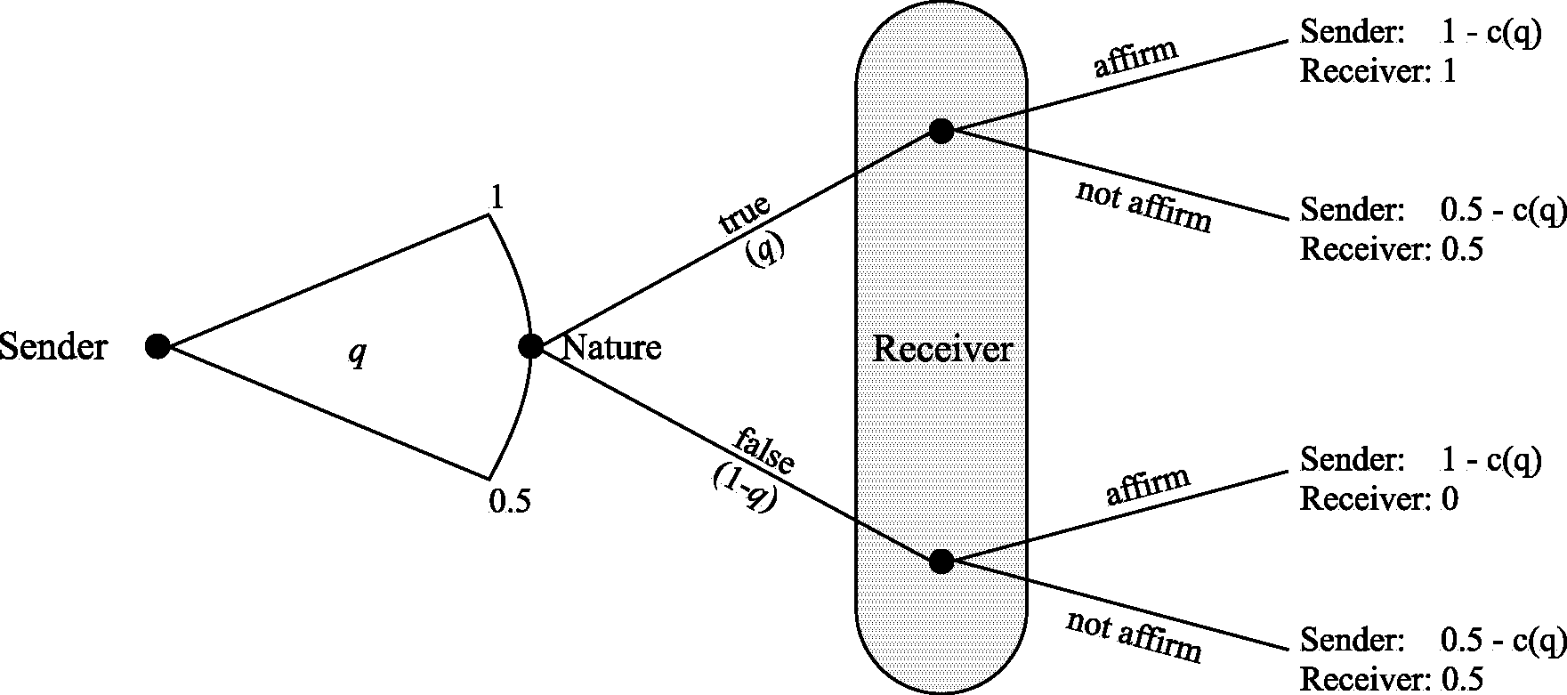
To focus on nontrivial cases, we make two further assumptions. First, $c(1)=0.5$ so that the cost of sending a 100 percent accurate message is so high that it nullifies any additional payoff from the receiver affirming the message. Second, we assume that the sender’s utility function is linear, while the receiver’s utility function is concave.¹ Specifically, the sender’s and the receiver’s utility functions are

$U_S (q;a) = \begin{cases} 1 - c(q) & \text{if } a=1 \\ 0.5 - c(q) & \text{if } a=0, \end{cases}$

$U_R (a;m(q),w) = \begin{cases} v(1) &\text{if } a=1 \text{ and } m=w \\ v(0) &\text{if } a=1 \text{ and } m \neq w \\ v(0.5) & \text{if } a=0, \end{cases}$

where $v(x)$ is a continuous function such that $v^\prime (x) > 0$ , $v^{\prime \prime} (x) < 0$ , and $v(0)=0$ . Given that $\text{Pr}(m=w)=q$ , the receiver’s expected utility from affirming is $\mathbb{E}U_R(a=1)= q v(1) + (1-q)v(0)$ .

Note that while the sender is risk neutral in his overall wealth, he is still risk averse in $q$ because $c(q)$ is convex. That is, $U_S(\pi)$ is linear, while $U_S(q)$ is concave.

Equilibrium

To arrive at the subgame perfect Nash equilibrium (SPNE), we solve the game through backward induction, first deriving the receiver’s optimal strategy given $q$ and then deriving the sender’s best response to the receiver’s strategy. Proposition 1 provides the receiver’s optimal strategy. All proofs are in Appendix A.

Proposition 1.

(i) There exists a unique $q^B\in (0.5,1)$ s.t. $\mathbb{E}U_R (a=1) = U_R (a=0)$ .
(ii) The receiver’s optimal strategy is $a(q) =

$\begin{cases} 1 &\text{if } q\geq q^B \\ 0 &\text{if } q < q^B. \end{cases}$$

Proposition 1 states that there is some threshold value of $q^B$ such that the receiver finds it profitable to affirm the message for accuracy levels greater than $q^B$ and finds it not profitable for accuracy levels less than $q^B$ . Intuitively, if the sender chooses $q=1$ , then there would be no risk involved, and therefore any risk-averse receiver would strictly prefer to affirm. On the other extreme, if the sender chooses $q=0.5$ , then no receiver would want to affirm. Somewhere in between these two extremes, there has to be a point where the receiver is indifferent between affirming and not affirming.

Proposition 2. The sender’s optimal strategy is $q=q^B$ , resulting in the following SPNE:

$\begin{pmatrix} q^B\\ \mathds{1}\cdot (q\geq q^B) \end{pmatrix}$

Proposition 2 states that the sender will choose the minimum accuracy level that he believes will get the message affirmed. For further illustration, we provide some examples in Appendix A that highlight the differences in each environment.

Competition Environment

Setup

We construct a competition environment by adding another sender to the game presented in the base environment, which results in a new game played between three players: Sender 1 ( $\(S_1$ ), Sender 2 ( $\(S_2$ ), and Receiver ( $R$ ). As before, the game is played in two stages. In the first stage, each sender $S_i$ , for $i\in\{1,2\}$ , simultaneously and independently chooses $q_i\in[0.5,1]$ and incurs a cost of $c(q_i)$ . In the second stage, the receiver observes $q_1$ and $q_2$ along with realizations of $m_1$ and $m_2$ , where $m_i \in \{\hat{r},\hat{b}\} \sim Ber(q_i)$ , for $i\in\{1,2\}$ . The receiver’s choice is denoted by $a\in\{0,1,2\}$ , where $a=1$ represents the decision to affirm $m_1$ , $a=2$ represents the decision to affirm $m_2$ , and $a=0$ represents the decision to affirm neither message. Players’ payoffs are as follows:

$U_{S_i} (q_i;a) = \begin{cases} 1 - c(q_i) & \text{if } a=i \\ 0.5 - c(q_i) & \text{if } a \neq i, \end{cases}$

$U_R (a;m_i,w) = \begin{cases} v(1) &\text{if } a= i \text{ and } m_i=w \\ v(0) &\text{if } a= i \text{ and } m_i \neq w \\ v(0.5) &\text{if } a=0. \end{cases}$

Equilibrium

We first derive the receiver’s optimal strategy.

Proposition 3. The receiver’s optimal strategy is

$a= \begin{cases} 0 &\text{if } q_1 < q^B \text{ and } q_2 < q^B \\ 1 &\text{if } q_1 > q_2 \text{ and } q_1 \geq q^B \\ 2 &\text{if } q_2 > q_1 \text{ and } q_2 \geq q^B \\ 1 \text{ or } 2 &\text{if } q_1 = q_2 \geq q^B. \end{cases}$

Proposition 3 states that the receiver will affirm the message that has a higher accuracy as long as that accuracy is greater than his threshold of $q^B$ . If both messages have the same accuracy and that accuracy is greater than $q^B$ , then the receiver is indifferent between affirming either of the two messages and resolves this indifference by randomly choosing one message.

Next, we derive the optimal strategy for each sender. The senders in this environment are essentially bidders in a first price all-pay auction (FPAA) because sender $S_i$ “bids” $c(q_i)$ and pays this bid regardless of which message gets affirmed. The “winning” sender receives an additional payoff of $0.5. Therefore, to determine each sender’s optimal strategy, we apply the equilibrium of an FPAA with convex costs and a reservation price of $q^B$ .²

Proposition 4. There is a symmetric equilibrium in which each sender continuously randomizes over the range $q \in [q^B,1]$ using the distribution function $F(q) = 2c(q)$ .

Proposition 4 states that senders play a mixed strategy over the continuous range $[q^B,1]$ and choose probabilities according to the distribution $F(q)$ . Example 2 (in Appendix A) presents a numerical example of the equilibrium in this environment.

Fact-Checking Environment

Setup

We construct a fact-checking environment by modifying the base environment to include a fact-checking process. As in the base environment, the sender chooses an accuracy level and the computer chooses the true message with that much probability. However, before the message is shown to the receiver, it gets randomly selected, with a 25 percent chance, of getting checked.³ A message that gets checked either proceeds as normal or gets deleted, depending on whether it is true or false. If a message is false, then it gets deleted and the sender is asked to choose a new accuracy, based on which a new message is randomly chosen. While the receiver is aware of the fact-checking process, he cannot tell whether the message he sees got checked.

The sender faces a game that could potentially (although with near-zero probability) go on forever. This is because with a probability of $0.25(1-q)$ , the message will get deleted and the sender will be asked to choose a new accuracy. With the remaining probability, $1-0.25(1-q)$ , the message passes through the fact-checking process and goes to the receiver.

In the event that a message gets deleted, the sender would face the exact same game that he faced earlier: he would need to choose an accuracy $q\in [0.5,1]$ , and the new message would have the same probability of clearing the fact-checking process. Therefore, the sender’s optimal choice of $q$ would remain the same each time he is asked regardless of how many previous messages got deleted.

In this environment, the sender’s utility function is

$U_S (q;a) = \begin{cases} 1 -\mathbb{E}[c (q)] & \text{if } a=1 \\ 0.5 - \mathbb{E}[c (q)] & \text{if } a =0, \end{cases}$

where, assuming the sender chooses the same accuracy each time he is asked,

$\begin{align*} \mathbb{E}[c (q)] &= c(q) + (0.25)(1-q)c(q) + (0.25)^2(1-q)^2 c(q) + ... \\ &= \frac{c(q)}{0.75 + 0.25q}. \end{align*}$

The receiver’s utility function is the same as in the base environment; i.e.,

$U_R (a;m(q),w) = \begin{cases} v(1) &\text{if } a=1 \text{ and } m=w \\ v(0) &\text{if } a=1 \text{ and } m \neq w \\ v(0.5) & \text{if } a=0. \end{cases}$

Equilibrium

Since some messages get deleted, the mere fact that the receiver sees a message tells the receiver that it is not among those that got deleted. The receiver would be interested in the effective probability that the message is true, i.e., the probability that a message is true conditional on the fact that it gets seen by the receiver. We can derive this using Bayes’ rule, as follows:

$\begin{align*} \text{Pr(true|seen)} &= \frac{\text{Pr(seen|true)Pr(true)}}{\text{Pr(seen|true)Pr(true)+ Pr(seen|false)Pr(false)}} \\ &= \frac{q}{q + 0.75(1-q) } \\ &= \frac{q}{0.75+0.25q}. \end{align*}$

The receiver finds it optimal to affirm as long as this probability is greater than his threshold accuracy of $q^B$ (see Proposition 1); i.e.,

$a= \begin{cases} 0 &\text{if } \frac{q}{0.75+0.25q} < q^B \\ 1 &\text{if } \frac{q}{0.75+0.25q} \geq q^B. \end{cases}$

Simplifying this results in

$a= \begin{cases} 0 &\text{if } q < q^F \\ 1 &\text{if } q \geq q^F \end{cases} \hspace{0.2em} \text{, where } q^F = \frac{3q^B}{4-q^B}.$

As in the base environment, the sender’s best response is to choose the lowest accuracy at which the receiver would affirm (see Proposition 2), resulting in the SPNE $\{q^F, \mathds{1}\cdot (q\geq q^F) \}$ . Perhaps unsurprisingly, senders end up choosing a lower accuracy level in the fact-checking environment than they do in the base environment; i.e., $q^F \leq q^B$ . Intuitively, this is because the fact-checking process improves the overall accuracy of messages seen by the receiver, allowing the sender to now get away with a lower accuracy.

Competition and Fact-Checking Environment

Setup

Last, we construct a competition and fact-checking environment by adding both modifications, i.e., fact-checking and competition, to the base environment. In this environment, there are two senders who simultaneously choose their respective accuracy levels. Each sender’s message gets selected for fact-checking with a probability of 0.25. When both senders’ messages successfully go through the fact-checking process explained earlier, the receiver sees both messages along with the accuracy of each message. If a message gets deleted during the fact-checking process, only the sender whose message it is gets informed about it.

In this environment, for $i\in \{1,2\}$ , Sender i’s utility function is

$U_{S_i} (q_i;a) = \begin{cases} 1 -\mathbb{E}[c (q_i)] & \text{if } a=i \\ 0.5 - \mathbb{E}[c (q_i)] & \text{if } a \neq i, \end{cases}$

where

$\begin{align*} \mathbb{E}[c (q_i)] &= c(q_i) + (0.25)(1-q_i)c(q_i) + (0.25)^2(1-q_i)^2 c(q_i) + ... \\ &= \frac{c(q_i)}{0.75 + 0.25q_i}. \end{align*}$

The receiver’s utility is

$U_R (a;m_i,w) = \begin{cases} v(1) &\text{if } a= i \text{ and } m_i=w \\ v(0) &\text{if } a= i \text{ and } m_i \neq w \\ v(0.5) &\text{if } a=0. \end{cases}$

The receiver’s expected utility from affirming message $i\in\{1,2\}$ is

$\mathbb{E}U_R (a=i)= \widetilde{q_i} v(1) + (1-\widetilde{q_i})v(0),$

where $\widetilde{q_i} = \text{Pr(true|seen)} = \frac{q_i}{0.75+0.25q_i}$ .

Equilibrium

The receiver’s optimal strategy is

$a= \begin{cases} 0 &\text{if } q_1,q_2 < q^F \\ 1 &\text{if } q_1 \geq q_2 \text{ and } q_1 \geq q^F \\ 2 &\text{if } q_1 \leq q_2 \text{ and } q_2 \geq q^F. \\ \end{cases}$

That is, the receiver will affirm the message that has the higher accuracy as long as that accuracy is at least as much as $q^F$ .

Each sender’s best response is to continuously randomize with $F(q) = 2c(q)$ over the support $[q^F,1]$ —a straightforward extension of Proposition 4.

Summary of Results and Testable Hypotheses

The environments described earlier are designed specifically to evaluate the impact of media competition and fact-checking on the amount of misinformation shared on social media. All environments simulate situations where media firms decide how much money to invest toward increasing their news accuracy, and news consumers decide whether or not to share the firm’s news article on social media. That is, $q$ represents news accuracy, while $c(q)$ represents the amount invested by the firm toward news accuracy.

Table 1 summarizes the Nash equilibrium strategies in all four environments.

Table 1. Equilibrium Predictions

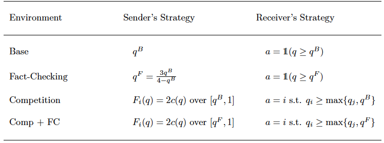
Our theoretical predictions lead to the following testable hypotheses.

Hypothesis 1. Of the four environments described earlier, the competition environment creates the strongest incentive for firms to invest in accuracy.

In the base and fact-checking environments of our model, where the sender has a monopoly position, the sender chooses the lowest accuracy at which the receiver would be willing to affirm the message. These accuracy levels are $q^B$ and $q^F$ for the base and fact-checking environments, respectively, with $q^F<q^B$ . In the other environments, where there are two senders, each sender’s best response is to continuously randomize over some range $[q,1]$ using some probability distribution function $f(q)$ . In the competition environment, the average accuracy level chosen by senders is $q^C= E[q]=\int^1_{q^B} qf(q)dq$ , whereas in the competition plus fact-checking environment, it is $q^{CF}= E[q]=\int^1_{q^F} qf(q)dq$ . Given that $q^F<q^B$ , this results in $q^{CF} < q^C$ . Therefore, the (average) accuracy levels chosen by firms in all four environments can be ranked as follows:

$q^F < q^B < q^{CF} < q^C.$

Hypothesis 2. Holding accuracy levels constant, the presence of fact-checking makes consumers more likely to share a news article on social media.

The proportion of messages that receivers affirm is meant to represent the proportion of news articles that consumers share on social media. If senders do not play their Nash equilibrium strategy and instead randomly choose a value of $q\in[0.5,1]$ , then the proportion of messages that will be affirmed by the receiver would be greater in the presence of fact-checking.

Specifically, let $q$ be a random variable with c.d.f. $F_q$ s.t. $F_q(0.5)=0$ and $F_q(1)=1$ . In the base environment, the receiver’s likelihood of affirming would be $1-F(q^B)$ . In the fact-checking environment, this would be $1-F(q^F)$ , which is greater than $1-F(q^B)$ . Similarly, the receiver’s likelihood of affirming a message would be $1-[F(q^B)]^2$ in the competition environment and $1-[F(q^F)]^2$ in the competition and fact-checking environment.

Experiment Design

We now explain our experimental procedures and treatment designs. We develop four experimental treatments, each of which implements one of the environments described in the model section. We call these the base treatment, competition treatment, fact-checking treatment, and competition plus fact-checking treatment. Given that each treatment is different from another in terms of only one feature, a comparison across these four treatments gives us a clean and robust way to evaluate the effect of that single feature and allow us to answer several important policy questions. For example, does media competition incentivize firms to improve accuracy of their news? What about fact-checking? Moreover, do these interventions interact with one another or are their effects entirely independent?

Experimental Procedures

We conducted this experiment at the Experimental Economics Laboratory at Utah State University in Spring 2022. All subjects were university students and were recruited using Sona Systems.⁴ We recruited 201 subjects, who were divided across treatments as follows: 52 subjects participated in the base treatment, 51 in the competition treatment, 50 in the fact-checking treatment, and the remaining 48 in the competition plus fact-checking treatment.⁵ We conducted these four treatments over 13 sessions (four sessions for the fact-checking treatment and three sessions for each of the other treatments). All interaction between subjects took place anonymously through computers, and the experiment was coded using oTree (Chen et al., 2016). All subjects received a $7 show-up fee in addition to their earnings from the experiment. Each session took approximately 45 minutes, and average subject earnings were $21, including the show-up fee.

At the start of a session, subjects were asked to take a seat in a computer lab and were provided instructions and guidance by the software. First, subjects were asked to read through a detailed description of a game and were given an opportunity to ask questions. Next, they played an unpaid practice round in which they played as both the sender and the receiver. After the practice round, subjects were required to answer some understanding questions based on their choices in the practice round. They could only proceed to the main experiment upon answering all questions correctly.

After demonstrating good understanding of the game, subjects played 20 rounds of a sender-receiver game. At the end, one these rounds was randomly selected for payment. In each round, subjects were randomly reassigned the role of a sender or receiver and were randomly re-matched with another participant. Thus, we obtained 1,680 unique sender-receiver interactions for across the four treatments.⁶

After playing these 20 rounds, subjects were asked to complete a questionnaire that elicited their demographic information as well as their social preferences, specifically their preferences for risk, time, altruism, trust, and reciprocity preferences. To elicit these social preferences, we used questions from the Global Preferences Survey (Falk et al., 2018). However, instead of using their sequence of hypothetical questions about choosing between an uncertain option and a certain option, we asked them to participate in an incentivized and paid bomb risk elicitation task (Crosetto and Filippin, 2013). In this task, subjects are incentivized to collect a greater number of boxes, but the more boxes they collect, the greater the chance that they might lose all their earnings.⁷ The demographic questions collected information related to subjects’ age, gender, race, education, income, and religiousness.

The experiment instructions, round screenshots, and questionnaire are all provided in Appendix C.

Description of Treatments

Base Treatment

A sender and a receiver are endowed with $10 each. A ball is drawn at random from an urn that contains one red ball and one blue ball. Neither player observes the color of the ball drawn. A message, which can be either “the ball is red” or “the ball is blue,” is said to be true if it correctly states the color of the ball drawn and is false otherwise. In the first stage of the game, the sender chooses $q\in [0.5,1]$ and pays a cost of $c(q)=10(2q-1)^2$ . Based on this choice, the computer chooses a message to send to the receiver. Specifically, it chooses the true message with a probability of $q$ and the false message with a probability of $1 − q$ . In the second stage, the receiver sees the message chosen by the computer along with its probability of being true ( $q$ ). In other words, the receiver knows the probability with which the message is true but not if the message is actually true. The receiver is asked to either affirm or not affirm this message. He earns $10 if he affirms a true message, loses $10 if he affirms a false message, and earns nothing if he does not affirm the message. The sender earns $10 if the receiver affirms the message irrespective of whether it is true or false.

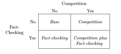
Additional Treatments. We develop a 2×2 factorial design to evaluate the impact of two policy interventions: media competition and third-party fact-checking. To vary competition, we include a treatment with two senders. To vary fact-checking, we include a treatment in which a bot randomly picks about one in four messages en route from the sender to the receiver and checks that message for accuracy; if the message is false, the bot removes it, and if the message is true, the both lets it proceed. Last, to check for any possible interaction between these two interventions, we include a treatment with two senders and a fact-checking bot. As table 2 illustrates, this results in a total of four treatments. We describe each treatment in more detail below. The complete instructions provided to the subjects are available in Appendix C.

Table 2. 2×2 Experimental Treatments

Competition Treatment

The only change in the competition treatment relative to the base treatment is that the number of senders is increased from one to two. Thus, this becomes a three-player game played over two stages. In the first stage, both senders choose, simultaneously and independently, the accuracy of their respective messages, $q_1$ and $q_2$ . Both senders face the same cost function, $c(q)=10(2q-1)^2$ . In the second stage, the receiver sees two messages, one from each sender, along with the accuracy of each message, and decides which, if any, of the two messages to affirm. That is, the receiver may affirm at most one message. The sender whose message is affirmed earns $10. The receiver, as before, earns $10 if he affirms a true message, loses $10 if he affirms a false message, and earns nothing if he chooses not to affirm either of the two messages.

Fact-Checking Treatment

The fact-checking treatment consists of one sender and one receiver. The only difference between the base treatment and the fact-checking treatment is that messages have a 25 percent chance of getting fact-checked, i.e., checked for their veracity, before being shown to the receiver. The first stage of the game is no different from the base treatment. That is, the sender chooses an accuracy, $q$ , based on which a message is generated (the true message is chosen with a probability of $q$ and the false message is chosen with the remaining probability of $1 − q$ ).

After a message is generated, there is an independent 25 percent chance that the message will get selected for fact-checking.⁸ If it gets selected, it is essentially deleted if it is false, and the sender is asked to choose a new accuracy. The computer then generates a new message based on that accuracy, and the new message also has a 25 percent chance of getting selected for fact-checking. If the message does not get selected for fact-checking or if the message is true, then it is shown to the receiver, who decides whether or not to affirm the message. As in the base treatment, the receiver earns $10 for affirming a true message, loses $10 for affirming a false message, and earns nothing if he does not affirm. The sender earns $10 if the receiver affirms the message, irrespective of whether it is true or false. If the sender is asked to choose an accuracy multiple times, she incurs the cost of all of her accuracy choices.

Comparing subjects’ decisions in this treatment with those in the base treatment allows us to estimate the effect of third-party fact-checking on both sides of the market. On the production side, we can check if the presence of fact-checking influences firms’ decisions to invest in quality. On the consumption side, we can test if fact-checking makes consumers feel more confident about sharing a news article on social media.

Competition Plus Fact-Checking Treatment

To complete the 2×2 design, we include a competition plus fact-checking treatment that contains both interventions. The main purpose of this treatment is to check if the two policies interact with one other. Specifically, if both policy interventions take place and the net effect is different from the sum of the individual treatment effects, then there is an interaction.

This treatment consists of two senders and one receiver. In the first stage, both senders simultaneously choose their respective accuracy levels, $q_1$ and $q_2$ . In the second stage, the computer generates two messages, one for each sender. Each message has a 25 percent chance of getting selected for fact-checking. If a message gets selected and turns out to be false, then it gets deleted and the sender of that message is notified and asked to choose a new accuracy. In this case, only the affected sender goes back to the first stage. If a message does not get selected for fact-checking or it gets selected but is true, then it is said to clear the fact-checking process.

When both messages clear the fact-checking process, the game proceeds to the third stage. In this stage, both messages are shown to the receiver and the receiver is asked to choose one of three options: (i) affirm Sender 1’s message, (ii) affirm Second 2’s message, or (iii) affirm neither message. If the receiver affirms a message, then he either earns an additional $10 or loses his current $10, depending on whether the message is true or false. If he does not affirm either message, he gets to keep his $10 endowment but does not have the opportunity to earn more. If the receiver affirms a message, then the sender whose message gets affirmed earns another $10 as well.

Results

Data

Our final data consist of 1,680 unique sender-receiver interactions that took place among 201 subjects over four treatments. These interactions are distributed as follows: 520 interactions in the base treatment, 500 in the fact-checking treatment, 340 in the competition treatment, and 320 in the competition plus fact-checking treatment. Despite having approximately the same number of subjects in each treatment, we observe fewer interactions in the latter two treatments because each interaction consists of three people, two senders and one receiver. We also collected a variety of subject-level characteristics, and a closer look at the distribution of these characteristics suggests that subject assignment to treatment was indeed random. See Appendix B.1 for detailed statistics on subject-level characteristics by treatment.

Treatment Effects on Senders’ Choice

To analyze accuracy levels chosen by senders, we collapse the data at the subject level rather than at the interaction level, by calculating the mean accuracy level chosen by each subject in all rounds in which they played as a sender. Since all subjects played as both senders and receivers, we end up with decisions made by 201 unique senders. Our primary reason for taking subject-level averages for senders is that we do not find much variance in their responses across rounds. The lack of learning over rounds is perhaps not surprising because all subjects were asked to demonstrate their understanding of the game, by playing two practice rounds and answering some control questions, before the actual experiment started.

As expected, we find that the competition treatment has the greatest effect on senders’ choices. Our interpretation of this result is that media competition is particularly effective at motivating firms to invest in producing more accurate news. This finding confirms Hypothesis 1.

Interestingly, senders’ choices in the fact-checking treatment are not statistically different from those in the base treatment, suggesting that fact-checking does not have a significant effect, one way or another, on firms’ investment in news accuracy. This result is somewhat contrary to our theoretical prediction, which is that fact-checking indeed reduces the accuracy level that senders find optimal. A comparison between the competition and the competition plus fact-checking treatments shows that when competition is present, fact-checking does reduce the accuracy levels chosen by senders.

Figure 2 graphically presents these findings. The left panel of the figure shows the average accuracy levels chosen by senders in each treatment. The accuracy level chosen by senders in the base treatment is 73.9 percent. In the fact-checking treatment, this is slightly higher, at 75.5 percent. In the competition treatment, the average accuracy chosen is the highest, at 80.9 percent. Interestingly, in the competition plus fact-checking treatment, the average accuracy level actually falls, to 78.9 percent, relative to the competition treatment. This suggests that competition works more effectively in isolation than in combination with fact-checking. The right panel of the figure presents some insights on the distribution and variance of accuracy levels within each treatment, by showing the kernel density plots of accuracy levels chosen by senders. This finding, that the competition treatment has the strongest effects on senders’ choices, also holds under a multivariate regression, both with and without subject-level control variables (see Appendix B).

Figure 2. Accuracy Levels Chosen by Senders

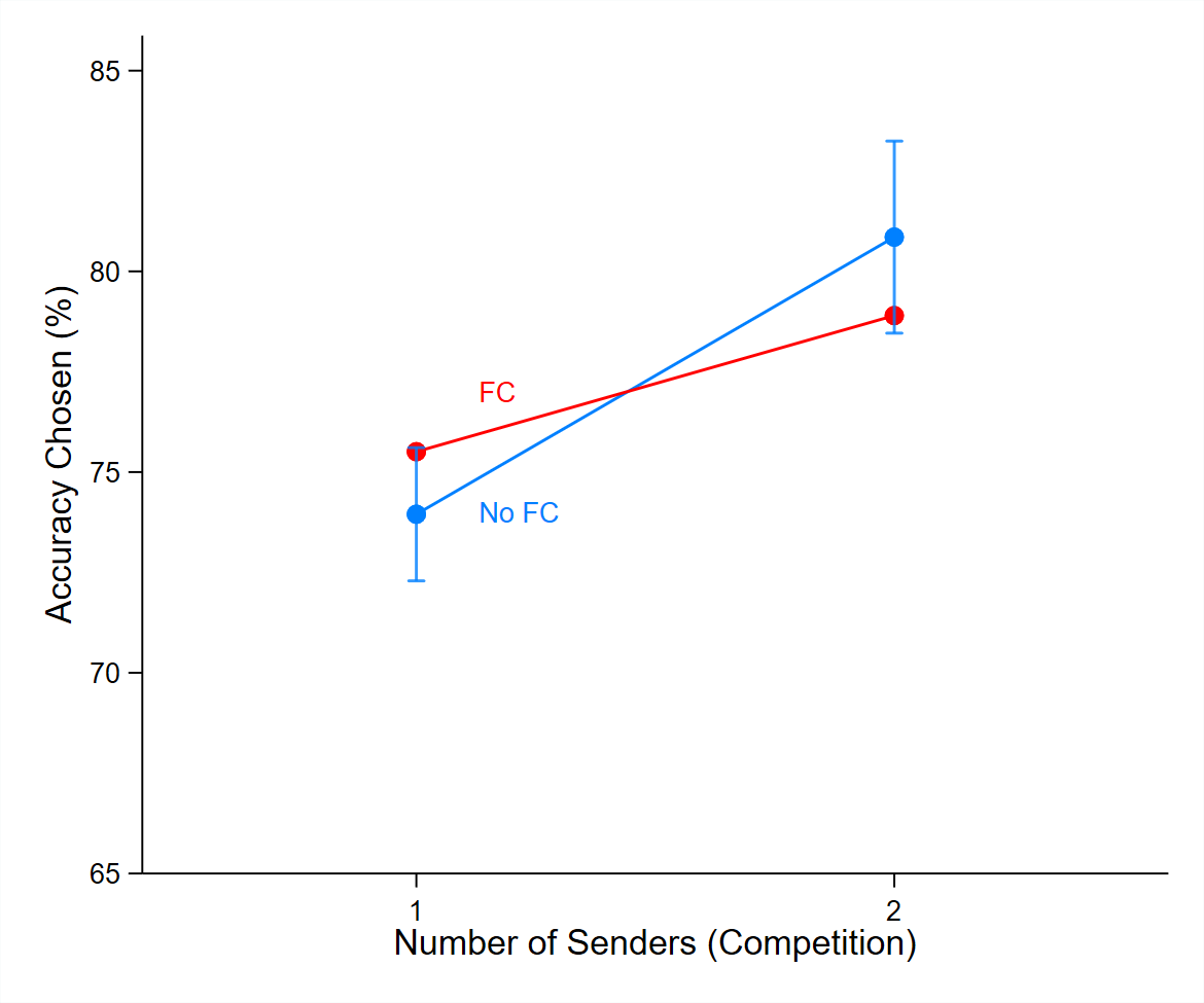
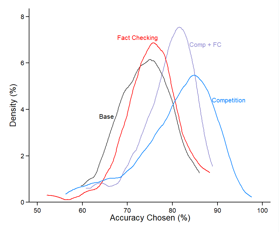
In the left panel, error bars are shown only for the base and competition treatments. These bars show that there is no statistically significant difference between the base and the fact-checking treatments, nor is there a statistically significant difference between the competition and the competition plus fact-checking treatments.

Treatment Effects on Receivers’ Choice

Unlike senders, receivers face a new decision in every interaction—because they are responding to an accuracy chosen by a different sender each time. For example, a receiver who sees an accuracy level of 50 percent in one round and 80 percent in the next round faces two entirely different decisions in each round. Therefore, we use the interaction-level data to calculate the average number of times receivers affirm for a given accuracy level. Specifically, we take averages at the interaction level to calculate $L(q)=\text{Pr}(a=1|q)$ , the likelihood of affirming for a given value of $q$ . Since messages with higher accuracy levels are more likely to get affirmed, we expect this function to be increasing in $q$ .⁹

Estimating this likelihood function using experimental data poses one problem in particular, which is that some accuracy levels were more popular among subjects than others. For example, accuracy levels of 54 percent and 56 percent were each chosen only once out of 2,340 accuracy choices made in the entire experiment. We resolve this issue by grouping accuracy choices into multiples of five, by rounding each accuracy to the nearest five. Hence, we use experimental data to estimate 11 points of the likelihood function, i.e., $L(q)$ for $q\in \{0.50, 0.55, 0.60, ...,1\}$ . Interestingly, subjects revealed a preference for choosing accuracy levels that are multiples of five (see figure 5 in Appendix B), making this approach almost a natural solution. Further, given that we are mostly interested in the general relationship between the probability of affirming and accuracy levels, and not the precise marginal effect of each accuracy level, we find this to be a very reasonable solution.

Figure 3 presents this likelihood function for the base treatment, the competition treatment, and the fact-checking treatment. To allow for easier comparison with the base treatment, we show the likelihood functions for the base and the competition treatments in the left panel and the likelihood functions for the base and the fact-checking treatments in the right panel. As expected, the likelihood function appears to be generally upward sloping in all three treatments. One notable observation in the base treatment is that the probability of affirming makes a significant jump between the accuracy levels of 65 and 70 percent. This suggests that many receivers use 70 percent as a threshold below which they are not willing to affirm. A sizable jump can also be observed between these values in the fact-checking treatment. For the competition treatment, however, we do not have sufficient data to check if receivers adopt a similar strategy because they almost always saw at least one message with an accuracy of at least 75 percent.

The left panel of figure 3 shows that for any given accuracy level, receivers in the competition treatment are less likely to affirm treatment than are receivers in the base treatment. This finding holds even if we control for whether the two messages seen by receivers in the competition treatment are different or the same. Given that subjects in the competition treatment are no more (nor less) risk averse than subjects in the base treatment (see table 5 in Appendix B), it must be something about merely seeing two messages, instead of one, that makes receivers more cautious (or risk averse) about affirming messages. This suggests that the mere presence of multiple news sources can cause people to question the veracity of the news even when both sources are saying the same thing.

In the fact-checking treatment, receivers are more likely to affirm a message than are receivers in the base treatment for accuracy levels of 60 percent or less. For accuracy levels greater than 60 percent, receivers in the fact-checking treatment are, in fact, less likely to affirm a message than receivers in the base treatment. However, except when the accuracy level is 70 percent, the likelihood of affirming is not significantly different (at the 5 percent level) between the two treatments. Therefore, we cannot conclude that fact-checking has an effect, one way or the other, on the likelihood of affirming a message.

Figure 3. Likelihood of Affirming

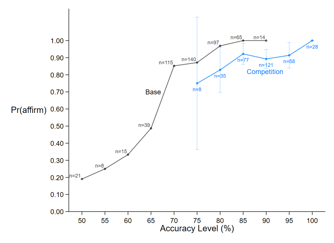
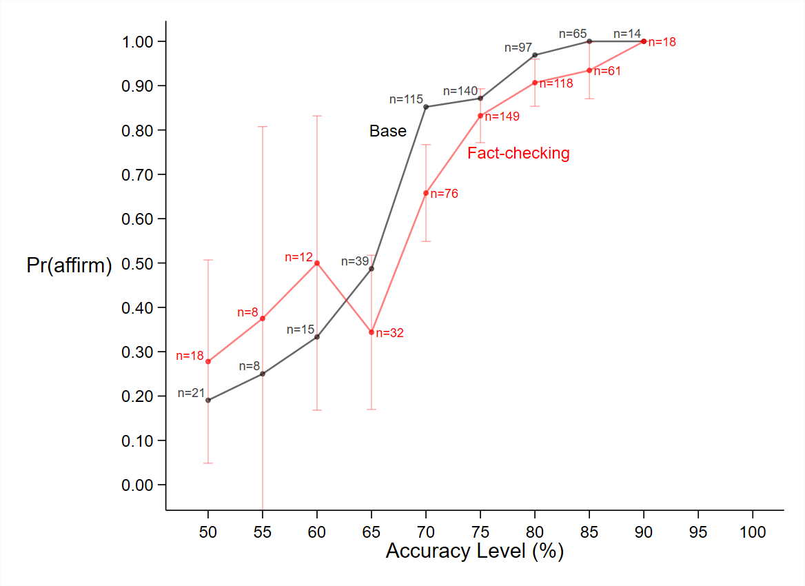
Notes: The vertical axis displays the proportion of times that receivers affirmed a message for the accuracy level given on the horizontal axis. The label $n$ denotes the number of interactions in which the corresponding accuracy level was chosen. Error bars show 95 percent confidence intervals. Accuracy choices that were made in 6 or fewer interactions (i.e., $n\leq6$ ) were omitted due to their high standard errors. For example, in the base treatment, an accuracy level of 85 percent was chosen in 65 (out of 540) interactions, and the receiver affirmed the message in 100 percent of these interactions. In the competition treatment, the higher accuracy level was 85 percent in 77 (out of 340) interactions, and receivers affirmed the message in 92 percent (71) of these interactions. This 8 percentage point difference between the base and the competition treatments is statistically significant (Mann-Whitney $p=0.0219$ ).

One possible explanation for fact-checking being ineffective is that there is only a one-in-four chance of a message getting randomly selected for fact-checking, and subjects may find this chance too low to be meaningful. If this is the reason, then increasing the chance of getting fact-checked should result in stronger effects from the fact-checking treatment. Assuming that those results would be in the same direction (just with greater magnitude and statistical significance), our result at least provides an insight about what would happen if fact-checking occurred with a greater probability. For media firms that do not make significant investments toward news accuracy (specifically choosing $q\leq 0.60$ ), the presence of a fact-checking process makes their news more believable. However, for media firms that invest more toward accuracy, fact-checking actually makes their news less believable than it would be without a fact-checking process.

Last, we try to determine how effective each policy intervention is toward reducing the amount of misinformation shared on social media. Given that our experimental decision of affirming a message represents the decision of sharing an article on social media, we can answer this question by looking at the number of false messages that get affirmed in each experimental treatment. Figure 4 shows the treatment effects on the proportion of false messages among the set of messages that were affirmed. In the base treatment, there were 428 (out of 520) interactions in which receivers affirmed a message. Out of these 428 affirmed messages, 106 (25 percent) were false. This means that under the conditions assumed in the base environment, about one in four news articles shared on social media would amount to misinformation. The media competition and the fact-checking interventions, when implemented alone, would each reduce this amount by about 6 to 7 percentage points, from 25 percent to about 18–19 percent. The effect of the competition plus fact-checking treatment is also statistically significant when compared to the base treatment but not when compared to the competition treatment or the fact-checking treatment.

Figure 4. Proportion of Affirmed Messages That Were Also False

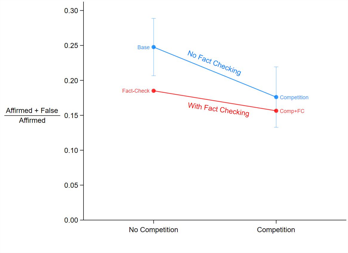
Notes: Error bars represent 95 percent confidence intervals and are shown for the base and the competition treatments. This graph provides some evidence of interaction between the two interventions: each intervention has a greater marginal effect when it is the only one present than when it is combined with the other.

Discussion

The goal of this study is to evaluate the effect of two policies of tackling misinformation, namely media competition and third-party fact-checking. Specifically, we see the effect of each policy on (i) how much money media firms invest toward their news accuracy, (ii) the willingness of consumers to share articles on social media, and (iii) the proportion of false news articles that ultimately make their way to social media. Our base treatment provides baseline values of each dependent variable that is used for comparison with other treatments.

Our main finding is that media competition has a significant effect on all three variables mentioned above. First, competition incentivizes media firms to devote more resources to news accuracy. Second, exposure to multiple news sources increases consumers’ standards of accuracy, causing them to become more selective about which articles to share on social media. Third, media competition lowers the proportion of false news articles shared on social media by approximately 7 percentage points.

One explanation for why the competition treatment has a stronger effect than the fact-checking treatment is that the former involves a greater degree of intervention. Specifically, the competition treatment doubles the number of media firms, while the fact-checking treatment only increases the probability of fact-checking by 25 percent. To test if this is indeed the case, an extension of this work may check the effect of fact-checking when it occurs with a greater probability (say, 50 percent) or the effect of a smaller increase in competition (say, from two to three firms).

Moreover, the simplistic assumption of our theoretical model provides an excellent starting point and ample room for adding various types of real-world complexities. Thus, it can serve as a valuable guide for future work in this area. For example, our model assumes that media firms only care about viewership and do not have a preference with regards to the message that gets shared on social media. In reality, this is not the case. Future studies can incorporate media firms’ preferences more accurately by giving senders in the experiment an additional reward if their favorite message gets shared on social media. Another example is that our model assumes that consumers only care about sharing the truth. A future study could make this model more realistic by allowing consumers to have a preference for sharing a particular message even if that message is the less accurate one.

Supplementary Appendix

Proofs and Examples

Proof of Proposition 1. (i) If the receiver affirms, his expected utility is $\mathbb{E}U_R= q v(1) + (1-q)v(0)=v(1)q$ . Since $v(1)$ is a constant, this is a monotonically increasing and one-to-one function of $q$ . If the receiver does not affirm, his utility is $U_R=v(0.5)$ , a constant. Thus, the receiver is indifferent between affirming and not affirming when $v(1)q=v(0.5) \Rightarrow q = \frac{v(0.5)}{v(1)}$ . We label this value as $q^B$ . Moreover, $q^B$ is unique because $y(q)=v(1)q$ and $y(q)=v(0.5)$ are two straight lines with different slopes and therefore can intersect at only one point.

(ii) The receiver’s complete strategy needs to specify what action he would take for any given value of $q$ . The receiver is indifferent between affirming and not affirming when $q=q^B=\frac{v(0.5)}{v(1)}$ . It is easy to see that for any $q>q^B$ , the receiver’s utility from affirming is strictly greater than his utility from not affirming, while for $q<q^B$, the receiver’s utility from affirming is strictly less than his utility from not affirming. We assume that the receiver resolves his indifference by affirming. Thus, his optimal strategy is

$a = \begin{cases} 1 &\text{if } q\geq q^B \\ 0 &\text{if } q < q^B \end{cases}$

.

Proof of Proposition 2. Given the receiver’s optimal strategy, for any $\widetilde{q}<q^B$ , the sender’s utility is $U_S(\widetilde{q}) = 0.5-c(q^B)\leq 0.5$ . Since $q^B<1$ , $c(q^B)<0.5$ , and $U_S(q^B)=1-c(q^B) >0.5$ . Therefore, $q^B$ strictly dominates $\widetilde{q}$ for all $\widetilde{q} < q^B$ . Since $c^\prime (q)>0$ , for any $\widetilde{q}>q^B$ , $c(\widetilde{q})>c(q^B)$ , and $U_S(\widetilde{q})<U_S(q^B)$ . Therefore, $q^B$ strictly dominates $\widetilde{q}$ for all $\widetilde{q} > q^B$ . Together, this shows that $q^B$ is the sender’s strictly dominant strategy.

Proof of Proposition 3. Case 1: $q_1 \neq q_2$ . Without loss of generality, suppose $q_1 > q_2$ . Then $v(1)q_1> v(1)q_2 \Rightarrow U_R(a=1)> U_R(a=2)$ . Thus, $a=2$ is strictly dominated by $a=1$ . There are two further subcases: (i) if $q_1\geq q^B$ , then by Proposition 1, the receiver’s optimal strategy is $a=1$ ; and (ii) if $q_1< q^B$ , then by Proposition 1, the receiver’s optimal strategy is $a=0$ .

Case 2: $q_1 = q_2$ . If $q_1=q_2<q^B$ , then both $a=1$ and $a=2$ are strictly dominated by $a=0$ . If $q_1=q_2\geq q^B$ , then the receiver has two optimal strategies: $a=1$ and $a=2$, as both of them result in the same expected utility.

Proof of Proposition 4. Taking the receiver’s strategy as given, this game can be reduced to a two-player game between two senders in which sender $i\in\{1,2\}$ needs to choose an accuracy of $q_i\in[0.5,1]$ .

We first show that there is no Nash equilibrium in pure strategies. If sender $i\in\{1,2\}$ plays $q_i=1$ , then sender $j$ ‘s best response is to play $q_j=0.5$ . However, this cannot be an equilibrium because sender $i$ has an incentive to unilaterally deviate to $q_i = 0.5+\varepsilon$ . Similarly, $q_i \in [0.5,1)$ also cannot be a Nash equilibrium because sender $j$ ‘s best response to that would be $q_j=q_i+\varepsilon$ , to which sender $i$ ‘s best response would be $q_i = q_j + \varepsilon$ . Therefore, there is no pure strategy Nash equilibrium for any $q_i \in [0.5,1]$ , which is the entire strategy space.

Next, we check if there is a Nash equilibrium in mixed strategies. Since each sender’s action space is continuous, we characterize a mixed strategy Nash equilibrium by specifying $F_i(q)$ , sender $i$ ‘s c.d.f., and its support, $[\underline{q_i},\overline{q_i}]$ . Moreover, Proposition 8 of Vartiainen (2007) shows that $F_i$ will contain an atom at $q_i=0.5$ (since this is an undominated strategy) and will be continuous over the support $(\underline{q_i},1]$ . All that is left now is to derive the functional form of $F_i$ and the lower bound of the support, $\underline{q_i}$ .

A necessary condition of a mixed strategy Nash equilibrium is that players must be indifferent between playing the equilibrium mixed strategy and playing any other undominated strategy. We can use this condition to derive the functional form of $F_i$ . In this case, this means that sender $i$ ‘s expected utility from playing the equilibrium mixed strategy should equal $U_{S_i}(q_i=0.5)=0.5$ . Thus, sender $i$ ‘s expected utility under a mixed strategy equilibrium would be

$\begin{align*} \text{Pr}(q_i \geq q_j)[1-c(q_i)] + [1-\text{Pr}(q_i \geq q_j)][0.5-c(q_i)] &= 0.5 \\ F_j(q_i) [1-c(q_i)] + [1-F_j(q_i)] [0.5-c(q_i)] &= 0.5 \\ F_j(q_i) &= 2c(q_i). \end{align*}$

Thus, the functional form of the c.d.f. is $F_i(q)=2c(q)$ .

Next, we find the lower-support $\underline{q_i}$ . We begin by stating that the area under the p.d.f. of the distribution over the support must equal 1. That is,

$F_i(1)=\int^1_{\underline{q}} f_i(q)dq=1$

$\begin{align*} &\Rightarrow \left[ 2c(q) \right]^1_{\underline{q}}=1 \\ &\Rightarrow 2c(1) - 2c(\underline{q})=1 \\ &\Rightarrow 1 - 2c(\underline{q})=1 \\ &\Rightarrow c(\underline{q})=0 \\ &\Rightarrow \underline{q}=0.5. \end{align*}$

Thus, the support of $F_i$ is the entire strategy space $[0.5,1]$ . However, since receivers never affirm a message whose accuracy is less than $q^B$ , all $q_i\in (0.5,q^B)$ are strictly dominated by $q_i=0.5$ and will be played with zero probability. Therefore, the support of $F_i$ will be $[q^B,1]$ plus an atom at $0.5$ .

Example 1. Suppose that $c(q)=2(q-0.5)^2$ and $v(x)=\sqrt{x}$ . What would be the SPNE of the game presented in the base environment?

The receiver would be indifferent between affirming and not affirming when $v(1)q = v(0.5) \Rightarrow q^B = \sqrt{0.5}$ . Thus, the receiver’s optimal strategy is to affirm whenever $q\geq \sqrt{0.5}$ (Proposition 1) and the sender’s optimal strategy would be to choose an accuracy of $q=\sqrt{0.5}=0.707$ (Proposition 2). The SPNE would be $\{q=\sqrt{0.5}; a=1\}$ .

Example 2. Suppose that $c(q)=2(q-0.5)^2$ and $v(x)=\sqrt{x}$ . What would be the SPNE of the game presented in the competition environment?

The receiver’s threshold for affirming is $q^B=\sqrt{0.5}$ (see example 1). Without loss of generality, let $q_i \geq q_j$ . If $q_i \geq \sqrt{0.5}$ , the receiver’s optimal strategy is to affirm $m_i$ . Otherwise, the receiver’s optimal strategy is to affirm neither of the two messages.

Based on Proposition 4, each sender will play a mixed strategy, assigning probabilities according to the c.d.f. $F(q) =4(q - 0.5)^2$ over the support $[\sqrt{0.5},1 ]$ .
Let $q^C$ denote the expected value of accuracy chosen by senders in the competition environment. In this example, this value evaluates to $q^C= \int_{q^B}^1 qf(q)dq = 0.724$ , which is slightly greater than $q^B=0.707$ . Thus, the competition environment encourages senders to invest only a little more money toward accuracy.

Additional Results

Summary Statistics

Tables 3 and 4 present summary statistics of subject-level variables. Table 3 shows key choice variables and demographic information, while table 4 shows subjects’ social preferences. The variable Accuracy Chosen represents the average of each subject’s average accuracy chosen in rounds in which the subject played as a sender. The variable Affirming Rate is the average of the proportion of times that each subject affirmed a message when playing as a receiver. Other than these two choice variables, none of the variables are significantly different across treatments, confirming the random assignment of subjects into treatments and suggesting that any differences in choice variables are only caused by differences in the treatment design.

Table 3. Summary Statistics

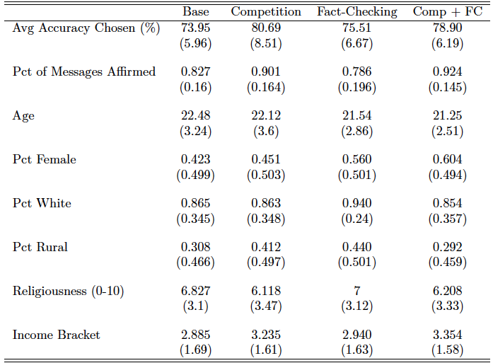
Notes: Parentheses show standard deviations. The variable Age indicates each subject’s age in years. The variables Pct Female, Pct White, and Pct Rural are binary variables indicating, respectively, whether the subject was female, was white, and grew up in a rural town. The variable \textit{Religiousness} is a self-reported measure of how religious a person is, on a scale from 0 to 10. The variable \textit{Income Bracket} is categorical and ranges from 0 to 5, with 0 = <$30,000; 1 = $30,000–$50,000; 2 = $50,000–75,000; 3 = $75,000–$100,000; 4 = $100,000–$150,000; and 5 = $\geq$ $150,000.

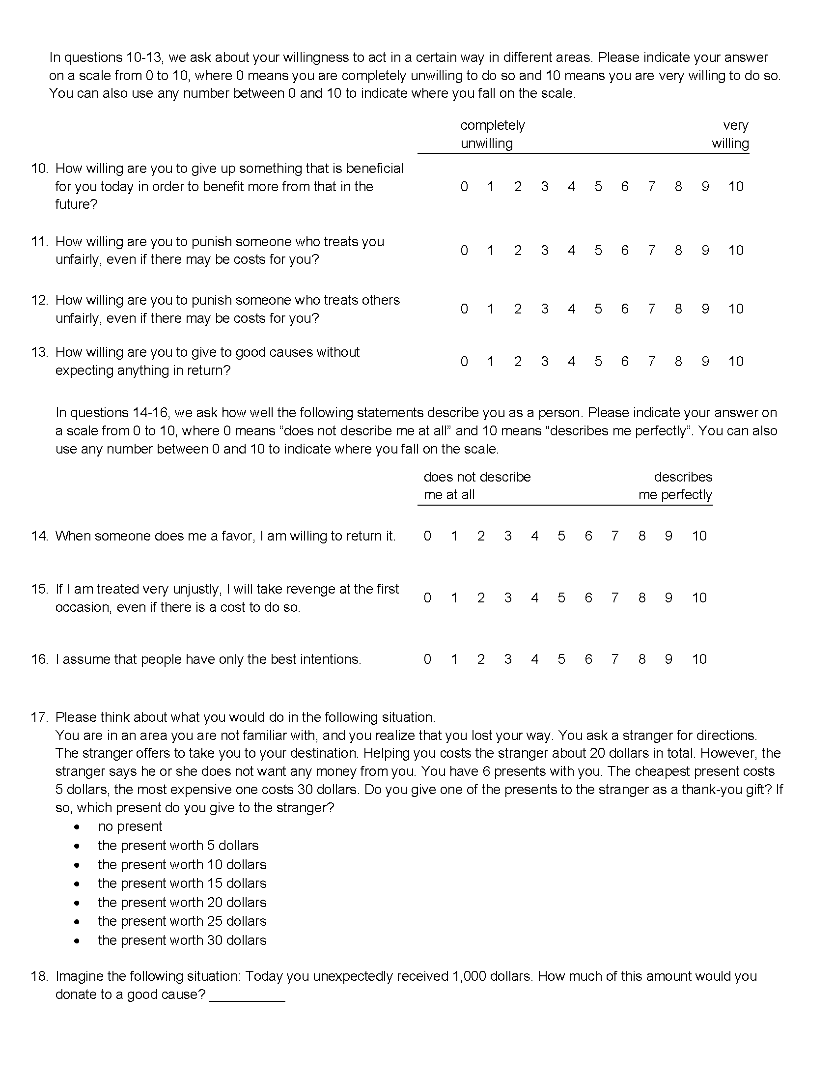
We use responses from the social preferences questions (questions 9–18 of the post-experiment questionnaire) to construct six social preferences variables, namely Risk Taking, Patience, Altruism, Trust, Positive Reciprocity, and Negative Reciprocity. We follow the method presented by Falk et al. (2018, p. 1,653, table 1). Specifically, we first standardize subjects’ responses to questions 9–18 along with their decisions in the bomb task. Then, to create the Risk Taking variable, we combine question 9 with the bomb task, giving each of these a weight of 0.5. To create the Altruism variable, we take the weighted average of questions 13 and 18 using weights of 0.365 and 0.635, respectively. Negative Reciprocity is a weighted average of question 11 (with a weight of 0.313), question 12 (with a weight of 0.313), and question 15 (with a weight of 0.374). Positive Reciprocity is a weighted average of question 14 (with weight 0.485) and question 17 (with weight 0.515). The variables Patience and Trust are simply standardized versions of questions 10 and 16, respectively. These standardized social preferences variables are presented in table 5.

Table 4. Summary Statistics for Social Preferences Variables

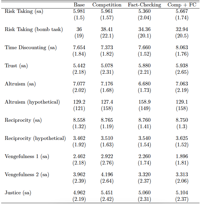
Notes: Parentheses show standard deviations. Variables suffixed by (sa) are subjects’ self-assessments on a scale from 0 to 10. The variable Risk Taking (bomb task) represents the number of boxes collected by subjects in the incentivized bomb task. Variables suffixed by (hypothetical) are based on subjects’ responses about how they would behave in certain hypothetical scenarios. The actual questions that were used to elicit these preferences are presented along with the experiment instructions (see figure 12 in Appendix C).

Table 5. Social Preferences, Combined and Standardized

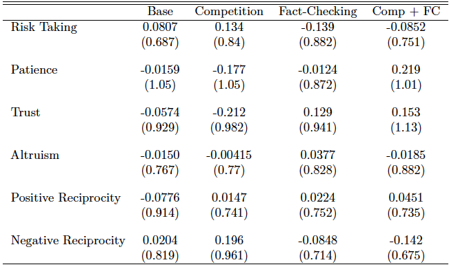
Notes: Parentheses show standard deviations. Means within each treatment are not zero because these variables were not standardized at the treatment level but for the entire data.

Regression Results

Table 6 presents OLS regression results with Accuracy Chosen as the dependent variable. The first regression only includes indicator variables for treatments as independent variables. Therefore, the regression coefficients represent treatment effects relative to the base treatment. The results show that none of the demographic variables nor social preferences variables—not even Risk Aversion—have any significant correlation with senders’ accuracy choice. In fact, these results tell us nothing more than what we already know from figure 2, which is that the competition treatment has the strongest effect on senders’ accuracy choices.

Table 6. Regression Results
(Dependent Variable: Sender’s Accuracy Choice)

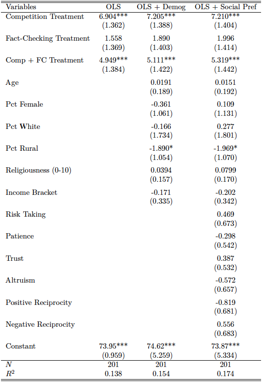
Notes: Parentheses show standard errors. ***p < 0.01, **p < 0.05, *p < 0.1

Figure 5. Histogram of Accuracy Levels Chosen by Senders

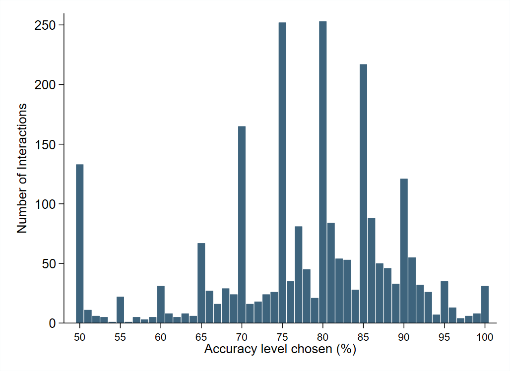
This histogram contains 2,340 accuracy choices made by senders (note there are more senders than interactions because some interactions had two senders). For some reason, accuracy levels that were multiples of five were more popular than their neighbors.

Experiment Instructions

Figures 6–10 show the experiment instructions and decision-making screens that were seen by subjects in the base treatment. Instructions for other treatments are omitted to avoid redundancy but can be provided by the authors upon request. Figures 11 and 12 show the post-experiment questionnaire. Questions 1–8 of the questionnaire collect some basic demographic information, whereas questions 9–18 elicit subjects’ social preferences using selected questions from the Global Preferences Survey (Falk et al., 2018).

Power Analysis

We started with two pilot sessions, one for the base treatment and the other for the competition treatment. We found that the average accuracy chosen by senders in the base treatment was 73.9 percent (sd= 5.74, N=16) and in the competition treatment was 83.7 percent (sd=7.66, N=18). This meant that as few as 9 subjects in each of the two treatments would give us a power of 80 percent. Nonetheless, we decided, as part of our pre-analysis plan, to recruit approximately 50 subjects per treatment for two reasons. First, we did not know if the effect size in the other treatments (namely fact-checking and competition plus fact-checking) relative to the base treatment would be as large as that of the competition treatment. Second, our current resources allowed us to recruit up to 200 subjects comfortably, but further recruitment would require more resources.

We ended up recruiting 201 subjects and found a that competition had a large effect on accuracy choice while fact-checking had only a marginal effect. Specifically, the effect size of the competition treatment had a power of 99.7 percent, while the effect size of the fact-checking treatment had a power of only 23.3 percent. For the competition plus fact-checking treatment, we got a power of 98.1 percent.

Figure 6. Screenshot of Experiment Instructions

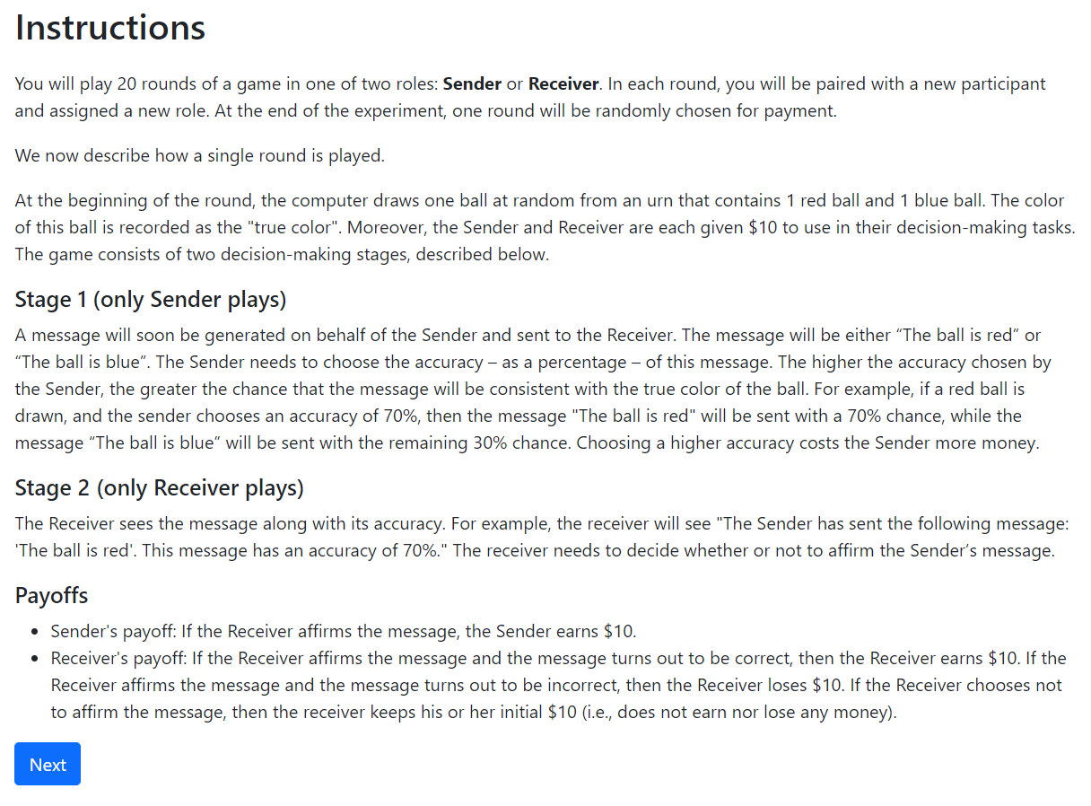
Figure 7. Screenshot of Sender’s Decision

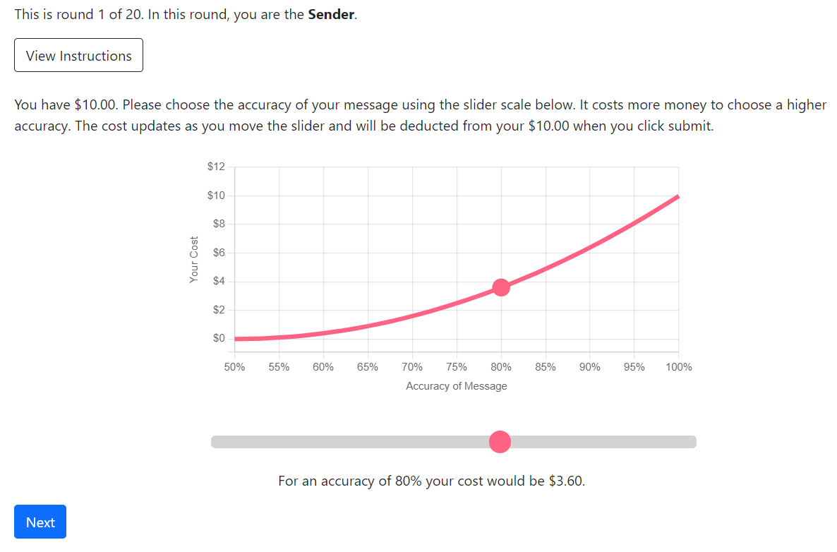
We use an interactive graph to explain that the cost function is convex (which helps us avoid using mathematical language or equations). As subjects move the pink dot on the slider scale, the numbers below the slider scale and the point on the graph both update in real time.

The following box pops up upon clicking the “View Instructions” button in the screenshot above.

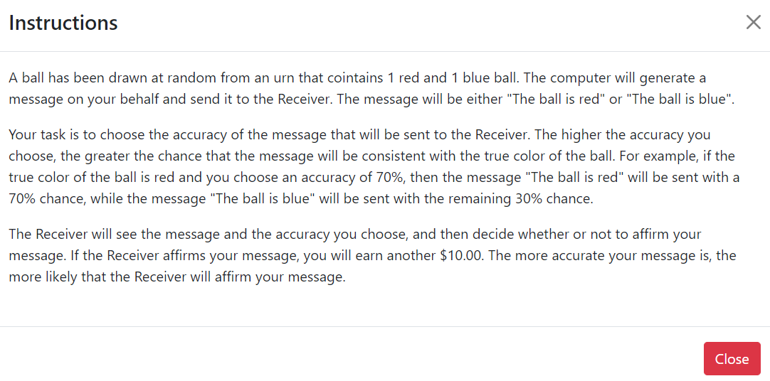
Figure 8. Screenshot of Receiver’s Decision

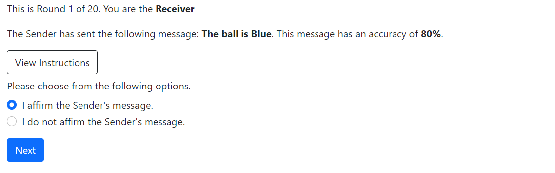
The following box pops up upon clicking the “View Instructions” button in the screenshot above.

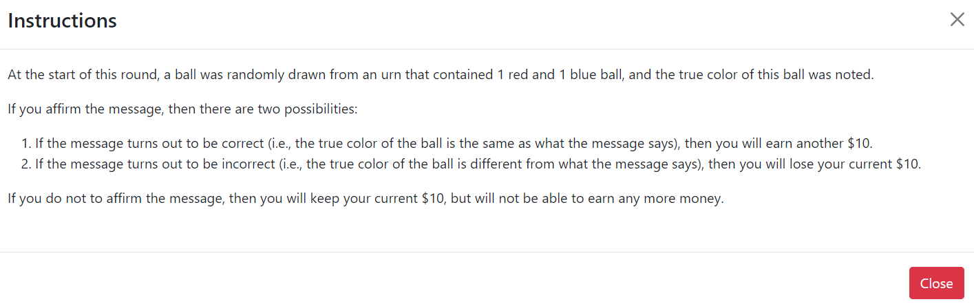
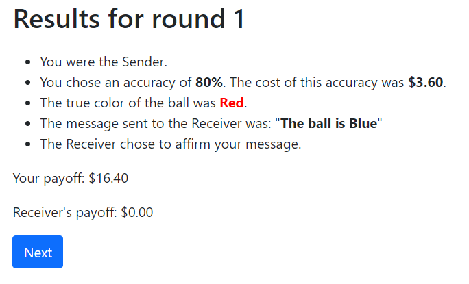
Figure 9. Screenshot of Results (Shown at the End of Each Round)

(a) Sender’s Results

(b) Receiver’s Results

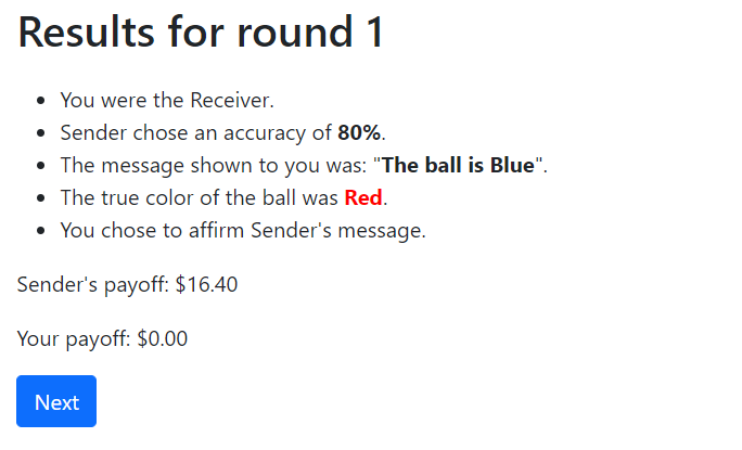
Figure 10. Random Selection of Round for Payment

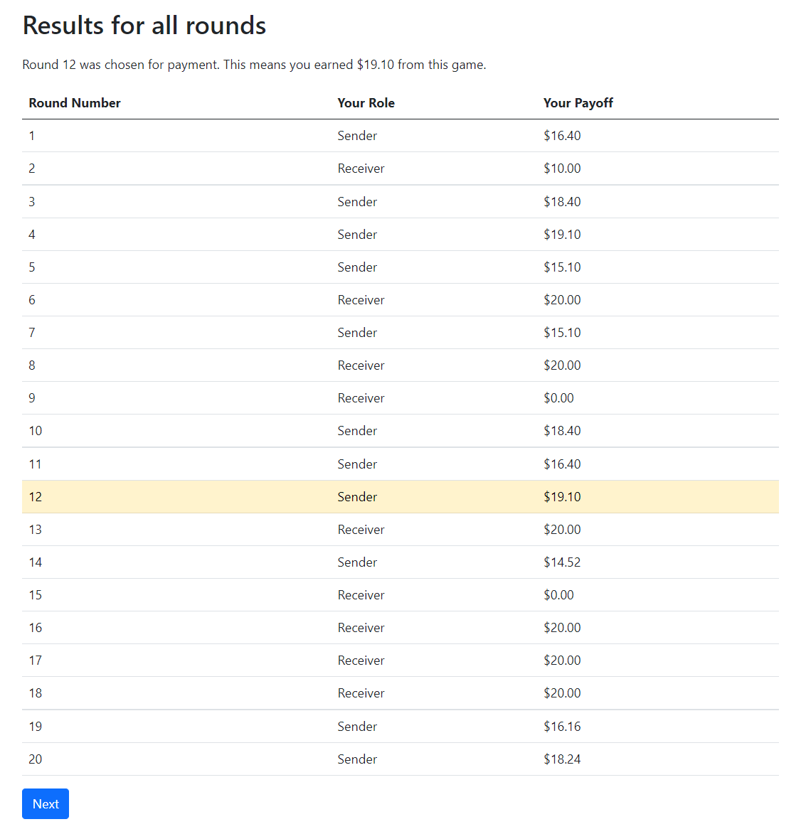
Figure 11. Questions 1–9 of the Post-Experiment Questionnaire

Figure 12. Questions 10–18 of the Post-Experiment Questionnaire

References

Allen, J., A. A. Arechar, G. Pennycook, and D. G. Rand (2021). Scaling up fact-checking using the wisdom of crowds. Science Advances 7 (36), eabf4393.

Baye, M. R., D. Kovenock, and C. G. De Vries (1993). Rigging the lobbying process: An application of the all-pay auction. The American Economic Review 83 (1), 289–294.

Blasco, A. and F. Sobbrio (2012). Competition and commercial media bias. Telecommunications Policy 36 (5), 434–447.

Charness, G., U. Gneezy, and A. Imas (2013). Experimental methods: Eliciting risk preferences. Journal of Economic Behavior & Organization 87, 43–51.

Chen, D. L., M. Schonger, and C. Wickens (2016). otree—an open-source platform for laboratory, online, and field experiments. Journal of Behavioral and Experimental Finance 9, 88–97.

Crosetto, P. and A. Filippin (2013). The bomb risk elicitation task. Journal of Risk and Uncertainty 47 (1), 31–65.

Falk, A., A. Becker, T. Dohmen, B. Enke, D. Huffman, and U. Sunde (2018, 05). Global evidence on economic preferences. The Quarterly Journal of Economics 133 (4), 1645–1692.

Gentzkow, M. and J. M. Shapiro (2008). Competition and truth in the market for news. Journal of Economic perspectives 22 (2), 133–154.

Graves, L. (2016). Deciding What’s True: The Rise of Political Fact-Checking in American Journalism. Columbia University Press.

Jahanbakhsh, F., A. X. Zhang, A. J. Berinsky, G. Pennycook, D. G. Rand, and D. R. Karger (2021). Exploring lightweight interventions at posting time to reduce the sharing of misinformation on social media. Proceedings of the ACM on Human-Computer Interaction 5 (CSCW1), 1–42.

Kriplean, T., C. Bonnar, A. Borning, B. Kinney, and B. Gill (2014). Integrating on-demand fact-checking with public dialogue. In Proceedings of the 17th ACM Conference on Computer Supported Cooperative Work & Social Computing, pp. 1188–1199.

Lazer, D. M., M. A. Baum, Y. Benkler, A. J. Berinsky, K. M. Greenhill, F. Menczer, M. J. Metzger, B. Nyhan, G. Pennycook, D. Rothschild, et al. (2018). The science of fake news. Science 359 (6380), 1094–1096.

Lejuez, C. W., J. P. Read, C. W. Kahler, J. B. Richards, S. E. Ramsey, G. L. Stuart, D. R. Strong, and A. Brown (2002). Evaluation of a behavioral measure of risk taking: The balloon analogue risk task (BART). Journal of Experimental Psychology: Applied 8 (2), 75.

Mullainathan, S. and A. Shleifer (2005). The market for news. American Economic Review 95 (4), 1031–1053.

Pennycook, G., A. Bear, E. T. Collins, and D. G. Rand (2020). The implied truth effect: Attaching warnings to a subset of fake news headlines increases perceived accuracy of headlines without warnings. Management Science 66 (11), 4944–4957.

Pennycook, G., Z. Epstein, M. Mosleh, A. A. Arechar, D. Eckles, and D. G. Rand (2021). Shifting attention to accuracy can reduce misinformation online. Nature 592 (7855), 590–595.

Shearer, E. (2021). More than eight in ten Americans get news from digital devices. Pew Research Center.

Tacchini, E., G. Ballarin, M. L. Della Vedova, S. Moret, and L. De Alfaro (2017). Some like it hoax: Automated fake news detection in social networks. Technical Report UCSC-SOE-17-05, School of Engineering, University of California, Santa Cruz.

Vartiainen, H. (2007). Comparing complete information all–pay auctions. Unpublished manuscript.

Wang, W. Y. (2017, July). “liar, liar pants on fire”: A new benchmark dataset for fake news detection. In Proceedings of the 55th Annual Meeting of the Association for Computational Linguistics (Volume 2: Short Papers), Vancouver, Canada, pp. 422–426. Association for Computational Linguistics.

Yaqub, W., O. Kakhidze, M. L. Brockman, N. Memon, and S. Patil (2020). Effects of credibility indicators on social media news sharing intent. In Proceedings of the 2020 CHI Conference on Human Factors in Computing Systems, pp. 1–14.

Reducing Misinformation on Social Media: An Experimental Evaluation of Two Policy Interventions

Executive Summary

Resources

Focuses

Introduction

Model

Base Environment

Setup

Equilibrium

Competition Environment

Setup

Equilibrium

Fact-Checking Environment

Setup

Equilibrium

Competition and Fact-Checking Environment

Setup

Equilibrium

Summary of Results and Testable Hypotheses

Experiment Design

Experimental Procedures

Description of Treatments

Base Treatment

Competition Treatment

Fact-Checking Treatment

Competition Plus Fact-Checking Treatment

Results

Data

Treatment Effects on Senders’ Choice

Treatment Effects on Receivers’ Choice

Discussion

Supplementary Appendix

Proofs and Examples

Additional Results

Summary Statistics

Regression Results

Experiment Instructions

Power Analysis

References

Executive Summary

Resources

Related Publications

Related News

Related Blogs

Focuses

Introduction

Model

Base Environment

Setup

Equilibrium

Competition Environment

Setup

Equilibrium

Fact-Checking Environment

Setup

Equilibrium

Competition and Fact-Checking Environment

Setup

Equilibrium

Summary of Results and Testable Hypotheses

Experiment Design

Experimental Procedures

Description of Treatments

Base Treatment

Competition Treatment

Fact-Checking Treatment

Competition Plus Fact-Checking Treatment

Results

Data

Treatment Effects on Senders’ Choice

Treatment Effects on Receivers’ Choice

Discussion

Supplementary Appendix

Proofs and Examples

Additional Results

Summary Statistics

Regression Results

Experiment Instructions

Power Analysis

References