Parched Power Plants: The Role of Markets and Technology in Power Plants’ Drought Responses

Hutchens, Andrew; Edwards, Eric; Fell, Harrison; Kern, Jordan

1 Introduction

Climate change continues to have wide-ranging effects on the environment and society, often affecting how the two interact. Most policies have addressed climate change through decarbonization efforts in high-emission sectors such as transportation and electricity, particularly as extreme weather events have increased in frequency and stressed the electricity grid (US EPA, 2023a; Tyran, 2023). The electricity sector is especially vulnerable to climatic shocks that climate change can amplify,¹ particularly drought. This is because thermoelectric power plants (which still produce the majority of electricity in the United States, around 60 percent in 2021 (US EIA, 2022)) rely on water for their cooling systems.² In effect, droughts diminish water quantity and quality, thereby decreasing plants’ efficiency and increasing their marginal cost of generation (Putman and Harpster, 2000; Lakovic et al., 2010; Pattanayak, Padhi, and Kodamasingh, 2019).

Competitive (or deregulated) wholesale power markets should efficiently reallocate generation and provide incentives for plants to adapt to drought’s exogenous efficiency and cost shocks. However, does this happen in practice? That is, do power plants located in competitive wholesale power markets experience generation reallocation and adapt to drought as competitive theory predicts? Do plants that are instead located in areas serviced by vertically integrated monopoly utilities, where no competition exists, respond oppositely by bearing the efficiency loss and marginal cost increase? And how do plants’ responses to their own drought state vary with the extent of drought in their operating area? In this paper, we leverage the heterogeneity in electricity market structure across the contiguous United States and exogenous drought shocks to estimate the effect of drought on plant-level efficiency and generation in different markets and market-level drought conditions.³^,⁴

We contribute to the literature within the energy-water nexus in ways that highlight the close relationship between energy and water resources. First, we use high-resolution satellite-derived data on the PDSI⁵ that enables us to obtain plant-level measures of drought conditions over time. These data allow us to construct more precise estimates of local or plant-level drought conditions than coarser measures (e.g., climate-region-level PDSI) used in prior work (e.g., Eyer and Wichman, 2018). Second, we shed light on the efficacy of competitive electricity markets for achieving cost-minimizing generation reallocation across thermoelectric power plants. Such insight is key for informing the management of remaining thermoelectric plants during the decarbonization of the electricity sector.

Third, we provide the first evidence of plant-level efficiency responses to drought using two-way fixed effects regression models. Efficiency adjustments have been shown to be a viable mechanism for responding to cost shocks such as fuel price changes (Doyle and Fell, 2018) and even water temperature changes (Henry and Pratson, 2016), which are a symptom of drought. This evidence augments previous work analyzing plant-level generation responses to drought (Eyer and Wichman, 2018; Mamkhezri and Torell, 2022; Qiu et al., 2023). Finally, we extend previous research’s analyses of plant responses by allowing them to vary based on the extent of drought in a plant’s market (market-drought). This allows us to estimate drought’s effects on plant responses through two avenues: a plant’s own-drought state (which affects their own efficiency and marginal cost) and market-drought (which affects a plant’s responses by altering the market-level electricity supply curve, potentially changing the incentives a plant faces).⁶

Our results broadly show that wholesale electricity markets work as intended for reallocating generation from water-intensive to less water-intensive plants during drought (i.e., shifting generation toward less water-intensive and lower-cost natural-gas-fired plants). For capacity factor (a measure of plant usage), combined-cycle natural-gas-fired market plants experience increased capacity factor during drought as their market allocates more generation to them. However, we also find some regions’ nonmarket plants experiencing the same capacity factor effects as their market counterparts, indicating that nonmarket entities find mimicking market outcomes to be advantageous. We also find that the capacity factor of market coal-fired plants decreases during drought, albeit only in Texas during drought-intensive years, lending some credence to the importance of drought persistence and frequency. For heat rate (a measure of plant efficiency), we chiefly find that only market peaker plants using simple-cycle steam generators decrease their heat rate (improve their efficiency) during drought as expected.

Our analyses of market-drought’s effects mostly find that market plants experience higher capacity factors when they are not in drought but more of their market is. Conversely, they experience lower capacity factors when they are in drought and less of their market is affected by it. However, we find very little evidence of market-drought affecting market plants’ heat rate. The capacity factor effects are in line with our theoretical expectations for market-drought that are based on wholesale electricity markets’ use of a merit order to construct a supply curve that orders plant offers from least to greatest cost. When a market plant is not in drought but more of their market is, the plant will be called upon to generate more often since their costs are not increased by drought, unlike the rest of the market. Conversely, when a market plant is in drought and less of their market is, then less of the market’s supply curve is reordered due to increased costs while the plant is shifted out. This shift reduces the generation that the plant is called upon to provide.

Shedding light on plant-level efficiency and generation responses to drought is important for better understanding the role of markets in the water-energy nexus amid decarbonization efforts and a growth in reliability concerns as extreme weather events occur more frequently. The transition to a decarbonized energy sector will not happen overnight, so society must contend with the existing fleet of fossil fuel plants and its adaptation to climate change until renewable energy sources comprise most of the generation fleet. The crux of this paper is the difference in adaptation incentives and responses across market types (i.e., between competitive markets and vertically integrated monopolies), whether such a difference ultimately brings about favorable changes in plant operations, and how the extent of drought in a market affects its salience. Plants operating in market (deregulated) areas face incentives to remain cost-competitive and mitigate or fully offset drought’s effects on their marginal cost through efficiency improvements⁷ or market-enacted changes to their generation, while plants operating in nonmarket (regulated) areas are cogs in their respective utility’s monopoly machine and face no such incentives. By virtue of being regulated, utilities operating plants in nonmarket areas are not allowed to earn profit on maintenance or fuel costs, which both affect plant efficiency; these are operating expenses that utilities are not allowed to mark up (Kibbey, 2021).⁸ These plants (and the utilities that operate them) then have little to no market incentives to improve their efficiency or change their generation. Thus, large swaths of the United States have their electricity needs serviced by entities that may be relatively unresponsive to climate change’s effects.⁹ As for competitive markets, it remains to be empirically verified if competitive incentives actually work as intended in the context of climate-change-induced cost/efficiency shocks such as drought.¹⁰ If competitive markets work as intended, then they could be a viable method of shifting electricity generation toward less costly plants and incentivizing improved plant efficiency, enabling emissions reductions and cost savings in the face of climate change.

Previous work has largely focused on either the market-level effects of drought on generation, capacity, or electricity prices (van Vliet, Vögele, and Rübbelke, 2013; McDermott and Nilsen, 2014; Pechan and Eisenack, 2014; Kern and Characklis, 2017; Byers et al., 2020; Fonseca et al., 2021) or on the firm-level effects of drought on financial outcomes or investment behavior (Kern and Characklis, 2017; Bogmans, Dijkema, and van Vliet, 2017). Ganguli, Kumar, and Ganguly (2017) and Chandel, Pratson, and Jackson (2011) diverge from most of the literature by examining national-scale generation effects of drought and policy’s effects on power plant water usage, respectively. Moreover, many existing studies employ simulations rather than econometric models like the ones we use in this paper (van Vliet, Vögele, and Rübbelke, 2013; van Vliet et al., 2016). The papers that are most similar to ours are Eyer and Wichman (2018) and Golombek, Kittelsen, and Haddeland (2011). However, Eyer and Wichman focus only on generation effects using a coarser drought measure (climate-region-level PDSI), and Golombek, Kittelsen, and Haddeland use a simulated market-level model to identify efficiency effects. We use a much finer drought measure and provide plant-level analyses of efficiency and generation responses.

The rest of this paper proceeds as follows. Section 2 provides essential information on the relationship between thermoelectric power plants and drought and on US wholesale electricity markets. Section 3 elucidates our conceptual model of market versus nonmarket plant drought responses and theoretical model of plant efficiency and generation responses to market-drought from a competitive, profit-maximization perspective. Section 4 describes the data used for estimating our econometric models, which are detailed in Section 5. Section 6 reports the results of estimating our econometric models of plant responses. Section 7 discusses the results’ general and policy implications as well as avenues through which unanticipated results may have formed. Section 8 concludes.

2 Background and Industrial Setting

2.1 Thermoelectric Power Plant Water Usage and Drought

Thermoelectric power plants are plants that use steam turbine or combined-cycle generating units.¹¹ Such plants require water to cool their generators’ steam back into liquid form for reuse in their power generation process. Plants extract cooling water from surface waters (e.g., lakes, rivers, and streams) and feed it into a condenser, where used steam exiting the turbine enters and is cooled (condensed) back into liquid form. The extracted cooling water, having absorbed the steam’s heat, is then discharged directly back to its source (in once-through cooling systems) or to a cooling tower/pond (in recirculating cooling systems).¹² The cooled steam water is then pumped back to the boiler to be heated into steam again. The steam proceeds to turn the blades of the turbine and the rotor shaft of the generator before reentering the condenser to repeat the process all over again. Figure 1 provides a graphical illustration of thermoelectric plants’ water usage process (for those with once-through cooling systems).¹³ Note that the process entails differing levels and rates of water withdrawal and consumption¹⁴ across cooling system types, namely once-through, recirculating, dry, and hybrid.¹⁵

Figure 1. Basic Illustration of How Water Is Used at Thermoelectric Power Plants

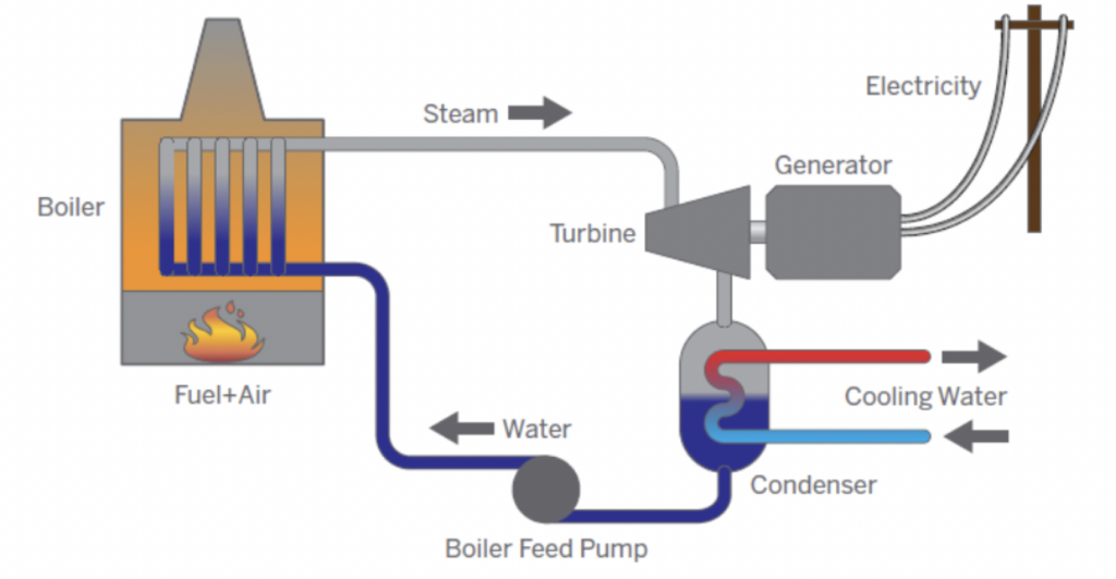
Notes: Figure source is Reimers (2018)

Drought is generally defined to be precipitation deficiency over an extended time period (e.g., a month). The American Meteorological Society goes a step further and defines it as “a period of abnormally dry weather sufficiently long enough to cause a serious hydrological imbalance” (Drought.gov, n.d.). For the purposes of this paper, we focus specifically on hydrological drought as it is most salient to power plant operations.¹⁶ Hydrological drought is prolonged precipitation deficiency in surface (e.g., lakes, rivers, and streams) or subsurface (e.g., groundwater) water supply (National Drought Mitigation Center, 2022). That is, it concerns the lack of water in the hydrological system that manifests in the form of unusually low river streamflow and unusually low levels of water in other surface waters and groundwater (Van Loon, 2015).

Low streamflows are a direct consequence of drought, and high water temperatures are a symptom that typically accompanies drought (Kimmell and Veil, 2009). Thermoelectric power plants are generally vulnerable to low streamflows, high ambient air temperatures, and high water temperatures (Bartos and Chester, 2015).¹⁷ Thus, regardless of a generating unit’s prime mover or a plant’s cooling system, drought essentially imparts two effects upon plants: an increase in the marginal cost of generation and a decrease in generating capacity (or derating). The marginal cost effect is our main channel of interest, and it results from drought increasing intake water temperature or decreasing available water levels.

Previous research has established that both higher intake water temperatures and lower streamflow negatively affect plants’ generating capacity (van Vliet et al., 2012; Bartos and Chester, 2015) and efficiency (Stillwell, Clayton, and Webber, 2011; Zammit, 2012; Colman, 2013; Denooyer, 2015; McCall, MacKnick, and Hillman, 2016; Petrakopoulou, 2021). In this paper, we measure efficiency with a plant’s heat rate HR, defined as

$H R=\frac{\text { Fuel combusted (MMBtus) }}{\text { Electricity generated (MWhs) }}$

In short, lower efficiency (higher heat rate) results from higher condenser pressure; the engineering literature has shown that both higher intake water temperatures and lower streamflow increase condenser pressure (Putman and Harpster, 2000; Pattanayak, Padhi, and Kodamasingh, 2019). Higher pressure within a plant’s condenser (where steam is cooled back into liquid form) is associated with lower turbine efficiency for both single-cycle steam turbines and the steam engine component of combined-cycle turbines. This is because an increase in condenser pressure causes a turbine’s endpoint enthalpy to increase, leading to a loss in generation.

Higher steam flow is then needed to maintain the prior level of generation, and this higher steam flow is achieved by increasing the turbine’s throttle and combusting more fuel (Putman and Harpster, 2000; Lakovic et al., 2010; Pattanayak, Padhi, and Kodamasingh, 2019). This increased fuel combustion to produce the same amount of electricity is the source of lessened efficiency. Lakovic et al. (2010), Zammit (2012), Denooyer (2015), and Pattanayak, Padhi, and Kodamasingh (2019) all show that higher cooling water temperature leads to higher condenser pressure and lower efficiency. McCall, MacKnick, and Hillman (2016), Pattanayak, Padhi, and Kodamasingh (2019), and Petrakopoulou (2021) show that a lower cooling water flow rate or water availability increases condenser pressure and lowers efficiency overall. See Appendix A for a more detailed exposition of how drought affects condenser pressure and, ultimately, plant efficiency.

2.2 US Wholesale Electricity Markets

In this paper, we focus on markets for wholesale electricity generation (i.e., not retail markets that sell power to end users such as households) since these are the markets that power plants operate and face external cost shocks (e.g., drought). The United States is home to two types of wholesale electricity markets: competitive markets (located in deregulated regions) and vertically integrated monopolies (located in the regulated utilities’ service territories).

Figure 2 illustrates the spatial distribution of US wholesale electricity markets and how we classify market and nonmarket plants. We designate the seven regions governed by the seven RTOs and ISOs as our market areas since they operate competitive wholesale electricity markets. Consequently, we classify all plants operating in these RTOs/ISOs as market plants. These RTOs/ISOs are the California Independent System Operator (CAISO), Electric Reliability Council of Texas (ERCOT), Southwest Power Pool (SPP), Midcontinent Independent System Operator (MISO), PJM Interconnection (PJM), New York Independent System Operator (NYISO), and ISO New England (ISONE). We designate all of the
balancing authority areas in the gray areas as nonmarket areas, that is, areas serviced by a vertically integrated monopoly utility.¹⁸ We classify all plants operating in the gray areas as nonmarket plants¹⁹ and define two regions to allow for heterogeneous responses based on regional differences in utility operations:²⁰ West (which includes all balancing authorities in the Western Interconnection besides CAISO²¹^,²²) and Southeast (which is effectively captured by the SERC Reliability Corporation’s regional footprint).²³ The nonmarket balancing authority areas within these regions are serviced by a single vertically integrated monopolist utility that owns and operates generation, transmission, and distribution resources.

Figure 2. Map of US RTOs

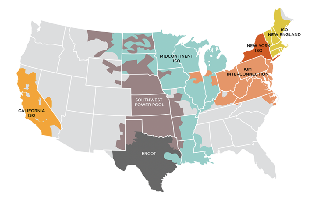
Notes: Figure source is Sustainable FERC Project (2020).

Our analyses are carried out in several configurations: full sample, Western Interconnection, Eastern Interconnection, Texas, and individual RTOs/ISOs (see Section 5 for details on these configurations). Some states in our nonmarket regions overlap with states that are part of our market areas or RTOs/ISOs, but we classify plants based on whether they are in an RTO/ISO or not even if they are located in a state that is partially part of an RTO/ISO and a nonmarket area. For example, CAISO includes the state of California, but California also contains some plants that are part of the Balancing Authority of Northern California (BANC). Plants that operate within CAISO are classified as market plants, and those that operate as part of BANC are classified as nonmarket plants.

Competitive wholesale electricity markets separate the market for electricity generation from electricity transmission and distribution. The demand side of these markets typically consists of electric utilities and nonutility power providers,²⁴ while the supply side consists of independent power producers and electric utilities. These markets generally operate as follows.²⁵ The RTO/ISO first determines how much electricity demand (or load) there is or will be to serve. Electricity suppliers submit bid prices (equal to their marginal cost of generation) for the amount of electricity that they choose to supply. The RTO/ISO then performs a process called economic dispatch to order suppliers (plants) by marginal cost (ascending from lowest cost to highest cost) and construct the electricity supply curve.

The final ordering is called the merit order. Moving down the merit order is equivalent to moving to the left in the ordering (and supply curve), while moving up is equivalent to moving to the right in the ordering (and supply curve). The result is a discontinuous step function for the electricity supply curve,²⁶ where the market-clearing price received by all suppliers is the marginal cost of the market-clearing or marginal supplier (i.e., the last supplier called upon to fulfill load).²⁷ Changes to marginal cost due to exogenous factors like drought naturally affect plants’ position on the supply curve and, consequently, whether they are inframarginal, marginal, or not called upon to generate at all. Increased marginal cost moves a plant up (or to the right) the merit order and supply curve, while decreased marginal cost moves a plant down (or to the left) the merit order and supply curve.

Operations in regulated or nonmarket areas serviced by vertically integrated monopoly utilities look much different than competitive wholesale markets. Like RTOs, these utilities also determine how much load to serve and operate economic dispatch of their plants. But that is where the similarities end. Utilities mainly serve load using their own plants according to their own decisions regarding plant dispatch, but they can also engage in bilateral electricity trading with other utilities.²⁸ The electricity prices faced by end users such as households are fixed by regulation that is typically performed by state utilities commissions; no wholesale electricity price arises because there is no competition in generation. By law, these utilities are guaranteed a predetermined rate of return on capital investments or expenses, but they are not allowed to earn any profit on operating expenses such as fuel or maintenance costs. This type of regulation incentivizes investment in infrastructure (e.g., new power lines, generators, and entire plants) over improving existing technologies or operations (e.g., improving efficiency or reducing maintenance costs) since the latter amounts to increasing operating expenses that utilities cannot earn profit on.

3 A Conceptual and Theoretical Framework for Power Plant Drought Responses

In this section, we motivate our empirical analyses with a conceptual and theoretical exposition of plant behavior in and out of drought. We first elucidate our conceptual framework for differing drought responses between market and nonmarket plants. This framework allows us to ground our econometric models in market structure theory and define our market versus nonmarket hypotheses. We then cast market plants’ drought responses as the solution of a competitive profit-maximization problem that introduces drought as an exogenous variable in plants’ marginal cost and hours in operation functions. This approach enables us to derive comparative statics and hypotheses that we test empirically using the data described in Section 4 and econometric framework detailed in Section 5.

As Section 3.3 describes in more detail, our profit-maximization model takes the perspective of a plant operating in a competitive wholesale market (i.e., a market plant), which implies that we expect nonmarket plants to respond differently or ambiguously (possibly due to unobserved private operating factors) or not respond at all to market-drought (i.e., that market-drought does not enter their objective function). Given the lack of competition in nonmarket regions, the most salient drought factor for nonmarket plants should be their own drought condition, hence our focus on the responses of market plants to market-drought.

Although market plants’ only choice variable in our theoretical model is their change in heat rate, our econometric framework tests drought’s effects on plants’ heat rate and capacity factor. This is because we assume that plants produce as much as they can whenever they are called upon to produce even if they are derated by drought. Any changes (reductions) in capacity factor are due to drought increasing marginal cost, which thereby affects whether a plant is inframarginal, marginal, or not called upon and, consequently, their capacity factor. Thus, our empirical results for capacity factor effects are a result of marginal cost changes and not necessarily plants choosing different generation levels.

Our conceptual and theoretical models assume that drought is sufficiently salient to plants so as to influence them to respond. Given climate change’s growing impacts on weather events, this seems like a reasonable assumption to make. However, it is possible that drought frequency and persistence affect whether or not plants respond to drought at all;²⁹ in the context of this paper, persistence refers to drought duration, and frequency refers to how often drought events occur (not necessarily consecutively). This is a possibility that we explore in our empirical analyses by studying plant responses during temporal subsets in which drought was frequent or persistent (by market area).

Finally, our theoretical model posits an undefined planning horizon for plant decisions. This allows us to derive comparative statics for situations where plants’ planning horizons coincide with drought frequency. However, it also reflects that we do not know what plants’ planning horizons are with respect to heat rate or capacity factor changes specifically in response to drought. Our empirical analyses implicitly assume a monthly planning horizon due to our monthly data on plant generation and heat rate, but it is possible that plants respond to drought according to longer or shorter periods.

3.1 Market versus Nonmarket Plants’ Own-Drought Responses

We define own-drought to be an individual plant’s drought condition (e.g., in drought; not in drought; mild, moderate, or severe drought). Drought reduces the quantity of water available (the quantity effect) and increases water temperature (the temperature or quality effect). Through these two effects, drought ultimately imparts the following effects upon plant operations:

reduced generating capacity (or derating), caused by drought’s quantity effect
increased marginal cost, caused by drought’s quantity and quality effect

We now briefly describe the pathways drought takes to impart these effects on capacity and marginal cost, beginning with capacity (specifically capacity factor):³⁰

Drought’s quantity effect causes the water level to decrease, diminishing the plant’s water supply.
Plants become capacity constrained (or derated); that is, their maximum output is reduced due to the decreased water supply.
Plants’ output is reduced below what it would have been absent drought conditions,³¹ decreasing capacity factor.

Keeping with drought’s quantity effect, we now turn our attention to marginal cost:

Drought’s quantity effect causes the water level to decrease, diminishing the plant’s water supply.
Water’s mass flow rate into condensers decreases (Petrakopoulou, 2021).
Heat rate increases (efficiency decreases).
Reduced efficiency increases the per unit of electricity expenditure on fuel³² such that more fuel is needed to produce the same amount of electricity → marginal cost increases.

Finally, marginal cost is also affected by drought’s quality effect:

Drought’s quality effect increases water temperature.
Plants’ intake water temperatures increase.
Heat rate increases (efficiency decreases).
Reduced efficiency increases the per unit of electricity expenditure on fuel such that more fuel is needed to produce the same amount of electricity → marginal cost increases.

These capacity factor and marginal cost effects would manifest if plants did not respond to drought at all (i.e., if they did not adjust their efficiency or if their capacity factor was not changed by supply curve changes due to drought). In reality, market plants face private and market incentives to adjust their efficiency and will likely experience changes to their capacity factor based on realized drought conditions. On the other hand, nonmarket plants do not face such market incentives to remain cost-competitive and instead have the option of passing on increased costs due to drought to consumers. In addition, their operating utilities/entities do not have access to a centralized wholesale electricity market and instead must rely on bilateral trading with other utilities/entities. Thus, we expect differing drought responses between market and nonmarket plants.

With respect to capacity factor effects, because drought increases plants’ marginal cost of generation, market areas should reallocate generation from water-intensive plants (that experience the greatest cost increases due to drought) to less water-intensive plants (that experience smaller cost increases than water-intensive plants) to meet demand at least cost. In terms of electricity supply in market areas, this means that plants whose cost increases are shifted right on the supply curve (or merit order), with water-intensive plants being shifted farther to the right than less water-intensive ones. Coal and natural gas are the primary fossil fuels used in thermoelectric plants, and because coal-fired plants use more water than natural-gas-fired plants (Union of Concerned Scientists, 2013; US EIA, 2023a), we classify coal plants as water intensive and natural gas plants as less water intensive.³³ Even if both gas- and coal-fired plants are in drought, gas-fired plants should experience higher capacity factor as generation is reallocated to them instead of coal-fired plants despite the costs of both plant types increasing. The key here is that gas-fired plants’ costs increased by less than coal-fired plants’ cost increase due to drought. Thus, we expect market plants’ capacity factor to increase in drought if they are natural gas fired and to decrease in drought if they are coal fired.

Nonmarkets do not face the same competitive cost-minimization incentives as market plants, and they must rely on costlier bilateral trading instead of a centralized wholesale market. Therefore, we do not expect the same reallocation from coal to natural gas to occur among nonmarket plants, and instead expect drought to decrease capacity factor for all plant types (through derating). However, there are two scenarios in which nonmarket plants may behave like market plants. First, nonmarket operating entities or utilities may exercise fleet-wide generation reoptimization when drought occurs.³⁴ This behavior would make sense if the reliability benefits of generation reoptimization are large enough. Second, some nonmarket regions may have sufficient access to low-cost bilateral trading to closely mimic wholesale markets.

Heat rate effects in market versus nonmarket plants are more straightforward. Drought should cause heat rate decreases in market plants since they face competitive incentives to reduce their marginal cost and remain cost-competitive during drought. Conversely, nonmarket plants face no such incentives and are also not allowed to earn a return on operating expenses (like improving efficiency by reducing heat rate). Instead, they may prefer to make new capital investments (on which they can earn a regulated return) as opposed to reducing their marginal cost through efficiency improvements that they are not allowed to mark up. Therefore, we expect drought to cause heat rate increases in nonmarket plants as they bear the efficiency loss due to drought.

Our overarching market versus nonmarket hypothesis is therefore the following:

H0: Drought increases capacity factor for natural-gas-fired market plants, decreases capacity factor for coal-fired market plants and all nonmarket plants, causes market plants to decrease their heat rate, and causes nonmarket plants to experience increased heat rate.

3.2 Market Plants’ Market-Drought Responses: Mechanisms and Intuition

The own-drought effects (on heat rate and capacity factor) described in Section 3.1 likely depend on the drought condition of the market that they operate in (i.e., market-drought; the extent of drought in a market that we define as the proportion of total thermoelectric capacity that is in drought at some time period).³⁵ Own-drought shifts a plant’s position in its market’s merit order (through its effects on plant marginal cost), and market-drought affects the extent of that shift by affecting the overall change in the market’s merit order or supply curve.³⁶ Thus, for any individual plant $i$ , three principal cases arise:

Case 1: All plants in its market are in drought (i.e., a high proportion of the market’s total capacity is in drought; market-drought is equal to one), including plant $i$ .
Thus, all plants experience an increase in marginal cost, the entire supply curve shifts up, and the merit order remains unchanged. No plant has an incentive to change their efficiency, and they are called upon to generate with the same probability as without drought (since the entire supply curve is shifted up). Therefore we expect $i$ ’s capacity factor to be unchanged or decrease slightly and heat rate to increase (efficiency to decrease).
Case 2: Plant $i$ is in drought, but very few other plants in its market are in drought (i.e., a low proportion of the market’s total capacity is in drought; market-drought is low).
Plant $i$ experiences an increase in marginal cost and gets shifted up the merit order and supply curve. This increase in marginal cost and consequent higher position on the supply curve cause $i$ to generate less (since it is less likely to be inframarginal) and reduce its heat rate to remain cost-competitive. The plant may also be derated due to drought, which would also reduce its generation by reducing its capacity. Thus, we expect $i$ ’s capacity factor to decrease and heat rate to decrease (efficiency to increase) or be unchanged.
Case 3: Plant $i$ is not in drought, but many other plants in its market are (i.e., a high proportion of the market’s total capacity is in drought; market-drought is high).
Plant $i$ ’s marginal cost does not increase, but other plants’ marginal costs do, so they move up on the merit order and supply curve. Consequently, plant $i$ is more likely to be inframarginal, and so its generation (capacity factor) would increase. This case has ambiguous effects on $i$ ’s heat rate (drought is not exogenously lowering it, but there are external benefits to further lowering marginal cost, so heat rate may be unchanged or minimally decreased).

Intermediate cases are easily captured by varying own or market-drought.³⁷ For example, one can travel closer toward case 1 from case 2 by increasing the proportion of a market’s total capacity that is in drought (i.e., increasing market-drought). Moreover, one can switch between case 2 and case 3 by reducing/increasing own-drought.

Finally, note that although the pathways connecting drought to capacity and generation still apply to plants in nonmarket areas, these nonmarket plants do not abide by the logic in the three previous principal cases. This is because such plants are all owned and operated by a single monopoly utility, facing no competition from other plants in their utility’s service area. Thus, only own-drought conditions should be relevant for nonmarket plants’ efficiency and generation responses to drought.

3.3 A Model of Market Plant Profit-Maximization with Drought

We now generalize the plant behavior described in Section 3.2 and explore drought’s effects on plant capacity factor and efficiency using a model of plant-level profit-maximization. Because plants operating in nonmarket areas do not face the competitive incentives discussed in Section 3.2 (by virtue of functioning in a monopoly), we specifically model the profitmaximization performed by competitive plants operating in market areas. The implication of this choice and Section 2.2’s description of vertically integrated monopoly utilities is that nonmarket plants either ambiguously or do not adjust their own-drought responses based on market-drought. This may be due to unobserved operational factors that drive their private decisions or to market-drought not entering their profit-maximizing objectives.

Suppose that in each month, a plant operating in a competitive wholesale electricity market chooses its change in heat rate over a month $\Delta H R$ to maximize its per-month profits. The choice variable follows Doyle and Fell (2018) and is given by $\Delta H R=H R_0-H R_1$ , where $H R_0$ is a plant’s heat rate before any changes and $H R_1$ is its chosen (possibly changed) heat rate at the end of a month. With this definition, the choice of a lower heat rate (an efficiency improvement) is represented by choosing $\Delta H R>0$ . Plants can adjust their heat rate in several ways and not only when exogenous shocks like drought occur. Examples of heat rate adjustments include improving steam trap management, improving feedwater chain system performance, improving the maintenance of generators’ air filtration units, enhancing or upgrading unit components,³⁸ and better managing controllable parameters like boiler flue gas oxygen content.³⁹^,⁴⁰ These adjustments are costly,⁴¹ so a rational profit-maximizing firm would only perform such adjustments when the benefits of doing so outweigh the costs.⁴² Moreover, the frequency and consistency of drought may affect whether or not a plant actually adjusts its efficiency at all. It is possible that plants do not respond to infrequent or short-lived drought. While our theoretical model implicitly assumes that drought is sufficiently salient to plants, we test whether plants’ responses depend on drought frequency or consistency in our empirical analyses.

Let own-drought and market-drought be denoted by $D_o$ and $D_m$ , respectively, such that higher values of either correspond to worse drought. Finally, let $f$ denote the per-unit price of fuel. Because drought’s ultimate effect (absent a response by the plant) is an increase in marginal cost, let marginal cost of generation MC be given by

$M C=M C\left(f, D_o, \Delta H R\right),$

with partials $\frac{\partial M C}{\partial f}>0$ , $\frac{\partial M C}{\partial D_o}>0$ , and $\frac{\partial M C}{\partial \Delta H R} \leq 0$ .⁴³ To clarify the plant’s decision-making process in adapting its heat rate (efficiency) to drought, below is the sequence of events faced by all market plants:

Exogenously determined drought states are realized (e.g., no drought, mild drought, severe drought).
Plants observe $D_o$ , $D_m$ , load conditions in their balancing authority area, and how
much their own capacity and heat rate is affected (i.e., $H R_0$ ).
Plants choose their change in heat rate $\delta H R$ given their observed (and now fixed) $H R_0$ .

We model the intuition and generalization of the principal cases in Section 3.2 by exploiting the fact that drought affects plants’ position on the supply curve through its effects on $MC$ . This amounts to drought affecting plants’ ability to be an inframarginal or marginal generator and the total number of hours in a month in which a plant has positive generation (either as an inframarginal or marginal generator).⁴⁴ A plant’s number of hours in a month with positive generation depends on its own-drought and market-drought. Let the number of hours in a month in which a plant has positive generation be given by

$H=H\left(f, D_o, D_m, \Delta H R\right),$

with partials $\frac{\partial H}{\partial f} \leq 0, \frac{\partial H}{\partial D_o} \leq 0, \frac{\partial H}{\partial D_m} \geq 0, \frac{\partial H}{\partial \Delta H R} \geq 0$ .⁴⁵These partials state that an increase in own-drought (worsened own-drought) or fuel price decreases the number of hours in which a plant has positive generation; an increase in market-drought (worsened market-drought) increases the number of hours in which a plant has positive generation; and improving efficiency increases the number of hours in which a plant has positive generation.

Letting the cost of heat rate changes be given by $C(\Delta H R)$ (with $C^{\prime}(\cdot)>0$ ) and the
per-unit market price of electricity be $p$ , the plant’s profit-maximization problem is

(1) $\begin{equation*}\underset{\Delta HR}{\text{max}}\;\;\; \pi=\left[p-MC\left(f,D_o,\Delta HR\right)\right]qH\left(f,D_o,D_m,\Delta HR\right)-C\left(\Delta HR\right),\end{equation*}$

with first-order condition (omitting functional arguments for brevity)

(2) $\begin{equation*}\displaystyle\frac{\partial\pi}{\partial \Delta HR}=(p-MC)q\frac{\partial H}{\partial\Delta HR}-qH\frac{\partial MC}{\partial\Delta HR}-\frac{dC}{d\Delta HR}=0.\end{equation*}$

Differentiating Equation (2) with respect to $D_m$ yields

(3) $\begin{equation*}\frac{\partial^2\pi}{\partial\Delta HR\partial D_m}=(p-MC)q\frac{\partial^2 H}{\partial\Delta HR \partial D_m}-q\frac{\partial MC}{\partial\Delta HR}\frac{\partial H}{\partial D_m}.\end{equation*}$

Assuming that $\displaystyle\frac{\partial^2 H}{\partial\Delta HR \partial D_m}\geq 0$ ,⁴⁶ we can sign Equation (3)’s cross-partial: $\displaystyle\frac{\partial^2\pi}{\partial\Delta HR\partial D_m}\geq 0$ , which tells us that efficiency must increase (i.e., $\Delta HR$ must increase and heat rate must decrease) when market-drought increases. However, this result and the assumption made to obtain it are only true for a plant that is not in drought. If a plant is in drought and market-drought $D_m$ increases (more capacity/plants in the market are in drought), then increasing efficiency (or $\Delta HR$ ) would have a smaller positive effect on $H$ since more of the supply curve remains relatively unchanged. In this case, $\displaystyle\frac{\partial^2 H}{\partial\Delta HR \partial D_m}\leq 0$ , meaning that Equation (3) now has an ambiguous sign. Given this dichotomy in Equation (3)’s sign, we form the following hypotheses:

H1: Plants that are not in drought will improve their efficiency (decrease their heat rate) and experience an increase in capacity factor (due to marginal cost advantages from market-drought and/or their own efficiency) as market-drought increases.
H2: Plants that are in drought will improve their efficiency (decrease their heat rate) and experience a decrease in capacity factor as market-drought decreases.

We can explore the effect of own-drought on plants’ $\Delta HR$ choice by differentiating Equation (2) with respect to $D_o$ , which yields

(4) $\begin{equation*}\frac{\partial^2\pi}{\partial\Delta HR \partial D_o}=(p-MC)q\frac{\partial^2 H}{\partial\Delta HR \partial D_o}-q\frac{\partial MC}{\partial D_o}\frac{\partial H}{\partial\Delta HR}-qH\frac{\partial^2 MC}{\partial\Delta HR \partial D_o}-q\frac{\partial H}{\partial D_o}\frac{\partial MC}{\partial\Delta HR}.\end{equation*}$

Even with assumptions on the signs of the cross-partials in Equation (4), the equation still has an ambiguous sign. We attribute this ambiguity to our approach to modeling plants’ drought responses, particularly the dependence between plants’ own-drought reaction and market-drought summarized in Section 3.2’s three principal cases: how a plant’s profit-maximizing choice of efficiency ( $\deltaH R$ ) depends on its own-drought $D_o$ depends on market-drought $D_m$ . Given this theoretical bulwark, we formulate the following hypothesis:

H3: Plants in drought have varying market-drought responses based on the severity of their own-drought condition.

4 Data

Our empirical tests of Section 3’s Hypotheses H0–H3 use monthly⁴⁷ mover-fuel-level data (hereafter referred to as PMFT for prime mover (PM) and fuel type (FT), respectively), where “mover” refers to prime mover (i.e., the generating technology, such as steam (ST) or combined-cycle (CC)) and fuel is either natural gas (NG) or coal (CO).⁴⁸ All of our data are publicly available and span January 2010 through December 2020. Because only steam-powered generating units require cooling water, our final analysis is restricted to plants that use steam or combined-cycle generators. Moreover, for plants that use multiple steam-powered units with different coal types, we aggregate each unit’s data into one steam-powered coal-fired (ST-CO) observation. For example, if plant Z has a steam-powered bituminous coal-fired unit and a steam-powered refined coal-fired unit, our data combine both units’ data into one ST-CO entity observed over time. We apply a similar aggregation process to combined-cycle plants insofar as we combine the separate data on the gas and steam turbines into one CC-NG entity observed over time.

Our main electricity data sources are the EIA’s Form EIA-923 and Form EIA-860. We obtain PMFT-level generation in MWh, fuel consumption in MMBtu, prime mover type, and fuel type from Form EIA-923. We obtain plant location (i.e., city, county, zip, state, and coordinates), plant sector, plant balancing authority area, and generator-level nameplate capacity from Form EIA-860. Plant-level nameplate capacity is calculated by summing the nameplate capacity of all generators at a plant. For plants with multiple generators of the same PMFT combination, we also create PMFT-level nameplate capacity by summing the nameplate capacity of generators with the same PMFT combination. Total renewable generation in each balancing authority area is calculated using data from the EIA’s Form EIA-923 by summing the generation of all renewable plants within each area in each month. Finally, we obtain monthly Henry Hub natural gas prices from the EIA’s natural gas data page.

Our measure of plant-level generation is capacity factor, which is our first dependent variable.⁴⁹^,⁵⁰ This choice allows us to account for differing plant sizes/capacities. We divide generation by monthly nameplate capacity in each month to construct PMFT-level capacity factor. Our measure of efficiency is plant-level heat rate, which is our second dependent variable. We divide fuel consumption by generation in each month to construct heat rate in MMBtu/MWh. In addition, we drop all observations with outlier (and potentially erroneous) values for heat rate, specifically dropping all observations with a heat rate greater than 100 MMBtu/MWh.⁵¹^,⁵²

We obtain data on our demand-side control variables from the US Federal Energy Regulatory Commission’s (FERC) Form 714. This source provides monthly load and net interchange in MWh at the balancing authority area level. Load is a measure of total monthly electricity demand in each month, allowing us to explicitly control for electricity demand. The net interchange variable is essentially a measure of net imports/exports. It enables us to control for transmission heterogeneity across balancing authority areas that may permit some areas to better respond to drought via greater electricity imports from other areas.

Our measure of drought is the PDSI. The PDSI uses precipitation and temperature data to estimate relative dryness using a physical water balance model, which enables it to account for climate change’s effects on drought (National Center for Atmospheric Research, 2022). The index ranges from –10 to 10, where values below –1 indicate drought conditions and decreases in the PDSI constitute decreases in water supply. We use a novel data set named gridMET from the Climatology Lab at the University of California Merced that provides daily PDSI measurements at a 4km or 1/24th degree grid cell resolution for the contiguous United States from 1979 to present.⁵³^,⁵⁴

Figure 3. Snapshot of gridMET Data, February 2010

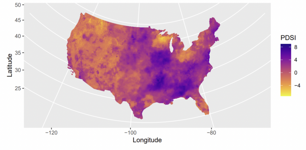
gridMET’s high spatial resolution enables us to construct a nearly plant-level measure of drought conditions using PDSI data from the grid cells closest to each plant.⁵⁵ For each plant in our sample, we identify the 10 nearest 4km grid cell centroids to the plant and calculate the inverse-distance-weighted (IDW) average PDSI across the 10 PDSI values. That is, for plant $p$ in month-year $t$ with nearest grid cells $g_i=1,\dots,10$ each possessing raw PDSI values $RP_{g_it}$ , we construct their IDW PDSI $PDSI_{it}$ using

(5) $\begin{equation*}PDSI_{it}=\displaystyle\sum_{g_i=1}^{10}\omega_{g_{i}} RP_{g_it},\end{equation*}$

with the normalized weights $\omega_{g_i}$ calculated using $\omega_{g_i}=\displaystyle\frac{u_{g_i}}{\sum_{g_i=1}^{10}u_{g_i}}$ , where $u_{g_i}=\displaystyle\frac{1}{d(l_i,l_{g_i})}$ and $d(l_i,l_{g_i})$ is the geodetic distance between plant $i$ and grid cell $g_i$ ‘s centroid.

Using EIA 860’s data on generator nameplate capacity and the gridMET PDSI data, we calculate each (market or nonmarket) area’s market-drought, defined as the proportion of capacity in drought in each month.⁵⁶^,⁵⁷ This variable is calculated in each month as the amount of capacity in drought (calculated by summing the capacities of all plants in drought, that is, with $PDSI_{it}\leq -1$ , in a given month) divided by the total capacity (calculated by summing the capacity of all plants in a given month). We construct this variable for both total capacity (i.e., across all PMFTs) and for the following key PMFTs: natural-gas-fired steam generation (ST-NG), natural-gas-fired combined-cycle generation (CC-NG), and coal-fired steam generation (ST-CO).

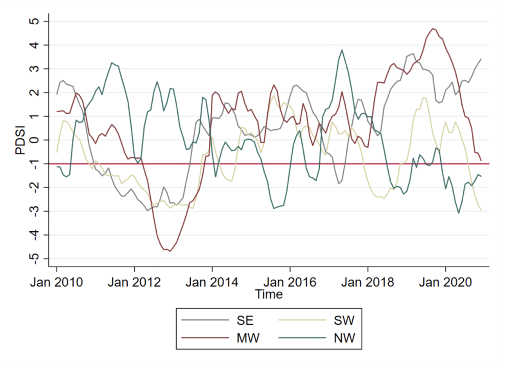
Figure 4. Mean Monthly PDSI by Market Area

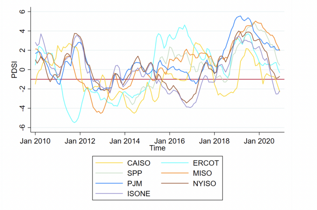
Notes: Averaged over all plants in each area. Recall that PDSI≤ −1 constitutes being in drought.

Figure 5. Mean Monthly PDSI by Nonmarket Region

Notes: Averaged over all plants in each region. Recall that PDSI≤ −1 constitutes being in drought.

5 Econometric Framework

Our econometric analyses test our plant-level efficiency and capacity factor response hypotheses from Section 3 through several approaches. We begin by testing our market versus nonmarket area Hypothesis H0 using a binary own-drought indicator (Section 5.1). We then shed more light on H0 by using a categorical own-drought variable representing no-drought, mild drought, moderate drought, and severe drought conditions instead of a binary own-drought indicator (Section 5.1). Next, we test our market-drought Hypotheses H1 and H2 by estimating the effect of market-drought interacted with a binary own-drought indicator on market plants (Section 5.2.1).

Finally, we allow own-drought to vary in severity to test H3 by estimating the effect of market-drought interacted with a categorical own-drought variable representing no-drought, mild drought, moderate drought, and severe drought conditions (Section 5.2.2). We estimate each approach across all generation technologies that are susceptible to drought (i.e., all technologies that use a steam or combined-cycle prime mover, namely ST or CC prime mover plants) and also broken out by key PMFTs (prime mover PM and fuel type FT combinations) to allow responses to differ by technology (since operating cost and intrinsic efficiency differ across technologies).⁵⁸

We use two-way fixed effects regression models in all of our approaches. To clearly compare outcomes between drought and nondrought conditions, and to partially allow for nonlinear own-drought effects,⁵⁹ we use a binary own-drought indicator and a categorical set of own-drought bins.⁶⁰ These binary and binned approaches also capture discrete changes that are potentially more salient to plants than finer-scale changes in water supply that would be captured by continuous PDSI. The PDSI bins are constructed in order of worsening severity as detailed in Table 3.⁶¹

We allow for heterogeneous responses by area by estimating all of our models separately for each US grid interconnection and RTO/ISO.⁶²^,⁶³ Moreover, in all of our specifications, we control for unobserved time-invariant plant-level characteristics (e.g., age, management style, and technology brand) through PMFT fixed effects. We control for unobserved entity-invariant factors that affect all plants in a region in the same manner and change over time (e.g., seasonal plant maintenance schedules, climatological fluctuations, government policies, and input costs)⁶⁴ using month-by-year-by-interconnection fixed effects.

5.1 Own-Drought’s Effects on Market versus Nonmarket Plants

To test whether drought’s effects vary between market and nonmarket plants according to H0, we first use a binary drought indicator interacted with a binary market plant indicator. We omit the no-drought bin $D_0$ in our estimating equations to estimate drought’s effects on nonmarket and market plants relative to the no-drought case (i.e., no drought $D_0$ is our reference drought category). Our estimating equations then take the following forms:

(6) $\begin{equation*}CF_{ibrt}=\beta_0D_{1ibrt}+\beta_1\left(D_{1ibrt}\times MKT_i\right)+\boldsymbol{\theta}\mathbf{X}{ibrt}+\eta_i+\delta{rt}+\varepsilon_{ibrt},\end{equation*}$

(7) $\begin{equation*}HR_{ibrt}=\alpha_0D_{1ibrt}+\alpha_1\left(D_{1ibrt}\times MKT_i\right)+\boldsymbol{\theta}\mathbf{X}{ibrt}+\eta_i+\delta{rt}+\varepsilon_{ibrt},\end{equation*}$

where $CF_{ibrt}$ is the capacity factor of plant PMFT $i$ in balancing authority area $b$ and interconnection $r$ and month-year $t$ , $HR_{ibrt}$ is the heat rate of plant PMFT $i$ in balancing authority area $b$ and interconnection $r$ and month-year $t$ , and $D_{1ibrt}$ is a dummy variable equal to one when a plant is in drought in month-year $t$ and zero otherwise. $MKT_i$ is an indicator variable equal to one if plant PMFT $i$ is a market plant and zero otherwise, and $\mathbf{X}{ibrt}$ is a matrix of control variables. $\eta_i$ is a plant-PMFT-level fixed effect, $\delta{rt}$ is a month-by-year-by-interconnect fixed effect, and $\varepsilon_{ibrt}$ is an idiosyncratic error term. The control variables in $\mathbf{X}_{ibrt}$ are load (i.e., electricity demand), net interchanges with other balancing authority areas, total solar generation, total hydroelectric generation, total wind generation, total nuclear generation, and total wind generation in area $b$ and period $t$ . Monthly Henry Hub natural gas prices are also included in our set of controls. We also control for PMFT-level capacity factor in heat rate models to account for the fact that heat rate can vary with usage or generation.⁶⁵

Our parameters of interest for Equations (6) and (7) are ${\beta_0,\beta_1}$ and ${\alpha_0,\alpha_1}$ .⁶⁶ $\beta_0$ and $(\beta_0+\beta_1)$ measure drought's effect on capacity factor for nonmarket plants and market plants, respectively, while $\alpha_0$ and $(\alpha_0+\alpha_1)$ measure drought's effect on heat rate for nonmarket plants and market plants, respectively. Following Section 3’s predictions and H0, we expect drought to decrease capacity factor for coal-fired market plants such that $(\beta_0+\beta_1)<0$ while increasing capacity factor for gas-fired market plants (as the market reallocates generation from water-intensive to less water-intensive plants) such that $(\beta_0+\beta_1)>0$ . As for nonmarket plants' capacity factor, we expect drought to decrease capacity factor for all plant types such that $\beta_0<0$ . Turning our attention to the heat rate effects parameters ${\alpha_0,\alpha_1}$ , we expect drought to increase nonmarket plants' heat rate such that $\alpha_0>0$ and for market plants to decrease their heat rate in response to drought such that $(\alpha_0+\alpha_1)<0$ .

Next, we allow own-drought’s effects to vary by drought severity by introducing the own-drought bins defined in Table 3:

(8) $\begin{equation*}CF_{ibrt}=\displaystyle\sum_{k=1}^3\tau_kD_{kibrt}+\displaystyle\sum_{k=1}^3\beta_k\left(D_{kibrt}\times MKT_i\right)+\boldsymbol{\theta}\mathbf{X}{ibrt}+\eta_i+\delta{rt}+\varepsilon_{ibrt},\end{equation*}$

(9) $\begin{equation*}HR_{ibrt}=\displaystyle\sum_{k=1}^3\gamma_kD_{kibrt}+\displaystyle\sum_{k=1}^3\alpha_k\left(D_{kibrt}\times MKT_i\right)+\boldsymbol{\theta}\mathbf{X}{ibrt}+\eta_i+\delta{rt}+\varepsilon_{ibrt},\end{equation*}$

where all variables except the $D_{kibrt}$ terms are the same as in Equations (6) and (7). The $D_{kibrt}$ terms are dummy variables equal to one when a plant's own-drought state is $k\in K$ in month-year $t$ and zero otherwise. Following the bin construction described in Table 3, $D_{1ibrt}$ $(k=1)$ denotes mild drought, $D_{2ibrt}$ $(k=2)$ denotes moderate drought, and $D_{3ibrt}$ $(k=3)$ denotes severe drought. The omitted drought bin is the no-drought bin $D_{0ibrt}$ $(k=0)$ so as to estimate the effects of varying drought severity relative to the no-drought case.

Our parameters of interest for Equations (8) and (9) here are ${\tau_k,\beta_k}$ and ${\gamma_k,\alpha_k}$ . These parameters allow us to speak to H3 applied to our market versus nonmarket plant analyses (i.e., that plants have varying drought responses based on the severity of their own-drought condition). The $\tau_k$ terms and $(\tau_k+\beta_k)$ measure drought severity $k$ 's effect on capacity factor for nonmarket and market plants, respectively, and the $\gamma_k$ terms and $(\gamma_k+\alpha_k)$ measure drought severity $k$ 's effect on heat rate for nonmarket and market plants, respectively. We again expect drought to decrease capacity factor for coal-fired market plants such that $(\tau_k+\beta_k)<0$ $\forall k\in K$ while increasing capacity factor for gas-fired market plants such that $(\tau_k+\beta_k)>0$ $\forall k\in K$ . We also again expect nonmarket plants' capacity factor to decrease in drought such that $\tau_k<0$ $\forall k\in K$ .

Turning our attention to heat rate effects parameters ${\gamma_k,\alpha_k}$ , we expect drought to increase nonmarket plants' heat rate such that $\gamma_k>0$ $\forall k\in K$ , while market plants decrease their heat rate in response to drought such that $(\gamma_k+\alpha_k)<0$ $\forall k\in K$ . A confirmation of H3 would be captured by differing estimates of $\tau_k$ , $(\tau_k+\beta_k)$ , $\gamma_k$ , and $(\gamma_k+\alpha_k)$ at different drought severities $k\in K$ . Moreover, worsened drought should intensify capacity factor effects and heat rate responses such that $\gamma_1<\gamma_2<\gamma_3$ , $\tau_1<\tau_2<\tau_3$ , $(\gamma_1+\alpha_1)<(\gamma_2+\alpha_2)<(\gamma_3+\alpha_3)$ , and $(\tau_1+\beta_1)<(\tau_2+\beta_2)<(\tau_3+\beta_3)$ .

In both the binary and binned own-drought models, we compare responses between market and nonmarket plants in five configurations: full sample, Eastern Interconnection, Western Interconnection, Texas versus Western Interconnection, and Texas versus Eastern Interconnection. In each configuration, we compare market plants to nonmarket plants. For example, the Eastern Interconnection setting compares responses by market plants in MISO, SPP, PJM, NYISO, and ISONE to responses by nonmarket plants in all of the nonmarket balancing authorities within the Eastern Interconnection (e.g., Florida Power & Light, Duke Energy). Because Texas operates its own grid interconnection apart from the Eastern and Western interconnections, we compare market plants in ERCOT to nonmarket plants in the Western and Eastern interconnections in separate configurations.

5.2 Own-Drought’s Market-Dependent Effects

5.2.1 Binary Own-Drought

To test whether own-drought’s market-dependent effects on market plant responses follow our competitive expectations in H1 and H2, we begin by using a binary drought indicator interacted with our continuous market-drought variable. We again omit the no-drought bin $D_0$ in our estimating equations to compare responses in drought to the no-drought case (i.e., no drought $D_0$ is our control or reference category). Our estimating equations then take the following forms:

(10) $\begin{equation*}CF_{ibrt}=\beta_0M_{brt}+\beta_1D_{1ibrt}+\beta_2\left(D_{1ibrt}\times M_{brt}\right)+\boldsymbol{\theta}\mathbf{X}{ibrt}+\eta_i+\delta{rt}+\varepsilon_{ibrt},\end{equation*}$

(11) $\begin{equation*}HR_{ibrt}=\alpha_0M_{brt}+\alpha_1D_{1ibrt}+\alpha_2\left(D_{1ibrt}\times M_{brt}\right)+\boldsymbol{\theta}\mathbf{X}{ibrt}+\eta_i+\delta{rt}+\varepsilon_{ibrt},\end{equation*}$

where $M_{brt}$ is the proportion of balancing authority area $b$ 's thermoelectric capacity that is in drought in month-year $t$ (market-drought) and all other variables are the same as in Equations (6)–(9).

Our parameters of interest here are ${\beta_0,\beta_2}$ and ${\alpha_0,\alpha_2}$ . More specifically, when considering plants' responses in drought, we are interested in $(\beta_0+\beta_2)$ and $(\alpha_0+\alpha_2)$ , which capture market-drought's total marginal effect on capacity factor and heat rate, respectively, when a plant is in drought. $\beta_0$ and $\alpha_0$ alone measure market-drought's effect on capacity factor and heat rate, respectively, when a plant is not in drought. In the context of Section 3's predictions, we expect capacity factor to (1) increase with or be unaffected by increasing market-drought for plants not in drought and (2) decrease with decreasing market-drought for plants in drought; these are exactly Hypotheses H1 and H2, respectively.

For a plant in drought, their expectation follows from recognizing that decreasing market-drought is akin to approaching case 2 from case 1. Capacity factor for these plants should decrease with less of the market being in drought (lower market-drought) since that amounts to less of the supply curve being shifted along with the plant in drought, leaving them to bear greater losses in their probability of being inframarginal/marginal (thereby reducing their capacity factor). For a plant not in drought, an increase in market-drought means that more of the market is shifted up the supply curve, which increases the probability and frequency of a plant being inframarginal/marginal and manifests as an increase in the plant's capacity factor. All of this means that we expect

$\beta_0>0,\left(\beta_0+\beta_2\right)>0.$

As for heat rate, we expect it to (1) decrease with or be unaffected by increases in market-drought for plants not in drought and (2) decrease with decreasing market-drought for plants in drought. These are once again Hypotheses H1 and H2, respectively. This means that we expect

$\alpha_0 \lesssim 0,\left(\alpha_0+\alpha_2\right)>0.$

5.2.2 Binned Own-Drought

We next test Hypothesis H3 (whether own-drought's market-dependent effects vary with own-drought severity) by again introducing the full drought bin set $K={0,1,2,3}$ into our market-drought estimating Equations (10) and (11):

(12) $\begin{equation*}CF_{ibrt}=\sum_{k=1}^3\tau_kD_{kibrt}+\beta_0M_{brt}+\sum_{k=1}^3\beta_k\left(D_{kibrt}\times M_{brt}\right)+\boldsymbol{\theta}\mathbf{X}{ibrt}+\eta_i+\delta{rt}+\varepsilon_{ibrt},\end{equation*}$

(13) $\begin{equation*}HR_{ibrt}=\sum_{k=1}^3\gamma_kD_{kibrt}+\alpha_0M_{brt}+\sum_{k=1}^3\alpha_k\left(D_{kibrt}\times M_{brt}\right)+\boldsymbol{\theta}\mathbf{X}{ibrt}+\eta_i+\delta{rt}+\varepsilon_{ibrt},\end{equation*}$

where all variables are the same as in Equations (8) and (9).

Our parameters of interest here are $\beta_k$ and $\alpha_k$ for $k\in{0,1,2,3}$ . To be specific, when considering plants' responses in drought, we are interested in $(\beta_0+\beta_k)$ and $(\alpha_0+\alpha_k)$ , which capture market-drought's total marginal effect on capacity factor and heat rate, respectively, when a plant is in drought bin $k$ . $\beta_0$ and $\alpha_0$ alone measure market-drought's effect on capacity factor and heat rate, respectively, when a plant is not in drought. Our expectations about the signs of $\beta_k$ and $\alpha_k$ are the same as in Section 5.2, albeit extended to the full set of drought bins:

$\beta_0,\left(\beta_0+\beta_1\right),\left(\beta_0+\beta_2\right),\left(\beta_0+\beta_3\right)>0,$

and

$\begin{gathered}\alpha_0 \lesssim 0 \\left(\alpha_0+\alpha_1\right),\left(\alpha_0+\alpha_2\right),\left(\alpha_0+\alpha_3\right)>0\end{gathered}$

Hypothesis H3 is tested by verifying whether $(\beta_0+\beta_1)\neq(\beta_0+\beta_2)\neq(\beta_0+\beta_3)$ and $(\alpha_0+\alpha_1)\neq(\alpha_0+\alpha_2)\neq(\alpha_0+\alpha_3)$ (i.e., market-drought has different effects at different own-drought conditions).

6 Results

In this section, we report graphical representations of our econometric models’ parameter estimates and briefly contextualize them within our hypotheses. A complete discussion of our results’ implications within our institutional and theoretical framework is available in Section 7. We focus on results for specifications that display statistically significant effects, which were estimated with data from November 2014 onward to eliminate the influence of unusual load data before November 2014,⁶⁷ and were estimated without units that had zero generation in one or more years⁶⁸ to reduce the noisiness of our sample. The regression tables referenced in this section can be found at the end of the paper. Several specifications generated significant results that contradict our theoretical hypotheses; a full discussion of the possible mechanisms behind these results is provided in Section 7.

Finally, every mention of “all technologies” or “drought-susceptible” units in this section refers to specifications estimated without distinguishing by any one key PMFT but rather on all units that are susceptible to drought (i.e., all ST and CC prime mover units). This is equivalent to allowing responses to be co-optimized across all ST and CC prime mover units regardless of the fuel they use. Following the setup in Section 5, all results stem from estimating our regression models separately for each interconnection to maximize our models’ statistical power.⁶⁹

Recognizing that drought persistence or frequency likely matters for whether or not plants choose to respond along either margin (capacity factor or heat rate), we also present subanalyses of our specifications applied to subperiods of our full sample period in which drought was persistent or frequent in each market area. The subperiods for each interconnection were selected by using the National Integrated Drought Information System’s Historical Data and Conditions tool (which can be found at https://www.drought.gov/historicalinformation?dataset=0selectedDateUSDM=20111108) to visually identify subperiods between January 2010 and December 2020 in which each interconnection experienced frequent or persistent drought.⁷⁰^,⁷¹ We present results from these drought-intensive years subanalyses when they are statistically and economically significant.

6.1 Own-Drought’s Effects on Market versus Nonmarket Plants

For our binary own-drought models, the dots plotted in the "Nonmarket" portion of the graphs in this section are point estimates of the own-drought dummy $D_1$ 's coefficient $\beta_0$ for capacity factor results or $\alpha_0$ for heat rate results and represent drought's effects on nonmarket plants. The dots plotted in the "Market" portion of the graph are point estimates of the summed coefficients $(\beta_0+\beta_1)$ for capacity factor results or $(\alpha_0+\alpha_1)$ for heat rate results and represent drought's effect on market plants. The bars above and below each dot represent the point estimate's 95 percent confidence interval. For our binned own-drought models, we report our estimates in tables to avoid interpreting overly cluttered graphs.

6.1.1 Capacity Factor Results

Graphically, a confirmation of our market versus nonmarket plants capacity factor Hypothesis H0 using binary own-drought is denoted by a dot above the zero line in this section’s figures for natural-gas-fired market plants, below the zero line for coal-fired market plants, and below the zero line for all nonmarket plants regardless of fuel type. We generally find that gas-fired market plants respond as we expect, experiencing increased capacity factor when in drought as a result of the market reallocating generation to less water-intensive (and therefore lower cost despite drought’s effects) gas-fired plants. Figure 6 displays this expected result for CC-NG plants (which we focus on since ST-NG units tend to be peaker plants that do not produce as much electricity). However, we also find that nonmarket gas-fired plants experience the same capacity factor effect as their market plant counterparts, indicating that nonmarket operating utilities or entities are likely engaging in fleet-wide generation reoptimization during drought. Nonmarket gas-fired plants’ operators may also be engaging in sufficient bilateral trading in drought to mimic a market environment.

Figure 6. Binary Own-Drought’s Effects on Market versus Nonmarket Plants: CC-NG Capacity Factor

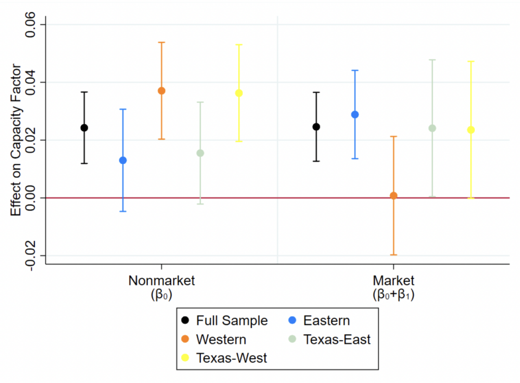
Notes: Standard errors are clustered at the plant-level.

As shown in Table 4’s binned own-drought results, allowing own-drought to vary in severity reveals that own-drought’s effects on gas-fired plants intensify with drought severity (i.e., more severe drought elicits larger capacity factor increases). For our full sample and Eastern Interconnection results, we find that market plants’ capacity factor increases are twice as large in severe drought $D_3$ than in mild drought $D_1$ . Nonmarket plants again experience the same capacity factor increases as market plants, but they do not grow as much with worsening drought severity, possibly reflecting the limitations of fleet-wide generation reoptimization or extensive bilateral trading compared to wholesale markets’ centralized transactions.

As for coal-fired plants, we find largely null drought effects for both market and nonmarket plants.⁷² However, focusing on drought-intensive years reveals the expected decreases in capacity factor for Texas market plants (Figure 7).

Figure 7. Binary Own-Drought’s Effects on Market versus Nonmarket Plants: ST-CO Capacity Factor, Drought-Intensive Years

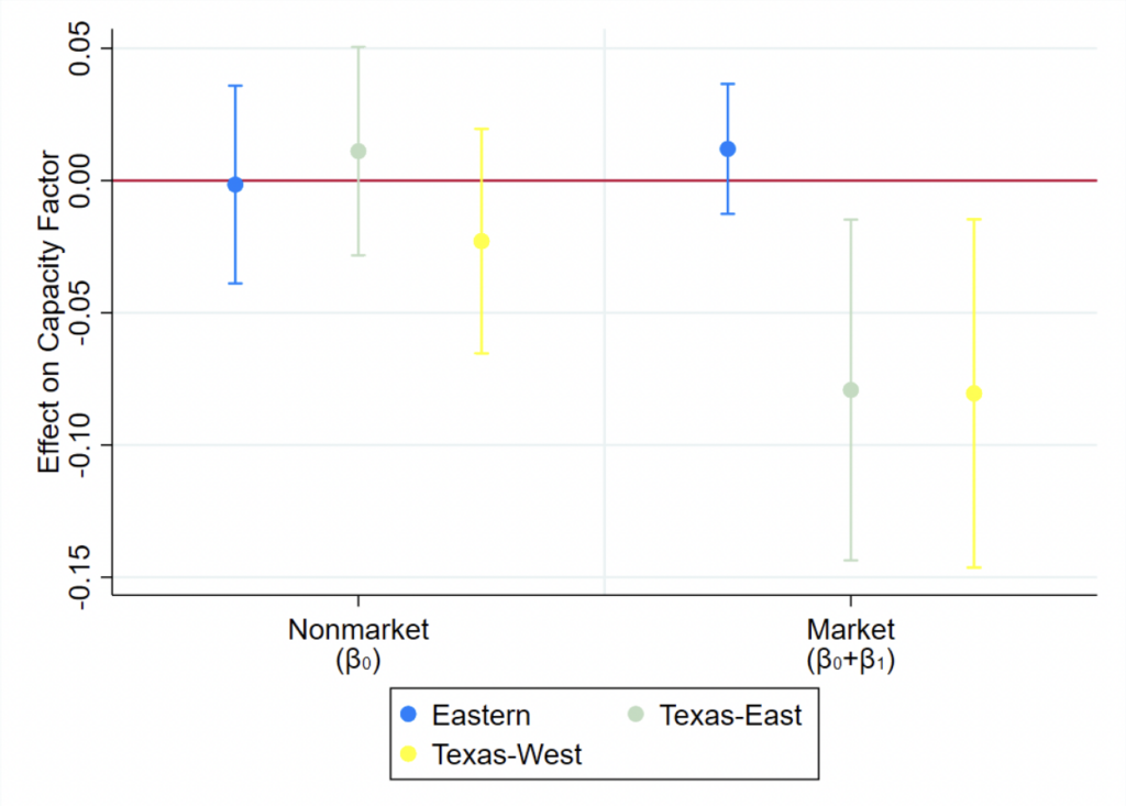
Notes: Standard errors are clustered at the plant-level.

Moreover, as shown in Table 5, allowing own-drought to vary in severity reinforces the binary drought results for Texas coal-fired market plants displayed in Figure 7. As with gas-fired market plants, worsening drought severity also has the same effect of intensifying capacity factor effects: capacity factor decreases grow in magnitude with more severe drought, with effects nearly doubling from mild to moderate drought. However, drought’s effect disappears under severe drought. Because the drought-intensive period for Texas (2018–2019) comes after an extensive period of coal-fired plant retirements and wind power increases, this result may reflect the baseload of coal generation remaining online and unaffected despite cost increases.

6.1.2 Heat Rate Results

A graphical confirmation of our market versus nonmarket plants heat rate Hypothesis H0 using binary own-drought is denoted by a dot above the zero line for nonmarket plants and below the zero line for market plants regardless of fuel type. We only find significant heat rate responses in Western Interconnection market plants, as shown in Figures 8 and 9. Figure 8 (which restricts responses to be equal across all PMFTs) shows that Western Interconnection market plants (which are all located in CAISO) decrease their heat rate when in drought. Estimating our binary drought Equation (6) by key PMFT uncovers the fact that this overall effect is driven by ST-NG units, which reduce their heat rate substantially when in drought (Figure 9).

The average heat rate of CAISO ST-NG units in our final analysis sample is approximately 20.184, well above the CAISO average of 14.170 across all plant types and the average heat rate of CAISO CC-NG units (approximately 8.034). This is consistent with the fact that ST-NG units are mostly peaker plants that mainly serve peak demand periods and are required to quickly ramp up to a certain generation level, making them much less efficient and costlier to run than their combined-cycle (CC-NG) counterparts. When these costlier units are in drought, they face stronger incentives to minimize costs through efficiency improvements than other types of plants since they are called upon to generate infrequently. That is, their opportunities to be marginal or inframarginal are few and far between compared to baseload natural gas (CC-NG) plants, which serves to intensify competition among ST-NG peakers during drought. This intensified competition manifests in the form of sizable heat rate reductions (efficiency improvements) during drought.

Figure 8. Binary Own-Drought’s Effects on Market versus Nonmarket Plants: Heat Rate, All Technologies

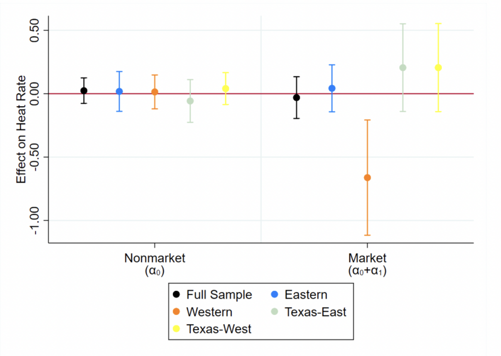
Notes: Standard errors are clustered at the plant-level.

Figure 9. Binary Own-Drought’s Effects on Market versus Nonmarket Plants: ST-NG Heat Rate

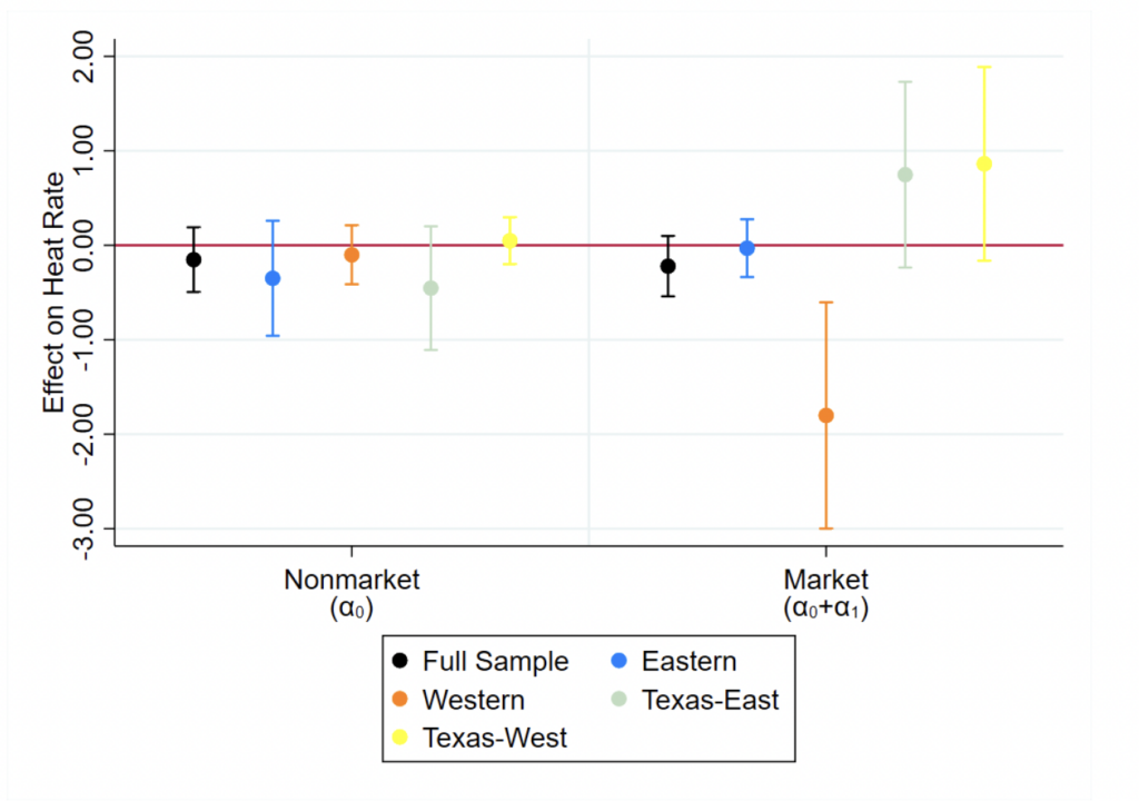
Notes: Standard erros are clustered at the plant-level.

Similar to our capacity factor results, allowing own-drought to vary in severity reveals that Western Interconnection market plants intensify their heat rate decrease under more severe drought. Considering all generating technologies equally, Table 6 shows that the heat rate decrease in Western Interconnection market plants is larger in severe drought than in mild drought, but the difference is relatively small. Focusing on binned own-drought effects on ST-NG units in Table 7 shows that similar to binary own-drought’s heat rate effects, these peaker units are driving the overall binned own-drought effects. Western Interconnection market plants decrease their heat rate by about 23 percent more in severe drought than in mild drought.

6.2 Own-Drought’s Market-Dependent Effects on Market Plants

The interpretation of the graphs in this subsection is as follows. In our binary own-drought model results, the no-drought or "D0" portion shows market-drought's effect when a plant is not in drought, and the drought or "D1" portion shows market-drought's effect when a plant is in drought (regardless of drought severity). Thus, the plotted dots in the no-drought (D0) portion are point estimates of market-drought's marginal effect when a plant is not in drought $\beta_0$ for capacity factor or $\alpha_0$ for heat rate. Meanwhile, the plotted dots in the drought (D1) portion are point estimates of market-drought's total marginal effect when a plant is in drought $(\beta_0+\beta_2)$ for capacity factor or $(\alpha_0+\alpha_2)$ for heat rate.

Moreover, in our binned own-drought model results, the no-drought or D0 bin refers to market-drought's effect when a plant is not in drought, and the D1 bin refers to market-drought's effect when a plant is in mild drought. Bin "D2" refers to market-drought's effect when a plant is in moderate drought, and "D3" refers to market-drought's effect when a plant is in severe drought. The plotted dots are therefore the point estimates of each drought bin $k$ 's respective $\beta_0$ (market-drought's effect when a plant is not in drought) or $(\beta_0+\beta_k)$ (market-drought's total marginal effect when a plant is in drought bin $D_k$ ) for capacity factor or $\alpha_0$ (market-drought's effect when a plant is not in drought) or $(\alpha_0+\alpha_k)$ (market-drought's total marginal effect when a plant is in drought bin $D_k$ ) for heat rate. The bars above and below each dot in both the binary and binned own-drought model results represent the point estimate's 95 percent confidence interval.

6.2.1 Capacity Factor Results

A graphical confirmation of our market-drought capacity factor Hypotheses H1 and H2 is denoted by a dot above the zero line in both the no-drought and drought portions of the graphs. Beginning with our binary own-drought model results, we find that market plants in our full sample and Eastern Interconnection specifications experience exactly the expected capacity factor effects when not in drought and when in drought. Specifically, an increase in market-drought when a plant is not in drought increases their capacity factor as more plants in the market get shifted up the supply curve, while a decrease in market-drought when a plant is in drought decreases their capacity factor as less of the market gets shifted up the supply curve while the plant in drought still gets shifted up. Figures 10 and 11 show this for all technologies and CC-NG units, respectively.

Figure 10. Binary Own-Drought’s Market-Dependent Effects on Capacity Factor, All Technologies

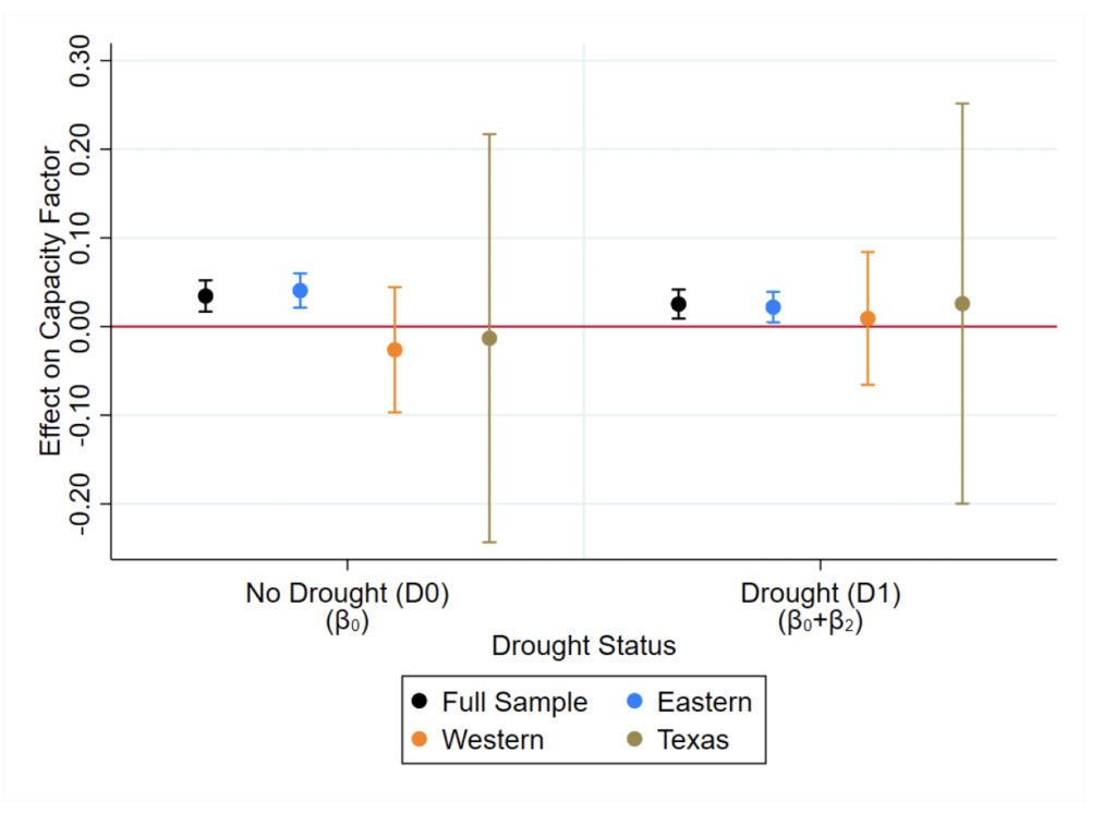
Notes: Standard errors are clustered at the plant-level.

Figure 11. Binary Own-Drought’s Market-Dependent Effects on CC-NG Capacity Factor

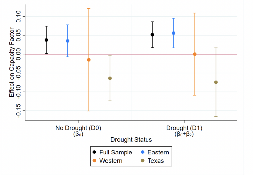
Notes: Standard errors are clustered at the plant-level.

Allowing own-drought to vary in severity for our all technologies specification shows that worsening own-drought severity potentially intensifies market-drought’s effects (Figure 12) as it did own-drought’s effects in the prior subsection, albeit meagerly and limited to our full sample estimation.

Figure 12. Binned Own-Drought’s Market-Dependent Effects on Capacity Factor, All Technologies

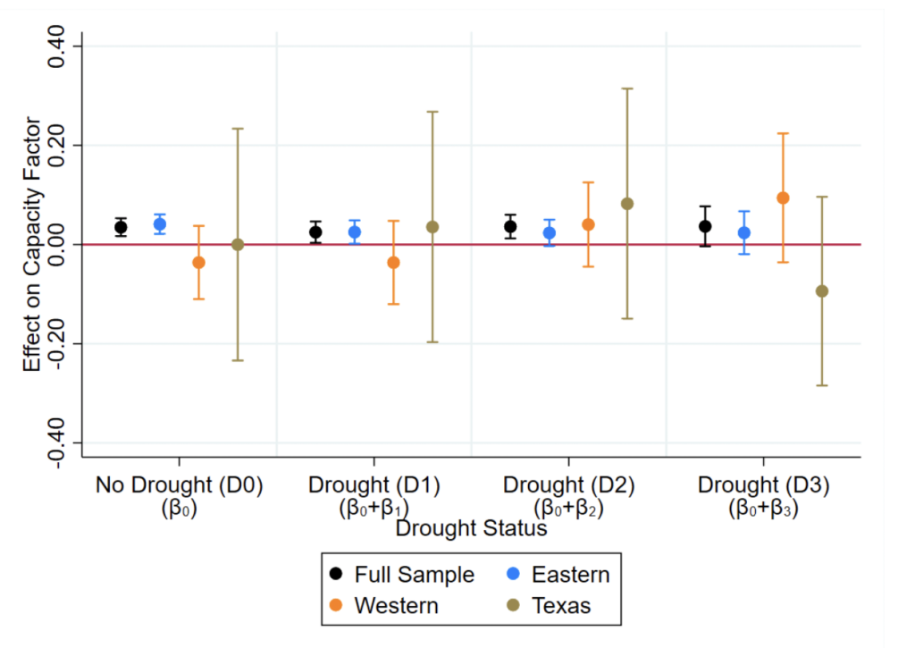
Notes: Standard errors are clustered at the plant-level.

The lack of significant responses in the Western Interconnection and Texas is likely due to those regions having less market plants with which to identify market-drought responses counts.⁷³ However, we actually find that Texas ST-CO market plants experience our expected market-drought capacity factor effects during the state’s drought-intensive years of 2018–2019 (Figure 13). Allowing own-drought to vary in severity further reveals that this effect during drought-intensive years is again present when a plant is not in drought, and it is driven solely by mild own-drought when a plant is in drought (Figure 14). These findings may indicate that coal-fired plants in Texas are especially sensitive to persistent or frequent own-drought when it interacts with market-drought conditions.

Figure 13. Binary Own-Drought’s Market-Dependent Effects on ST-CO Capacity Factor, Drought-Intensive Years

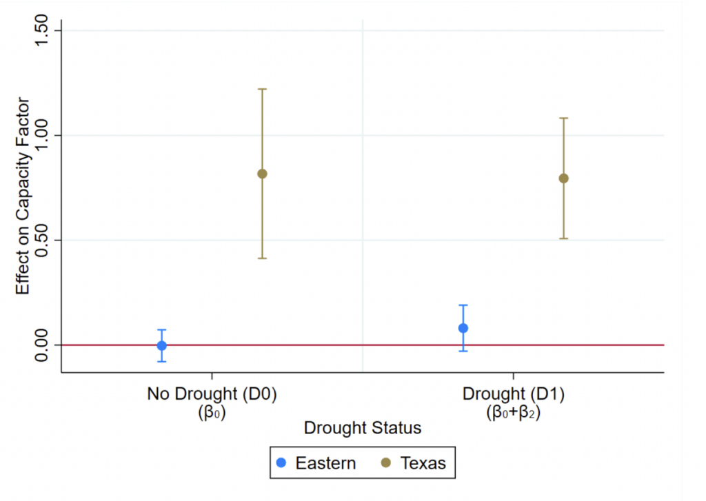
Notes: Standard errors are clustered at the plant-level.

Figure 14. Binned Own-Drought’s Market-Dependent Effects on ST-CO Capacity Factor, Drought-Intensive Years

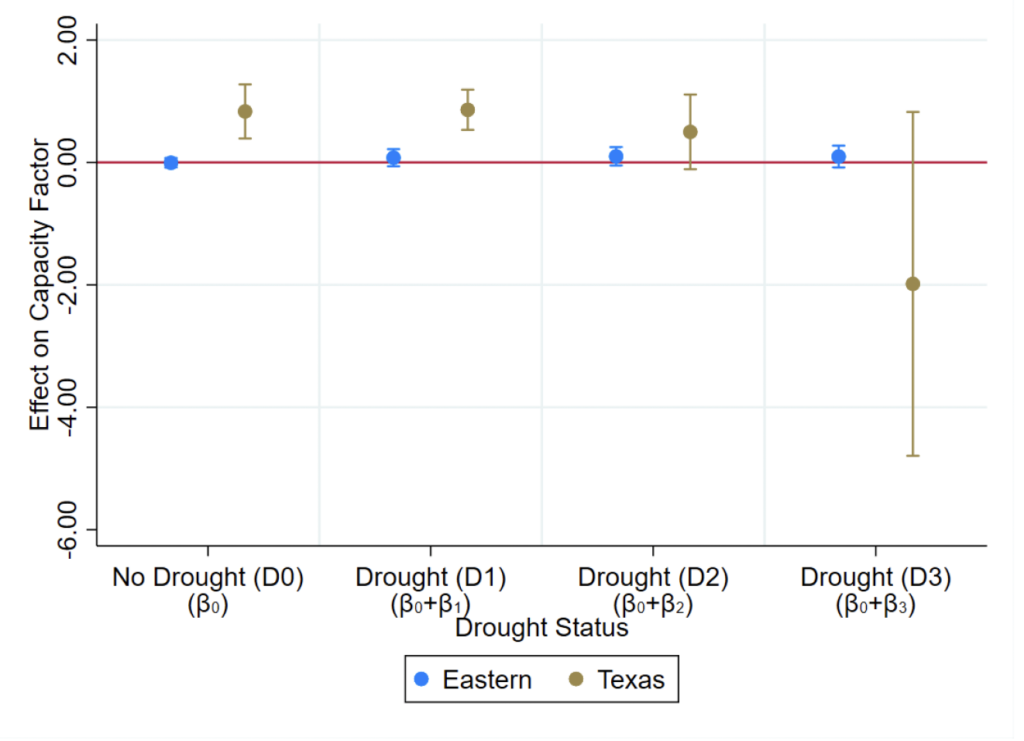
Notes: Standard errors are clustered at the plant-level.

6.2.2 Heat Rate Results

In this final subsection, a graphical confirmation of our market plant heat rate Hypotheses H1 and H2 is denoted by a dot below the zero line in the no-drought (D0) bin and a dot above the zero line in all drought bins (D1, D2, D3). We find little evidence of market plants adjusting their heat rate at all when not in drought, basically limited to CC-NG plants in Texas. We find essentially no evidence of market plants in drought decreasing their heat rate when market-drought decreases, except for ST-NG Eastern Interconnection plants in severe drought. Thus, market-drought does not appear to factor into market plants’ own-drought heat rate responses. Another factor at play for heat rate is plant planning horizons. Even with persistent or frequent drought, plants may lock in their operational expenses and strategies in blocks of months or annually, which is behavior that is masked by our monthly data and analyses.

7 Discussion

Our empirical analyses largely confirms our market versus nonmarket plant hypotheses for drought’s effects on capacity factor and heat rate. We find that natural-gas-fired market plants experience capacity factor increases when in drought, while coal-fired market plants experience capacity factor decreases when in drought, reflecting the allocative efficiency of wholesale electricity markets in shifting generation from water-intensive (coal) plants to less water-intensive plants (natural gas). Extending our analyses to include the role of market-drought reveals that only capacity factor effects are significantly affected by market-drought and consistent with our theoretical predictions; we find that nonmarket and market plants’ heat rates are mostly unresponsive to own-drought and market-drought. However, our results are greatly dependent on region and, to a lesser extent, drought frequency and persistence. This points to both statistical power issues in our sample as well as possible market failures in the Western Interconnection and Texas, where transmission issues (Buchele, 2023) combined with high levels of renewable generation (US EIA, 2023b) may be at fault.

We also find evidence of worse own-drought severity intensifying capacity factor effects. This makes sense as worsened drought conditions amount to larger cost shocks (i.e., severe drought imparts a larger efficiency loss and consequent marginal cost increase to plants than mild drought does) that should then elicit larger shifts within wholesale electricity supply curves. Our results overall highlight the importance of market structure due to the differing ways that costs are treated under different market structures.

Our results mostly extend prior research by assessing two previously unexplored channels: the role of market structure and the role of market-drought in plants’ drought responses. We can measure plant-level effects in both channels more precisely than prior work through our high-resolution PDSI data. Our work follows some previous research in studying drought’s generation effects (Mamkhezri and Torell, 2022; Qiu et al., 2023), but we use capacity factor rather than generation to account for differing plant sizes. Moreover, we follow research like Eyer and Wichman (2018) in studying large regions of the contiguous United States under the universe of drought events in our sample period rather than studying individual regions or single drought events (Scanlon et al., 2013; Mamkhezri and Torell, 2022). Finally, much of the research on the relationship between drought and thermoelectric power plants exists within the engineering literature (van Vliet et al., 2012; van Vliet, Vögele, and Rübbelke, 2013; van Vliet et al., 2016; Ganguli, Kumar, and Ganguly, 2017; Kern and Characklis, 2017). We extend the nascent and equally important research on this relationship from an economic perspective.

We also observe multiple instances of unexpected or counterintuitive results. The most notable is nonmarket plants experiencing the same capacity factor effects due to drought as market plants. The primary and most likely explanation for this is nonmarket plant operating utilities or entities engaging in fleet-wide generation reoptimization, that is, shifting their generation from water-intensive to less water-intensive plants when drought occurs by manually changing generation across their fleet. This behavior mimics the actions of a centralized wholesale electricity market, which accomplishes the same result but through a merit order based on each plant’s generation cost. Nonmarket utilities or entities may also augment their bilateral trading efforts with other nonmarket entities during drought in an effort to maintain reliability during extreme weather events.⁷⁴

The next unexpected result is the extensive absence of heat rate responses among both market and nonmarket plants. We only find significant heat rate decreases from Western Interconnection market plants, mostly from peaker ST-NG units that probably face considerably stronger incentives to remain cost-competitive than other generating units like combined-cycle natural gas or coal units. Given the prevalence of combined-cycle natural gas (CC-NG) units and the nontrivial (but waning) presence of coal (ST-CO) units in the Eastern Interconnection, we expected these units to adjust their heat rate during drought and for market-drought to significantly affect the heat rate responses of the market plants that employ CC-NG or ST-CO generation. We attribute the lack of heat rate responses to unknown power plant planning horizons. Plants’ planning horizons for responding to potentially long-lived climactic factors like drought may be longer than our analyses’ time scale of a month such that month-to-month changes may not pick up plant heat rate adjustments. Central to this planning horizon mechanism is the possibility that the benefits of not adjusting heat rate at all outweigh the benefits of adjusting heat rate in response to drought. Riding out drought may be preferable to repeatedly adjusting heat rate, particularly if heat rate adjustments are not permanent and require that costs be incurred even when drought is no longer occurring. Despite the lack of plant heat rate responses in both our market versus nonmarket and market-drought models, we still observe considerable capacity factor effects in both modeling frameworks, indicating that certain markets (particularly those in the Eastern Interconnection) are functioning properly by reordering supply curves in a cost-minimizing fashion during drought and in different market-drought conditions.

We also expected more robust results from Western Interconnection and Texas CC-NG and ST-CO plants given their frequent exposure to drought conditions compared to Eastern Interconnection plants (which experience less drought events and enjoy greater water access overall). As shown in the prior section, much of the heat rate results stem from peaker ST-NG units, although CC-NG capacity factor results tend to be more in line with our expectations. However, frequent exposure to drought may actually work against these regions in our estimation process. The plentiful null effects for our market versus nonmarket and market-drought models are likely due to poor spatial variation in drought in the Western Interconnection and Texas. Plotting the spatial distribution of PDSI (as in Figure 3) over all months in our sample reveals that areas like CAISO tend to always almost completely be in drought or not in drought, supporting the poor spatial variation channel. Furthermore, as pointed out by an anonymous reviewer, overwhelmingly large drought impacts may mask heat rate adjustments; drought may increase certain plants’ heat rate so much that no plant-level adjustments can offset it. Finally, all of our results are tempered by our empirical methodology’s chief limitation: limited modeling of drought’s possibly nonlinear effects on plant operations.

In addition to increasing the amount of renewable energy on the grid, policy-based efforts to decarbonize the energy sector also include changes to the thermoelectric fleet such as plant retirements (mainly for coal-fired plants), retrofits (e.g., modifying coal plants to run on natural gas), and stricter emissions standards. These changes are especially important to consider in the context of drought as reliability concerns mount with the increasing frequency of extreme weather events in general. Policymakers are increasingly concerned with the fossil-fuel fleet’s ability to withstand extreme heat and cold events since this ability can impact the wholesale price of electricity and consequently affect retail electricity prices.⁷⁵ Our results show that thermoelectric plants’ drought responses are dependent upon fuel type (by way of water intensiveness) and region. That is, some areas’ markets appear to be functioning as intended when it comes to plant cost minimization in the face of extreme weather, but this result is specific to certain fuels and generating technologies. For example, we find that coal-fired plants tend to display significant effects only in drought-intensive years. This points to a need for policy to not only be area specific but also technology specific and weather dependent.

The importance of the dichotomy between competitive and noncompetitive market structures for electricity that we uncover is also relevant for policies aiming to incentivize extreme weather responses for power plants. A blanket policy for all natural-gas-fired power plants regardless of the type of market that they operate in, for example, would potentially limit the policy’s efficacy by allowing advantageous strategic compliance or efficiency losses due to differing market mechanisms. This is especially pertinent for nonmarket regions whose operating entities appear to mimic market areas in our results, since such regions may be well suited for market-based policies despite not formally operating a competitive wholesale market.⁷⁶ Moreover, the apparent irrelevance of market-drought for plant-level heat rate adjustments that we find underscores the fact that own-drought is the only salient factor for plant-level decisions. That is, while our market-drought capacity factor results enhance our market versus nonmarket analyses by showing that markets are working as intended even in the face of market-level cost shocks, plants do not appear to account for such market-level drought impacts when making plant-specific decisions (capacity factor is largely a function of market forces and the merit order, not plant-level decisions). Thus, policies could benefit from focusing on regulating market-level operations rather than on plant-level regulatory approaches. Improving and expanding market mechanisms for wholesale power may ultimately spur greater grid resilience and efficiency than relying on plant-specific adjustments.⁷⁷

8 Conclusion

The transition to a decarbonized energy sector is a major part of society’s efforts to adapt to and mitigate climate change. This transition will take time to occur as renewable generating technologies are implemented, and therefore the behavior of existing fossil fuel plants takes center stage as extreme weather events (like drought) increase in frequency. Thus, it is important to understand how these plants respond to drought, whether electricity markets affect their responses in an efficient cost-minimizing manner, and how the extent of drought affects such responses. Prior work has studied generation responses without considering market structure, but we contribute additional perspectives by studying efficiency responses, responses in different market types (competitive markets versus nonmarket monopolistic utilities), and explicitly modeling the dependence of plant drought responses on market-drought conditions.

We use panel data on thermoelectric power plants’ operations and a novel high-resolution PDSI data set along with fixed effects regression models to examine whether wholesale electricity markets enact the expected capacity factor (generation reallocation) and efficiency (heat rate improvement by market plants) effects and how generating units respond to their own-drought condition under different market-drought conditions. The essence of our drought response framework lies in the fact that drought ultimately decreases plant efficiency and increases marginal cost in the absence of any adjustment by the plant. Our theoretical exposition on market plants versus nonmarket plants posits that market areas should engage in generation reallocation from water-intensive (coal) plants to less water-intensive (natural gas) plants and incentivize market plants to improve their efficiency (reduce their heat rate) during drought. In addition, nonmarket plants are not expected to experience either outcome.

Next, focusing on market plants, our theoretical market-drought exposition predict that plants’ drought responses along two margins (capacity factor and heat rate) depend on the extent of market-drought in their area. Plants in drought are expected to experience capacity factor decreases only if market-drought is relatively low. This is because lower market-drought corresponds to less of the market supply curve being shifted, leaving the plant that is in drought with greater losses in their probability of being inframarginal or marginal (i.e., of generating). Plants not in drought are expected to experience capacity factor increases only if market-drought is relatively high. This is because higher market-drought means that more of the plants in the market are shifted up the supply curve, which increases the probability of a plant not in drought being inframarginal or marginal. As for heat rate, plants in drought are expected to not lower their heat rate in response to drought if market-drought is high. This is because more of the supply curve is shifted up with the plant in drought when market-drought is high, eroding the incentives for such a plant to reduce its heat rate.

Through our econometric analyses, we generally find that market plants experience the capacity factor effects and, to a lesser extent, exhibit the heat rate improvements that we expect market areas to incentivize. However, these results depend on region, with capacity factor effects largely only appearing in the Eastern Interconnection and heat rate responses only appearing in the Western Interconnection. Our results also highlight peaker ST-NG plants as being especially sensitive to drought with respect to heat rate or efficiency adjustments. Our market-drought effects are quite muted for capacity factor (with minute effects again limited to Eastern Interconnection plants) and almost nonexistent for heat rate, indicating that only own-drought conditions matter for plant-level efficiency adjustments during drought. Moreover, many of our binned own-drought results display evidence of worsening drought severity intensifying capacity factor effects. Finally, drought persistence and frequency only factor into plant responses in a few market-technology scenarios, as evidenced by our limited significant results from focusing on drought-intensive years.

This paper’s theoretical framework and empirical results accentuate the need for area-specific and technology-specific policy within the water-energy nexus, particularly as it pertains to wholesale and retail costs within the greater scope of reliability. Effective electric reliability or cost-effectiveness policy likely cannot take any sort of blanket approach if efficiency and cost minimization are to be central tenets. As recent efforts to modernize and retrofit fossil fuel plants amid mounting reliability concerns have shown, policymakers are increasingly concerned with such plants’ ability to endure extreme weather events for the sake of providing power and ideally providing it at least cost. Competitive electricity markets are supposed to accomplish just that. We find that some areas’ markets are functioning as intended and incentivizing the right plants to generate more or less and improve their efficiency under drought. Interestingly, nonmarket plants are experiencing the same capacity factor effects as their market counterparts, which, combined with the results for market plants, emphasizes the dichotomy between competitive and noncompetitive market structures for electric policy; even nonmarket entities may be open to engaging in electricity markets.

Finally, the fact that market-drought matters for plant capacity factor points to the potential for expanded grid transmission to help with extreme weather resilience. Ongoing transmission expansion efforts can benefit from this research’s insights, particularly since we lack robust results in the Western Interconnection and Texas (which are both ridden with transmission issues). Transmission expansion can further the growth of wholesale electricity markets or even just market-reminiscent structures like the nascent Southeastern Energy Exchange Market, enabling increased access to the generation reallocation that we find in this paper.

Although our analyses use drought data at a high spatial resolution that allows us to construct IDW plant-level drought conditions, we still may not be capturing drought’s effects as accurately as possible. This is because a plant’s true drought conditions may only depend on the water supply in their cooling water source. Future research should explore the incorporation of hydrological models to better characterize true drought conditions at individual plants. In addition, our attempt at modeling nonlinear drought effects through drought bins may not be ideal. Future research should attempt to explicitly model such nonlinear effects.

Regression Tables

Appendix A: Drought’s Effects on Power Plant Efficiency and Marginal Cost

Thermoelectric power plants generate electricity by combusting a fossil fuel (e.g., coal or natural gas) and using the resulting heat to create steam that is then passed through a turbine to turn its blades and the rotor shaft of a generator, which then generates electricity. After passing through the turbine, the steam must then be cooled back into liquid form to be reused in the second step of the aforementioned process. Outside water must be withdrawn from a surface water source (or cooling tower in recirculating cooling systems⁷⁸) to be used as cooling water in plants’ cooling systems and the steam cooling process.

Figure 15 illustrates the generation and water usage processes for a plant with a recirculating cooling system (as evidenced by the presence of a cooling tower).⁷⁹ A crucial component of a thermoelectric power plant’s cooling system is its condenser, which serves as a heat rejection mechanism for cooling/condensing used steam back into liquid form for reuse in the electricity generation process (Zubovic, 2021). Not only do condensers cool steam back into liquid form, but they also create a pressure sink that helps pull steam through the turbine. This affects the generation capacity of the turbine/generator (Zubovic, 2021) and consequently impacts the efficiency of the electricity generation process, which we elaborate on below.

Figure A1. Illustration of How Generation andWater Usage Occurs at Thermoelectric Power Plants

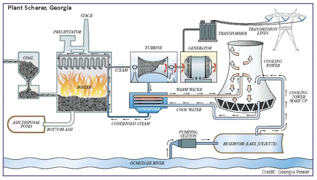
Notes: Figure source is US Geological Survey Water Science School (2018).

From an engineering perspective, drought’s water quantity and quality (temperature) effects chiefly affect the condenser’s operating conditions. The most important condenser condition parameter is condenser pressure, which is increased by both higher intake water temperatures (quality effect) and lower streamflow (quantity effect) (Putman and Harpster, 2000; Pattanayak, Padhi, and Kodamasingh, 2019). An increase in condenser pressure amounts to an increase in the endpoint pressure on the exhaust side of the turbine (since the cooling system is the first place that exhaust steam travels to after passing through the turbine, hence the endpoint term; the condenser is the endpoint for the plant’s water cycle). Continuing with the pressure sink terminology, this means that an increase in condenser pressure shrinks the sink, reducing its ability to pull steam through the turbine.⁸⁰ Absent an adjustment by the turbine, this rise in endpoint (or condenser) pressure reduces the generating capacity of the turbine as well as the generation level (i.e., less energy can be extracted from the same steam since it is moving through the turbine more slowly due to the sink shrinkage).

In practice, turbines do adjust to this rise in endpoint pressure: the turbine governor, which regulates the turbine’s rotational speed (Petrotech, 2017), increases the throttle to increase the steam flow (Lakovic et al., 2010; Pattanayak, Padhi, and Kodamasingh, 2019) and maintain the generation level. To achieve this increased steam flow, the fuel firing rate is increased (Lakovic et al., 2010), meaning that more fuel is combusted to generate the same amount of electricity. Recalling that heat rate (our measure of efficiency) is equal to the amount of fuel combusted divided by the amount of electricity generated, this result means that the heat rate has increased and efficiency has decreased due to the increase in condenser pressure. Other research that confirms this negative relationship between condenser pressure and efficiency includes Bhoi, Meta, and Bhojak (2015) and Hamanaka, Zhao, and Sharpe (2009).

Colman (2013) provides another avenue through which plant efficiency is affected by drought’s quality (temperature) effect by connecting increased intake water temperature with a heat engine’s Carnot efficiency. Carnot efficiency is the maximum possible efficiency achievable by a heat engine operating between two temperatures (Pisupati, 2020): a heat source temperature $T_H$ (i.e., steam temperature) and a heat sink temperature $T_C$ (i.e., cooling water temperature). Letting $Q_H$ be the heat input (i.e., fuel combusted), $Q_C$ be waste heat dissipated, and $W$ be work done (i.e., MWh of electricity generated), let thermal efficiency be

$\eta_{t h}=\frac{W}{Q_H}$

By the first law of thermodynamics, and the fact that energy cannot be completely converted to work $W$ , the heat input (fuel combusted) $Q_H$ must equal work done plus waste heat dissipated, meaning that

$\begin{gathered}Q_H=W+Q_C, \W=Q_H-Q_C .\end{gathered}$

Thus, thermal efficiency can be rewritten as

$\eta_{t h}=\frac{Q_H-Q_C}{Q_H}.$

Simplifying the equation for thermal efficiency and letting $T_C = Q_C$ , $T_H = Q_H$ be the temperatures of the heat sink (condenser) and heat source (steam), respectively, we obtain the equation for Carnot efficiency $\eta_C$ :

$\eta_C=1-\frac{T_C}{T_H}.$

Thus, for an increase in heat sink (condenser) temperature $T_C$ (from an increase in intake water temperature due to drought), the maximum possible or Carnot efficiency decreases.

Appendix B

Figure B1. Map of US Balancing Authorities

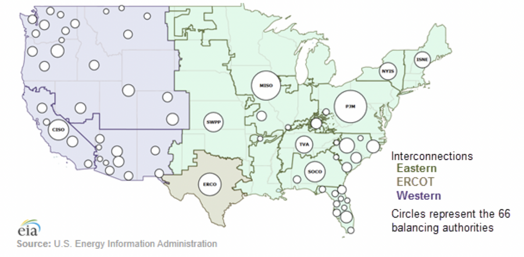
Notes: Figure source is US EIA (2016).

Appendix C

Figure C1. Map of Balancing Authority Areas in the Western Interconnection

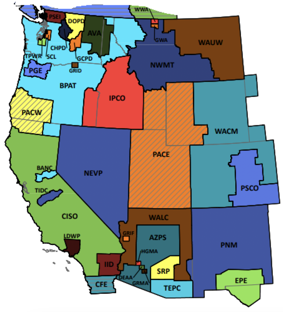
Notes: Figure source is Western Electricity Coordinating Council (2017).

Appendix D

Figure D1. Example of Electricity Dispatch Curve with Perfectly Inelastic Demand Curves

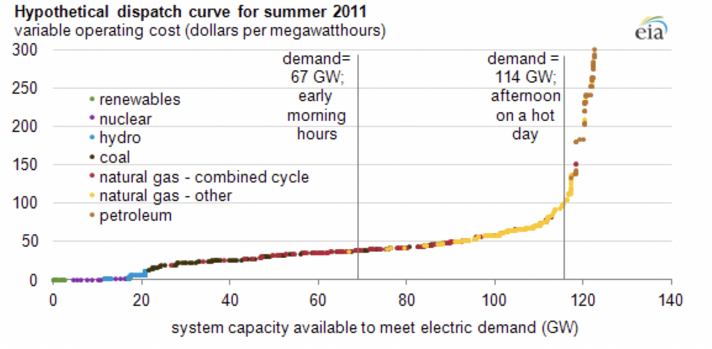
Notes: Figure source is US EIA (2012).

Appendix E

Once-through systems withdraw water, use it in the cooling process, and discharge it (at a warmer temperature) back to its source. Such systems are widespread across the eastern United States and were popular due to their low cost and simplicity (Union of Concerned Scientists, 2013). Recirculating systems withdraw water but at much lower volumes and rates than once-through systems because they use cooling towers or ponds to reuse withdrawn cooling water. These towers or ponds expose used cooling water to ambient air to cool it; some cooling water naturally evaporates as a result, and the remaining cooling water is reused in the steam cooling process (Union of Concerned Scientists, 2013). Consequently, recirculating systems have much higher water consumption volumes and rates than once-through systems (US EIA, 2014). Dry cooling systems use ambient air to cool steam, and can be categorized into two types: direct systems that use no water at all and indirect systems that use minimal cooling water kept in a closed system. Finally, hybrid cooling systems are a blend of dry and wet cooling.

Appendix F: Select Results Using County-Level PDSI for Own-Drought (gridMET PDSI for Market-Drought)

Figure F1. County-Level Binary Own-Drought’s Effects on Market versus Nonmarket Plants: CC-NG Capacity Factor

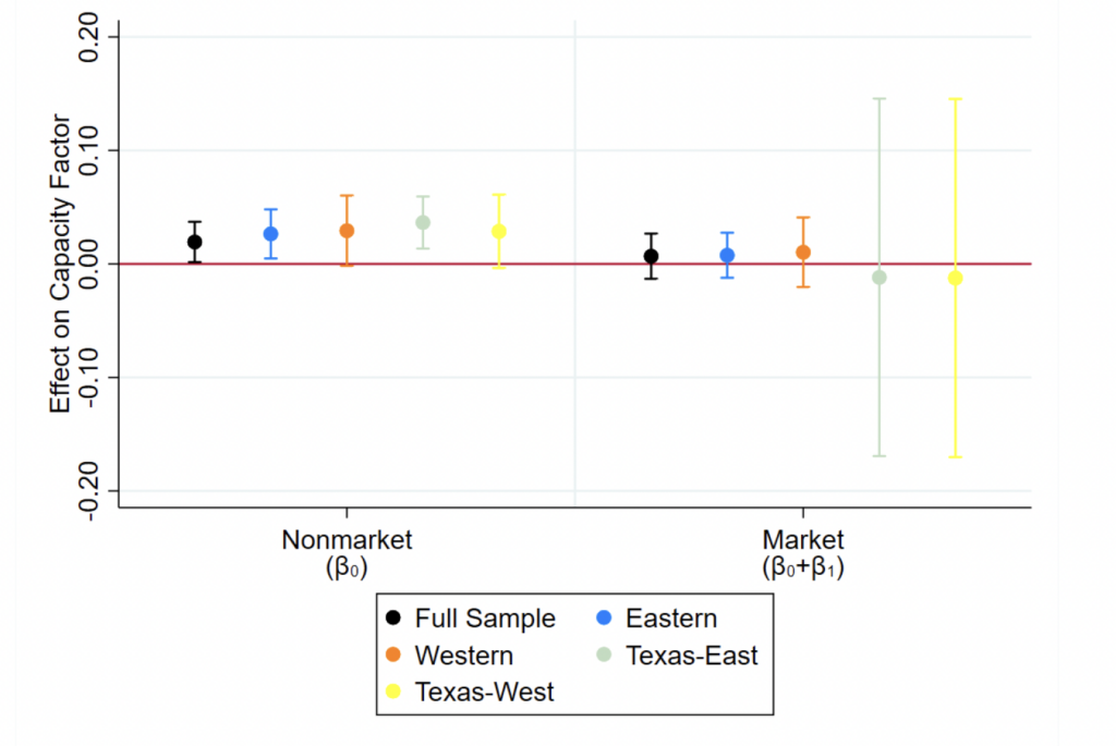
Notes: Standard errors are clustered at the plant-level.

Figure F2. County-Level Binary Own-Drought’s Market-Dependent Effects on CC-NG Capacity Factor

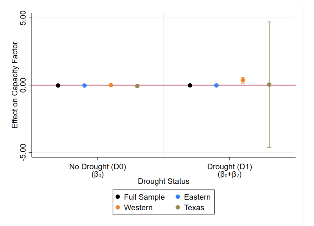
Notes: Standard errors are clustered at the plant-level.

Figure F3. County-Level Binary Own-Drought’s Market-Dependent Effects on Capacity Factor, All Technologies

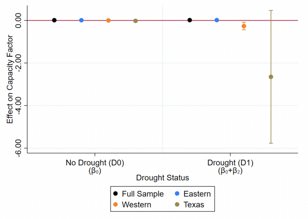
Notes: Standard errors are clustered at the plant-level.

Figure F4. County-Level Binary Own-Drought’s Effects on Market versus Nonmarket Plants: Heat Rate, All Technologies

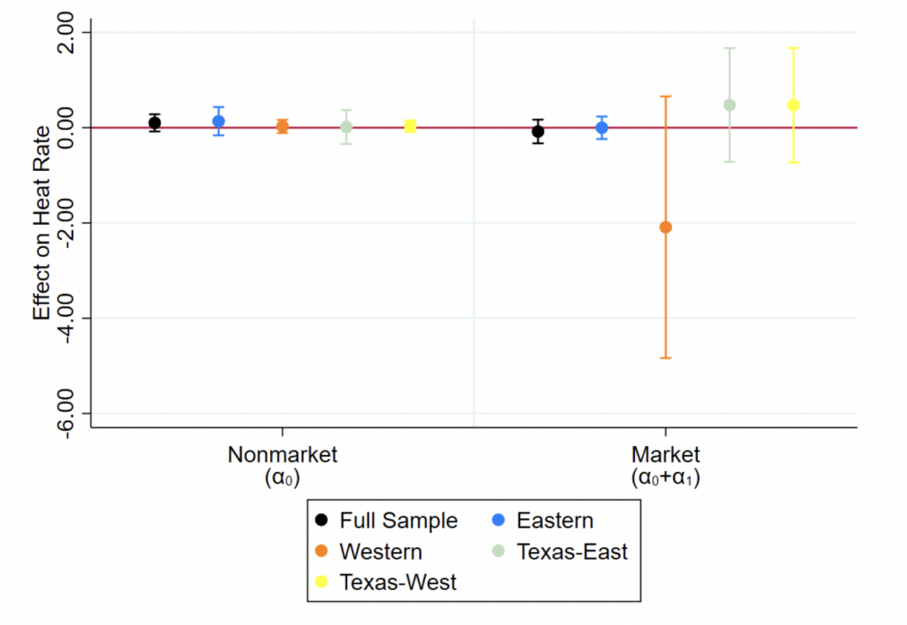
Notes: Standard errors are clustered at the plant-level.

Figure F5. County-Level Binary Own-Drought’s Market-Dependent Effects on CC-NG Heat Rate

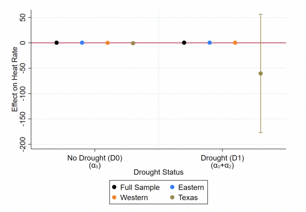
Notes: Standard errors are clustered at the plant-level.

References

Bartos, M.D. and M.V. Chester. 2015. “Impacts of Climate Change on Electric Power Supply in the Western United States,” Nature Climate Change, 5(8), 748–752.

Bhoi, R., N. Meta, and K. Bhojak. 2015. “Effect of Condenser Backpressure on Power Plant Heat Rate and Thermal Efficiency,” International Journal for Scientific Research & Development, 3(1).

Bogmans, C.W.J., G.P.J. Dijkema, and M.T.H. van Vliet. 2017. “Adaptation of Thermal Power Plants: The (Ir)relevance of Climate (Change) Information,” Energy Economics, 62, 1–18.

Buchele, M. 2023. “ERCOT Can’t Move Energy Where It Needs to Go, and It’s Putting the Grid at Risk,” KUT News.

Byers, E.A., G. Coxon, J. Freer, and J.W. Hall. 2020. “Drought and Climate Change Impacts on Cooling Water Shortages and Electricity Prices in Great Britain,” Nature Communications, 11.

Chandel, M.K., L.F. Pratson, and R.B. Jackson. 2011. “The Potential Impacts of Climate- Change Policy on Freshwater Use in Thermoelectric Power Generation,” Energy Policy, 39, 6234-6242.

Colman, J. 2013. “The Effect of Ambient Air and Water Temperature on Power Plant Efficiency,” Duke University Master’s Thesis.

Denooyer, T.A. 2015. “Integrating Water Resources and Power Generation: The Energy-Water Nexus in Illinois,” University of Illinois at Urbana-Champaign Master’s Thesis.

DiSavino, S. and S. Kelly. 2021. “Texas Power Consumers to Pay the Price of Winter Storm,” Reuters.

Doran, L. 1997. “Steam Traps Affect Boiler Plant Efficiency,” National Board BULLETIN. https://www.nationalboard.org/index.aspx?pageID=164&ID=229. Accessed May 6, 2022.

Doyle, M. and H. Fell. 2018. “Fuel Prices, Restructuring, and Natural Gas Plant Operations,” Resource and Energy Economics, 52, 153–172.

Drought.gov. n.d. “Drought Basics,” https://www.drought.gov/what-is-drought/droughtbasics. Accessed November 21, 2022.

Einberger, M. 2023. “Reality Check: The United States Has the Only Major Power Grid without a Plan,” RMI.

Eyer, J. and C.J. Wichman. 2018. “Does Water Scarcity Shift the Electricity Generation Mix toward Fossil Fuels? Empirical Evidence from the United States,” Journal of Environmental Economics and Management, 87, 224–241.

Feinstein, L., and E. de Place. 2020. “Playing Monopoly; Or, How Utilities Make Money,” Sightline Institute. https://www.sightline.org/2020/05/18/playing-monopoly-or-howutilities-make-money/. Accessed May 8, 2022.

Fonseca, F.R., M. Craig, P. Jaramillo, M. Berges, E. Severnini, A. Loew, H. Zhai, Y. Cheng, B. Nijssen, N. Voisin, and J. Yearsley. 2021. “Effects of Climate Change on Capacity Expansion Decisions of Electricity Generation Fleet in the Southeast U.S.,” Environmental Science and Technology, 55, 2522–2531.

Ganguli, P., D. Kumar, and A.R. Ganguly. 2017. “US Power Production at Risk from Water Stress in a Changing Climate,” Scientific Reports, 7.

GE Gas Power. n.d. “Combined Cycle Power Plant: How ItWorks,” https://www.ge.com/gaspower/resources/education/combined-cycle-power-plants. Accessed November 21, 2022.

Golombek, R., S.A.C. Kittelsen, and I. Haddeland. 2011. “Climate Change: Impacts on Electricity Markets in Western Europe,” Climatic Change, 113, 357–370.

Hamanaka, B. H. Zhao, and P. Sharpe. 2009. “Comparison of Advanced Cooling Technologies Efficiency Depending on Outside Temperature,” Idaho National Laboratory Report DE-AC07-05ID14517.

Henry, C.L. and L.F. Pratson. 2016. “Effects of Environmental Temperature Change on the Efficiency of Coal- and Natural Gas-Fired Power Plants,” Environmental Science & Technology, 50, 9764–9772.

Henson, B. 2021. “Climate Change May Have Worsened Deadly Texas Cold Wave, New Study Suggests,” The Washington Post. Accessed November 1, 2022.

Hite, D. 2013. “Improve Plant Heat Rate with Feedwater Heater Control,” POWER Magazine. Accessed May 5, 2022.

Hunt, J. 2007. “Gas Turbine Plant Efficiency: Balancing Power, Heat, and Operational Flexibility,” Power Engineering International. https://www.powerengineeringint.com/coal-fired/equipment-coal-fired/gas-turbine-plant-efficiency-balancing-power-heat-and-operational-flexibility/. Accessed May 6, 2022.

Jaffe, M. 2023. “Why Was Your Utility Bill So High This Past Winter? Blame the Drought—and California,” The Colorado Sun.

Kambaladinne, R. 2015. “Heat Rate Reduction in Thermal Power Generation Plants Leveraging ‘Big Data/Analytics’ Solutions,” energycentral. https://energycentral.com/c/pip/heatrate-reduction-thermal-power-generation-plants-leveraging-big-data-analytics. Accessed February 8, 2023.

Kern, J.D. and G.W. Characklis. 2017. “Evaluating the Financial Vulnerability of a Major Electric Utility in the Southeastern US to Drought under Climate Change and an Evolving Generation Mix,” Environmental Science & Technology, 51, 8815–8823.

Kibbey, J.C. 2021. “Utility Accountability 101: How Do Utilities Make Money?,” Natural Resources Defense Council. https://www.nrdc.org/experts/jc-kibbey/utilityaccountability-101-how-do-utilities-make-money#::text=Here’s%20the%20basic%20idea%20behind,provide%20energy%20services%20to%20customers. Accessed May 8, 2022.

Kimmell, T.A. and J.A. Veil. 2009. “Impact of Drought on US Steam Electric Power Plant Cooling Water Intakes and Related Water Resource Management Issues,” National Energy Technology Laboratory Report.

Korellis, S. 2022. “Utilities and Industry Continue Learnings around Benefits of Heat Rate Improvement,” POWER Magazine. Accessed June 28, 2023.

Lakovic, S.M., M.M. Stojiljkovic, S.V. Lakovic, V.P. Stefanovic, and D.D. Mitrovic. 2010. “Impact of the Cold End Operating Conditions on Energy Efficiency of the Steam Power Plants,” Thermal Science, 14, 53–66.

Lashof, D.A., S. Yeh, D. Doniger, S. Carter, and L. Johnson. 2013. “Closing the Power Plant Carbon Pollution Loophole: Smart Ways the Clean Air Act Can Clean Up America’s Biggest Climate Polluters.” NRDC Report 12-11-A.

Linn, J., E. Mastrangelo, and D. Burtraw. 2014. “Regulating Greenhouse Gases from Coal Power Plants under the Clean Air Act,” Journal of the Association of Environmental and Resource Economists, 1(1), 97–134.

Maize, K. 2018. “Power Plant Efficiency: A Key to Profitable Performance,” POWER Magazine. Accessed May 5, 2022.

Mamkhezri, J. and G.L. Torell. 2022. “Assessing the Impact of Exception Drought on Emissions and Electricity Generation,” The Energy Journal, 43(4), 159–212.

McCall, J., J. MacKnick, and D. Hillman. 2016. “Water-Related Power Plant Curtailments: An Overview of Incidents and Contributing Factors,” National Renewable Energy Laboratory Technical Report NREL/TP-6A20-67084.

McClintock, M. 2018a. “Controllable Loss Monitors,” Fossil Consulting Services, Inc., https://www.fossilconsulting.com/2018/11/09/controllable-loss-monitors/#::text=A%20controllable%20parameter%20can%20be,be%20considered%20a%20controllable%20parameter. Accessed November 1, 2022.

McClintock, M. 2018b. “Keys to Improving Power Plant Efficiency,” Fossil Consulting Services, Inc., https://www.fossilconsulting.com/2018/03/08/power-plant-efficiency/. Accessed June 28, 2023.

McDermott, G.R. and O.A. Nilsen. 2014. “Electricity Prices, River Temperatures, and Cooling Water,” Land Economics, 90(1), 131–148.

National Center for Atmospheric Research. 2022. “Palmer Drought Severity Index (PDSI),” https://climatedataguide.ucar.edu/climate-data/palmer-drought-severity-index-pdsi. Accessed November 1, 2022.

National Drought Mitigation Center. 2022. “Types of Drought,” https://drought.unl.edu/Education/DroughtIn-depth/TypesofDrought.aspx#::text=Hydrological%20Drought,-Hydrological%20drought%20is%20associated%20with. Accessed November 21, 2022.

NERC Resources Subcommittee. 2011. “Balancing and Frequency Control.” NERC Technical Report.

Northern Great Plains Water Consortium. 2022. “Thermoelectric Power Plants,” https://undeerc.org/Water/Energy-Water-Nexus/Thermoelectric-Power-Plants.aspx#::text=Approximately%2089%25%E2%80%9390%25%20of,produced%20by%20thermoelectric%20power%20plants. Accessed November 17, 2022.

Patel, S. 2022. “NERC Warns of Mounting Reliability Risks, Urges Preparation for Challenging Summer,” POWER Magazine. Accessed May 5, 2022.

Pattanayak, L., B.N. Padhi, and B. Kodamasingh. 2019. “Thermal Performance Assessment of Steam Surface Condenser,” Case Studies in Thermal Engineering, 14.

Pechan, A. and K. Eisenack. 2014. “The Impact of HeatWaves on Electricity Spot Markets,” Energy Economics, 43, 63–71.

Petrakopoulou, K. 2021. “Defining the Cost of Water Impact for Thermoelectric Power Generation,” Energy Reports, 7, 2101–2112.

Petrotech. 2017. “What Is the Function of a Governor in a Steam Turbine?,” https://petrotechinc.com/what-is-the-function-of-a-governor-in-a-steam-turbine/#::text=A%20steam%20turbine%20governor%20is,steam%20flow%20to%20the%20turbine. Accessed February 18, 2023.

Pisupati, S. 2020. “The Carnot Efficiency,” Pennsylvania State University John A. Dutton e-Education Institute, EGEE 102 Energy Conservation for Environmental Protection, https://www.e-education.psu.edu/egee102/node/1942#::text=The%20Carnot%20Efficiency%20is%20the%20theoretical%20maximum%20efficiency,low%20temperature%20reservoir%20operates%20%28%20T%20Cold%20%29. Accessed February 18, 2023.

Putman, R.E. and J.W. Harpster. 2000. “The Economic Effects of Condenser Backpressure on Heat Rate, Condensate Subcooling and Feedwater Dissolved Oxygen,” Proceedings of ASME International Joint Power Generation Conference, Miami.

Qiu, M., N. Ratledge, I.M.L. Azevedo, N.S. Diffenbaugh, and M. Burke. 2023. “Drought Impacts on the Electricity System, Emissions, and Air Quality in the Western United States,” PNAS, 120(28).

Reimers, A. 2018. “Making Electricity Consumers a Lot of Water—What’s the Best Way to Fix That?,” Scientific American.

Reuters. 2021. “California Drought Cuts Hydropower, Boosts Natgas Prices.” https://www.reuters.com/business/energy/california-drought-cuts-hydropower-boosts-natgas-prices-2021-05-21/. Accessed June 29, 2023.

Reuters. 2023. “US power grids vulnerable to extreme heat conditions this summer, NERC says,”. https://www.reuters.com/business/energy/us-power-grids-vulnerable-extreme-heat-conditions-this-summer-nerc-2023-05-17/.

Scanlon, B.R., I. Duncan, and R.C. Reedy. 2013. “Drought and the water-energy nexus in Texas,” Environmental Research Letters, 8.

Simon, J. 2022. “Drought Threatens Coal Plant Operations—and Electricity—across the West,” NPR. Accessed August 26, 2022.

Stillwell, A.S., M.E. Clayton, and M.E. Webber. 2011. “Technical Analysis of a River Basin-Based Model of Advanced Power Plant Cooling Technologies for MitigatingWater Management Challenges,” Environmental Research Letters, 6.

Sustainable FERC Project. 2020. “RTO Backgrounders.” https://sustainableferc.org/rtobackgrounders-2/. Accessed October 16, 2023.

Tyran, B. 2023. “Extreme Weather Events Are Expanding—The US Power Grid Is Not,” Utility Dive.

Union of Concerned Scientists. 2013. “How It Works: Water for Power Plant Cooling,” https://www.ucsusa.org/resources/water-power-plant-cooling. Accessed November 17, 2022.

US Energy Information Administration (EIA). 2012. “Electric Generator Dispatch Depends on System Demand and the Relative Cost of Operation,” https://www.eia.gov/todayinenergy/detail.php?id=7590. Accessed November 23, 2022.

US Energy Information Administration (EIA). 2014. “Many Newer Power Plants Have Cooling Systems That Reuse Water,” https://www.eia.gov/todayinenergy/detail.php?id=14971. Accessed October 16, 2023.

US Energy Information Administration (EIA). 2016. “US Electric System Is Made Up of Interconnections and Balancing Authorities,” https://www.eia.gov/todayinenergy/detail.php?id=27152. Accessed August 26, 2022.

US Energy Information Administration (EIA). 2018. “Some US Electricity Generating Plants Use Dry Cooling,” https://www.eia.gov/todayinenergy/detail.php?id=36773. Accessed November 17, 2022.

US Energy Information Administration (EIA). 2021. “Table 8.2. Average Tested Heat Rates by Prime Mover and Energy Source, 2011–2021,” https://www.eia.gov/electricity/annual/html/epa_08_02.html. Accessed November 21, 2022.

US Energy Information Administration (EIA). 2022. “Electricity Explained: Electricity in the United States,” https://www.eia.gov/energyexplained/electricity/electricity-in-the-us.php. Accessed November 17, 2022.

US Energy Information Administration (EIA). 2023a. “US Electric Power Sector Continues Water Efficiency Gains,” https://www.eia.gov/todayinenergy/detail.php?id=56820#::text=Natural%20gas%20plants%20use%20a,making%20them%20less%20water%20intensive. Accessed November 2, 2023.

US Energy Information Administration (EIA). 2023b. “Solar and Wind Power Curtailments Are Rising in California,” https://www.eia.gov/todayinenergy/detail.php?id=60822#::text=Congestion%2Drelated%20curtailments%20have%20increased,outpacing%20upgrades%20in%20transmission%20capacity.&text=In%202022%2C%20CAISO%20curtailed%202.4,of%20electricity%20curtailed%20in%202021. Accessed November 7, 2023.

US Environmental Protection Agency. 2022. “eGRID Power Profiler,” https://www.epa.gov/egrid/power-profiler#/. Accessed November 18, 2022.

US Environmental Protection Agency. 2023a. “Climate Change Indicators: Heat Waves,” https://www.epa.gov/climate-indicators/climate-change-indicators-heat-waves. Accessed July 22, 2023.

US Environmental Protection Agency. 2023b. “US Grid Regions,” https://www.epa.gov/green-power-markets/us-grid-regions#::text=The%20U.S.%20grid%20is%20divided,The%20Texas%20Interconnected%20system. Accessed October 25, 2023.

US Geological Survey Water Science School. 2018. “A Coal-Fired Thermoelectric Power Plant.” https://www.usgs.gov/special-topics/water-science-school/science/a-coal-fired-thermoelectric-power-plant.

Van Loon, A.F. 2015. “Hydrological Drought Explained,” WIREs Water, 2, 359–392.

van Vliet, M.T.H., J.R. Yearsley, F. Ludwig, S. Vögele, D.P. Lettenmaier, and P. Kabat. 2012. “Vulnerability of US and European Electricity Supply to Climate Change,” Nature Climate Change, 2, 676–681.

van Vliet, M.T.H., S. Vögele, and D. Rübbelke. 2013. “Water Constraints on European Power Supply under Climate Change: Impacts on Electricity Prices,” Environmental Research Letters, 8.

van Vliet, M.T.H., J. Sheffield, D. Wiberg, and E.F. Wood. 2016. “Impacts of Recent Drought and Warm Years on Water Resources and Electricity Supply Worldwide,” Environmental Research Letters, 11.

Western Electricity Coordinating Council. 2017. “Western Interconnection Balancing Authorities.” https://www.wecc.org/Administrative/Balancing_Authorities_JAN17.pdf.

WRAL News. 2023. “Duke Energy Preparing for Peak Energy Use during Consecutive Days of Extreme Heat,” https://www.wral.com/story/duke-energy-preparing-for-peak-energy-use-during-consecutive-days-of-extreme-heat/20952388/. Accessed November 7, 2023.

Zammit, K.D. 2012. “Water Conservation Options for Power Generation Facilities,” https://www.powermag.com/water-conservation-options-for-power-generation-facilities/. Accessed February 8. 2023.

Zubovic, E. 2021. “Condenser Optimization for Improved Power Plant Operations,” Process Cooling, https://www.process-cooling.com/articles/90263-condenser-optimization-for-improved-power-plant-operations#::text=In%20power%20plants%2C%20condensers%20act,pulls%20steam%20through%20the%20turbine. Accessed February 18, 2023.

Parched Power Plants: The Role of Markets and Technology in Power Plants’ Drought Responses

Executive Summary

Resources

Focuses

1 Introduction

2 Background and Industrial Setting

2.1 Thermoelectric Power Plant Water Usage and Drought

2.2 US Wholesale Electricity Markets

3 A Conceptual and Theoretical Framework for Power Plant Drought Responses

3.1 Market versus Nonmarket Plants’ Own-Drought Responses

3.2 Market Plants’ Market-Drought Responses: Mechanisms and Intuition

3.3 A Model of Market Plant Profit-Maximization with Drought

4 Data

5 Econometric Framework

5.1 Own-Drought’s Effects on Market versus Nonmarket Plants

5.2 Own-Drought’s Market-Dependent Effects

5.2.1 Binary Own-Drought

5.2.2 Binned Own-Drought

6 Results

6.1 Own-Drought’s Effects on Market versus Nonmarket Plants

6.1.1 Capacity Factor Results

6.1.2 Heat Rate Results

6.2 Own-Drought’s Market-Dependent Effects on Market Plants

6.2.1 Capacity Factor Results

6.2.2 Heat Rate Results

7 Discussion

8 Conclusion

Regression Tables

Appendix A: Drought’s Effects on Power Plant Efficiency and Marginal Cost

Appendix B

Appendix C

Appendix D

Appendix E

Appendix F: Select Results Using County-Level PDSI for Own-Drought (gridMET PDSI for Market-Drought)

References

Executive Summary

Resources

Related Publications

Related News

Related Blogs

Focuses

1 Introduction

2 Background and Industrial Setting

2.1 Thermoelectric Power Plant Water Usage and Drought

2.2 US Wholesale Electricity Markets

3 A Conceptual and Theoretical Framework for Power Plant Drought Responses

3.1 Market versus Nonmarket Plants’ Own-Drought Responses

3.2 Market Plants’ Market-Drought Responses: Mechanisms and Intuition

3.3 A Model of Market Plant Profit-Maximization with Drought

4 Data

5 Econometric Framework

5.1 Own-Drought’s Effects on Market versus Nonmarket Plants

5.2 Own-Drought’s Market-Dependent Effects

5.2.1 Binary Own-Drought

5.2.2 Binned Own-Drought

6 Results

6.1 Own-Drought’s Effects on Market versus Nonmarket Plants

6.1.1 Capacity Factor Results

6.1.2 Heat Rate Results

6.2 Own-Drought’s Market-Dependent Effects on Market Plants

6.2.1 Capacity Factor Results

6.2.2 Heat Rate Results

7 Discussion

8 Conclusion

Regression Tables

Appendix A: Drought’s Effects on Power Plant Efficiency and Marginal Cost

Appendix B

Appendix C

Appendix D

Appendix E

Appendix F: Select Results Using County-Level PDSI for Own-Drought (gridMET PDSI for Market-Drought)

References