Estimating the Impact of Critical-Habitat Designation on the Values of Developed and Undeveloped Parcels

Mamun, Saleh; Nelson, Erik; Nolte, Christoph

1. Introduction

Efforts to conserve biodiversity have increasingly focused on the role that “working” landscapes can play in such efforts (Garibaldi et al. 2021). As undeveloped area around the world dwindles due to economic development and as climate change continues its relentless march, farms, managed forests, rangelands, and even suburbs will become the habitats and migration corridors that species increasingly rely on for survival (Kremen and Merenlender 2018). In some cases, efforts to make working landscapes more biodiversity friendly will require restrictions on land use and management that could impose economic costs on private landowners. Understanding the magnitude and patterns of the costs created by biodiversity protection in working landscapes will be integral to designing effective protection programs (Hanley et al. 2012). Unfortunately, estimates of the private cost of biodiversity protection on working landscapes—typically measured by programs’ impacts on private land values—are few (Fois et al. 2019). And those estimates that do exist focus on a landscape or two; they do not examine the issue at the regional or continental scale. Effective biodiversity-protection planning will require planning at these larger scales (Auffenhammer et al. 2020).

In this study we estimate the impact that the critical-habitat (CH) regulation of the Endangered Species Act (ESA) has had on observed parcel values in landscapes across the continental United States. When a species is listed under the ESA as threatened or endangered, the US Fish and Wildlife Service (FWS)¹ is required to consider whether there are geographic areas that contain the physical or biological features that are essential to the conservation of the species and may need special management or protection (USFWS 2017). If such areas are identified, the FWS may propose designating these areas as CH (USFWS 2017). After public comment on the proposed CH area, the regulatory agency can choose to finalize the proposed CH area or a modified one. If the FWS does finalize a CH area for a listed species, then any landowner activity in the designated area that requires federal authorization or uses federal moneys cannot proceed unless it is deemed consistent with conservation goals of the ESA (USFWS 2017).² While most CH area is on public land, the CH regulation does cover 10’s of millions of private acres across the United States (Fosburgh 2022). Therefore, our estimate of the CH regulation’s economic impact across US landscapes is an important addition to the (currently sparse) literature that estimates the (private) economic impact of biodiversity-protection programs in working landscapes at the continental scale.

Activities on private land that require US federal authorization or use US federal dollars—and therefore could be impacted by the CH regulation—are numerous. For example, many private development projects require a water-discharge permit from the US Army Corps of Engineers (Auffhammer et al. 2020); affordable-housing developers often use federal funds (Wallace 1995); and farmers can receive Conservation Reserve Program payments from the US Department of Agriculture by making their land more biodiversity friendly (Melstrom 2020). Private land activities in CH areas that rely on federal permits or money and are initially found to be in noncompliance with CH regulations either must be modified in accordance with regulations or risk being canceled (Yagerman 1990). Either outcome generates additional costs for the private landowner. And even when private activities in CH areas are found to be in compliance with CH regulations from the beginning, the delays and extra time associated with the additional federal scrutiny could mean higher costs for the developer than for developers engaging in similar activities in nearby non-CH areas (Sunding 2003). The possibility of higher land-use and land-management costs and restrictions in CH areas could encourage land developers to buy land immediately outside the CH area instead (List et al. 2006).³ Basic economic theory suggests that redirecting development outside of CH areas would make undeveloped land inside CH areas less valuable relative to the undeveloped land rights immediately outside CH areas, all else equal.

Therefore, our first testable hypothesis is that observed sale prices of undeveloped parcels (parcels with no houses or other significant development) in CH areas were less than those in nearby non-CH areas after being designated CH, all else equal. If the costs of development projects in a CH area are, or are even just perceived to be, greater than the costs of comparable projects in a nearby non-CH area, then we should be able to find numerical evidence that developers are paying less for undeveloped parcels in CH areas than in nearby non-CH areas after CH designation, all else equal. More broadly, we are looking for evidence that a biodiversity-protection program that can limit private activity or may require mitigation actions adversely impacts the value of undeveloped land in program areas relative to nearby non-program areas (e.g., Bošković and Nøstbakken 2017).

Conversely, we speculate that the CH regulation could have a positive effect on existing house prices in CH areas. For example, consider two nearby neighborhoods, each populated with a smattering of five-acre rural-residential parcels surrounded by undeveloped parcels. Now suppose one of these otherwise-identical neighborhoods is in a CH area and the other is not. Houses in the CH area could have higher prices than those in the nearby non-CH area, all else equal, for two reasons. First, CH regulations could retard, reduce, or, in some cases, stop the development of neighboring open space. Second, CH designation signals that the houses in the CH area are surrounded by unique wildlife conditions. Given that Americans are willing to pay a premium for houses adjacent to open space and in unique wildlife areas (e.g., Geoghegan 2002; Kiel et al. 2005; Black 2018), it stands to reason that Americans would be willing to pay extra to live in the CH-designated area—a unique wildlife space that may be protected from further development.

Therefore, our second testable hypothesis is that observed sale prices for already-developed parcels in CH areas will be greater than for already-developed parcels in nearby non-CH areas after the CH designation, all else equal. Assuming American home buyers are willing to pay more, all else equal, for houses surrounded by open space and unique wildlife conditions, we should be able to find numerical evidence that home buyers pay more for houses in CH areas than in nearby non-CH areas after the CH designation, all else equal. More broadly, we are looking for evidence that a biodiversity-protection program that can limit private development activity positively impacts the value of already-developed land in program areas relative to nearby non-program areas.

We believe our estimates of the economic impact of CH on private developed and undeveloped parcel values improve on the few previously published CH economic-impact estimates in several ways. First, we expand the scope of the analysis to working landscapes across the United States. Every other study that estimates the impact of CH on land values has focused on one or two regions, typically a few landscapes in California or Arizona. Second, we restrict our analysis to parcel sales that took place when the parcels were in at least one ESA-listed species’ geographic range. Therefore, we are explicitly measuring the economic impact of CH above and beyond the economic impact of the ESA in general. Previous studies of CH’s impact have not confronted this regulatory-impact identification problem and appear to estimate the economic impact of an amalgam of CH and broader ESA regulations. Third, we estimate the impact of CH designation on developed and undeveloped parcel prices separately given that the CH regulation theoretically affects the value of each asset type very differently. Other than Klick and Ruhl’s (2020) analysis of four counties in Arizona, every previous empirical CH analysis has focused exclusively on undeveloped parcel values. Further, we improve on Klick and Ruhl’s (2020) analysis by using parcel-level data and specific CH boundaries to identify the economic impact of CH on housing prices; Klick and Ruhl’s (2020) identification of CH impacts is likely imprecise, as it relies on county-level median housing prices and coarse definitions of CH area.

The rest of the paper is structured as follows. In section 2 we discuss previous attempts to understand the impact of CH on private land values. In section 3 we discuss the unique data set we use to estimate the impact of CH on private developed and undeveloped parcel values in working landscapes across the continental United States. In sections 4 and 5 we discuss our methods and results, respectively. In section 6 we conclude with an overview of the economic impact of CH on private landowners and homeowners, discuss important limitations to our findings, propose some ways the federal government could facilitate CH regulation economics analysis, and discuss how our findings can contribute to a wider effort to estimate the economic impact of a variety of biodiversity-protection programs.

2. Previous Literature on the Critical Habitat Regulation’s Economic Impact

Past theoretical and empirical work has investigated the impact of CH on parcel values and the pace at which vacant parcels are developed. On the theoretical side, Quigley and Swoboda (2007) used a regional economic model to predict that CH designation prompts the development of some of a region’s non-CH area parcels that would have otherwise remained undeveloped. Further, the model’s complete restriction on housing starts in CH areas (a very unrealistic assumption; see Zabel and Paterson 2006) causes regional housing prices to increase. Therefore, consistent with our second hypothesis, housing prices in the region’s CH areas increase. However, the anticipated increase in housing prices due to the regional supply shock also applies to the regional market’s non-CH areas, eliminating any developed land price differential between the region’s regulated and nonregulated areas. Their model does not consider the possibility that housing prices could differ in regulated versus nonregulated areas within the region due to a general preference for living near protected open space and unique wildlife.

Based on a survey of developers and a regional economic model, Sunding (2003) and Sunding et al. (2003) predicted that the California gnatcatcher’s CH would create an additional cost of $4,000 per housing unit, delay housing projects by one year, and reduce project output by 10 percent in the regulated area due to CH-related permitting, redesign, and mitigation. They also predicted that CH regulations would add $10,000 to the cost of each housing unit and delay completion of housing projects by one year in California’s vernal-pool-species CHs. Further, again using the survey data, they predicted that the equilibrium housing price in the regions with the vernal-pool-species CHs would increase by $30,000 because 1) developers would charge more to cover their additional regulation-induced costs and 2) the region’s decreased housing supply. Their predictions that development costs would be higher in CH areas and, therefore, undeveloped parcel prices in CH areas would be lower than prices outside CH areas, all else equal, are consistent with our first hypothesis. However, as with Quigley and Swoboda (2007), their prediction that the regulation-induced housing shock would equally affect housing prices in and outside CH areas in the same region means they did not consider the possibility that developed land prices could differ, all else equal, on either side of a CH border.

Several previously published empirical studies have corroborated our theoretical prediction that CH regulations decrease the sale price of undeveloped parcels relative to the price of nearby unregulated undeveloped parcels. For example, looking at two CH areas in California, Auffhammer et al. (2020) found that the average price of undeveloped parcels in the CH areas fell relative to undeveloped parcel prices in nearby non-CH areas. Further, List et al. (2006) found that prices of undeveloped parcels in the proposed (but not yet finalized) pygmy-owl CH fell relative to prices for undeveloped parcels in nearby areas not proposed for CH regulation. Unlike Auffhammer et al. (2020), List et al. (2006) used propensity score matching to construct a control set of non-CH undeveloped parcels.

Klick and Ruhl (2020) also investigated the impact of the pygmy-owl CH on property values—in this case, housing values (i.e., developed parcel values), not undeveloped parcel values. They found that the CH, contrary to our theoretical expectation, reduced housing values relative to synthetic controls. However, they used a housing price index, the Zillow Home Value Index, that only reports county-level medians. In our opinion, this data set generates unreliable treatment-effect estimates for several reasons. First, the pygmy-owl CH does not align with county boundaries. Therefore, the authors used a housing-price summary statistic that is informed by properties that were not part of the CH. Second, by using a county-level summary value for housing prices, Klick and Ruhl (2020) were not able to use the full distribution of observed housing prices and were not able to control for the impact of property attributes on transaction prices.

Finally, Zabel and Paterson (2006) tested the hypothesis that CH designation depresses development activity in treated areas by comparing 1990–2002 building-permit issuances inside and outside California CH areas. The treated area consisted of 39 CHs finalized between 1979 and 2003, and the control area included the non-CH areas of various administrative units in the state. The authors found that a median-sized California CH area experienced a 23.5 percent decrease in the supply of housing construction permits in the short run and a 37.0 percent decrease in the long run relative to the control area. Zabel and Paterson (2006) surmised that development in CH areas decreased due to the higher development costs and developmental barriers created by CH regulations. Their finding that housing development was depressed in CH areas is consistent with our first hypothesis that developers are less interested in CH-regulated land and, therefore, prices for undeveloped land in CH areas will be lower than for undeveloped land in non-CH areas, all else equal.

3. Data

The unit of analysis in this study is the sale of a tax-assessor parcel. The Zillow Transaction and Assessment Database (ZTRAX, October 9, 2019, version) (Zillow 2019) indicates the date of each parcel sale in the United States from 2000 to 2019. (We do not include sales from 1999 or earlier because we do not believe that ZTRAX’s sales data from that era are reliable.) If the sold parcel contained a house, then ZTRAX also indicates the house’s numbers of rooms, bedrooms, and bathrooms as of the last modification/renovation, the date of the last modification/renovation, and the year the house was built. If a house has never been modified/renovated, then the year the house was built is the date of the last modification/renovation. ZTRAX also indicates the tax and zoning status of each parcel.

We obtained digital maps of tax-assessor parcels from 12 open-source state-level data sets and two commercial providers (Loveland and Boundary Solutions). The years of the parcel maps vary by state and county. Generally speaking, most parcel maps we use are from 2019. ZTRAX records have been linked to digital parcel boundaries based on assessor parcel numbers, using a customized algorithm for syntax pattern matching and conversion (Nolte 2020). We do not use ZTRAX data that cannot be linked to parcels on our parcel map due to subsequent parcel subdivisions or consolidation. Further, we omitted arm’s-length sales from our data set because they do not convey market value of parcels.

We used multiple other data sources to generate a suite of variables that describe each parcel’s physical characteristics and the conditions in the landscape surrounding the parcel. We used footprints for 125.2 million buildings from Microsoft’s open-source building-footprint data set (Microsoft 2018) to compute each parcel’s number of buildings and percentage of area covered by buildings, circa 2012. Land cover on each parcel as of 2011 was estimated using the 2011 National Land Cover Database (Homer et al. 2015). We extracted average slope and elevation for each parcel from the National Elevation Dataset (USGS 2017a). We used the National Hydrography Dataset (USGS 2017b), buffering, and polygon intersections to estimate water (lake, river, and reservoir) frontage for each parcel as of 2017. Further, we computed the percentage of each parcel’s wetland coverage as of 2018 with the National Wetlands Inventory Seamless Wetlands Dataset (USFWS 2018).

The density of building footprints within 5 km of each parcel’s centroid was calculated using the aforementioned open-source building-footprint data set (Microsoft 2018). Each parcel’s proximity to coastal waters is measured as percent of ocean area within a 2,500 m–radius circle centered on the parcel (North American Water Polygons; ESRI 2009). To measure travel time to the closest major city from each parcel, we used a global raster that indicates travel times—incorporating road networks, terrain, land cover, and other data all as of 2000—to cities with a population of 50,000 people or more (NAD83, EPSG:4269) (Nelson 2008). Parcel distance to highways and paved and unpaved roads is based on the 2019 TIGER roads data set (USCB 2019). Finally, we computed the percentage area within 1 km of each parcel that is protected via fee simple ownership or an easement as of 2010 (USGS 2018; Trust for Public Land & Ducks Unlimited 2020; Harvard Forest 2020; Colorado Natural Heritage Program 2019).

All CH maps were downloaded from a FWS website (USFWS 2020). The dates of CH proposals and finalizations were given in Federal Register (FR) notices. The links to all relevant FR notices were also found at USFWS (2020).

4. Methods

Treated and Control Sales

We test our hypotheses on the private economic impact of the CH regulation with the difference-in-differences (DD) quasi-experimental method (Greenstone and Gayer 2009). Sales of undeveloped parcels (parcels with no buildings) or sales of developed parcels (zoned as rural-residential in ZTRAX [building code RR102] with a positive building footprint) from 2000 to 2019 that took place within a CH boundary either before or after the CH’s final boundary had been published in the FR are generally the treated sales in our study. In contrast, 2000–2019 sales of undeveloped or developed parcels that have never been inside a CH boundary but are near a CH boundary (even if the boundary did not exist at the time of the sale) are generally the control sales.

Here we describe the set of parcel sales that, while meeting the general treated and control eligibility requirements, are not included in our analysis because their inclusion would unnecessarily complicate our efforts to identify the impact of CH designation on parcel values. First, if a parcel is in more than one CH, with one exception, we excluded its sales and its nearby control sales from our analysis. The exception to this exclusion rule is for parcels that are affected by one CH but where the one CH was established to cover multiple species.⁴ We excluded parcels that were affected by multiple, nonsynchronous CHs and their nearby controls because their sales would complicate identification of the CH’s impact on parcel value. For example, suppose a sale of parcel j took place when it was covered by one CH but its next sale took place when it was covered by two CHs. We believe that these two treated sales and their related control sales are incomparable given that they took place in different regulatory environments. We do not similarly reject parcels in multiple-species CHs because the degree of regulatory scrutiny did not change over time as it did for parcels affected by multiple, nonsynchronous CHs.

Second, the sales of parcels that changed from undeveloped to developed status at some point between 2000 and 2019 were also excluded from our analysis. For example, suppose parcel j was undeveloped when it sold in 2010 but it was classified as developed when it sold again in 2015. In this case, all of j’s sales as a developed parcel and its related controls were excluded from our analysis. We dropped these parcels’ post-change developed sales because, as noted in the literature review, there is evidence that building costs are higher in CH areas than in non-CH areas. Therefore, the price for a house in a CH area built after CH establishment could be higher than an identical house built in the same CH but before establishment because the former home’s developer passed on higher building costs to the home buyer. Identifying CH’s impact on marginal willingness to pay for homes is cleaner if we avoid, as much as possible, pooling homes built in different regulatory environments. Further, we dropped these parcels’ pre-change sales as undeveloped parcels because these dynamic parcels could be systematically different from the undeveloped parcels that never transitioned in our dataset.⁵ Again, by not pooling undeveloped sales from transitioned parcels and parcels that never developed, we avoid the need to control for the different types of undeveloped parcels in our DD model.

Moreover, because we only observe building characteristics on developed parcels after the last-known modification, we excluded any otherwise-eligible sale of a treated or control developed parcel that occurred before the last recorded modification. If we had not done this, our analysis would have included developed-parcel sale prices regressed on a set of building characteristics that may not have yet existed at the time of sale.

Further, we restricted our analysis to parcel sales that took place when the parcels were in at least one ESA-listed species’ geographic range (USFWS 2021). When we restrict our inclusion of treated and control sales according to this rule, we are explicitly measuring the economic impact of CH above and beyond the economic impact of the ESA regulation in general. If we did not exclude sales based on the ESA range criteria, then we would be measuring the economic impact of CH relative to non-CH parcels, which may or may not be affected by ESA regulations in general.⁶

Up to this point, none of the parcel-sale exclusion rules necessarily mean a whole CH and all its related parcel sales were eliminated from our data set (though that is a possibility). Our final two exclusion rules did eliminate whole CHs and their related sales. First, if a CH is not in the contiguous United States, all its otherwise-eligible sales (treated and control) were dropped from our data set. Second, all sales of parcels in (treated) or near (control) a CH that was established via a “complex” process were also excluded from our analysis. A CH had a complex establishment process if its proposed or finalized boundaries changed at least once.⁷ We dropped sales from these CHs because their inclusion would have made our causality claims more dubious. First, consider CH processes that generate a succession of two or more final CH maps. In these cases, we cannot discern which parcels j were part of earlier finalized CHs, as the FWS does not provide digital maps of now-defunct CH boundaries. Therefore, definitively flagging sales on the affected landscape in certain years as treated or not would be impossible. Second, consider a CH process with two or more rounds of proposed boundaries before a single finalization. We dropped sales related to this type of complex CH process because of treatment-timing heterogeneity. Across all “simple” CH processes—CHs with one proposed FR notice and one final FR notice—the treatment pattern is uniform: “before proposal,” “single comment period,” “after finalization.” If we pooled CHs with different treatment timing regimes—for example, those with simple CH processes and others with the treatment pattern “before proposal,” “comment period for first proposal,” “comment period for second proposal,” “after finalization”—then identification of CH’s impact on parcel values would be murkier. Therefore, only the sales of parcels in (treated) or near (control) a “simple” CH established between 2000 and 2019 were included in our analysis.

The attentive reader will notice we have not yet defined which sales took place near a CH, the definition of our control sales. In one case, all sales within 5 km of a CH, before and after CH establishment, are near sales (we experiment with this buffer size in our robustness checks). In an alternative approach, we considered sales that best matched treated sales in the nearby CH, before and after CH establishment, as near sales. The algorithm we used to find a CH’s matched-control set went as follows (Appendix 1). First, we counted the number of eligible control sales in each CH area’s 5 km buffer. If this number was five or more times larger than the number of sales in the CH (before and after treatment), then we used a Mahalanobis matching algorithm to match two eligible buffer sales to each sale within the CH area. For example, if a CH contained 1,000 sales eligible for inclusion in our data set, some before and some after treatment, then the matched set for that CH included 2,000 of the 5,000 or more eligible control sales, some before and some after treatment, from the CH’s 5 km buffer. For a few CH polygons, the 5 km–buffer count of eligible untreated sales did not meet the fivefold threshold. In these cases, the set of potential matches included the CH polygon’s entire county and, if the number of potential matches was still short of the threshold after including untreated sales from the entire county, adjacent counties (Appendix 2).

Please note that our definition of nearby means our hypothesis testing will not capture any economic impacts of CH establishment that extend beyond the CH area and its buffer. For example, housing prices could rise in the region that hosts a CH because of (anticipated) reductions in regional housing supply due to CH regulations (Sunding et al. 2003; Kiel 2005). Given that most CHs and their 5 km buffers make up a small part of a regional housing market, this market price adjustment would cover the CH, its buffer, and the area beyond. In other words, an empirical analysis based on our definition of nearby non-CH areas can identify any price premium among home buyers wanting to live within a CH area versus immediately outside the CH area, all else equal, but will not be able to identify the more geographically widespread price impacts of any anticipated reduction in the region’s future housing supply.

We prefer model estimates that use matched controls rather than unmatched controls because the matched set reduces potential confounding in our DD estimator (see Ferraro and Miranda 2017; Daw and Hatfield 2018; Melstrom 2021) and the impact of any omitted variable bias in our DD coefficient estimates. On the confounding front, by matching treated sales with control sales we reduce the possibility that differences in confounding variables caused the variation in outcomes between treated and control sales given that, on average, confounding variables’ values will be the same for both groups of sales. Further, matching also reduces the impact of potential omitted variable bias in our DD estimator. The FWS can take CH’s expected economic ramifications into account when making boundary decisions. Therefore, estimates of our DD model could suffer from omitted variable bias if the FWS uses parcel values or a parcel-value-explaining variable omitted from our DD model to help decide which parcels to include in CHs.⁸ In our case, by using matching to find sales in the buffer similar to those sales in the CH, we are more likely to exclude control properties that were excluded from CH treatment because they were so different from the typical parcel in the CH area. In other words, due to matching, the omitted variable that explains CH exemption will tend to have the same value across treated and control sales after CH establishment and therefore cannot be the reason for any treatment effect. Variables described in section 3 provide the confounders for the matching analysis, as they explain parcel value and are likely to help explain treatment assignment as well (Appendix 2).

See table S1 for the universe of simple CHs and the subset of simple CHs with one or more parcel sales in our data set. Notice that our matching procedure means that some CHs with eligible unmatched-control sales have no eligible matched-control sales. Therefore, our DD model estimates with matched controls span fewer CHs and parcel sales than our DD model estimates with unmatched controls.

Treatment Timing

Treated and control sales associated with CH k that occurred before the date of k’s proposal in the FR are pretreatment sales. Treated and control sales associated with CH k that occurred after the date of k’s finalization in the FR are post-treatment sales. Under this “fuzzy” DD analysis, we ignored sales that occurred between CH proposal and finalization dates.⁹ We ignored these sales because it was not clear how developers, landowners, and homeowners would have behaved in this period of uncertainty. If developers were keen to develop parcels in the proposed CH area before regulatory finalization, then the sudden imposition of a deadline could have caused a rush to buy undeveloped parcels and develop quickly. This race could have caused a temporary spike in the area’s undeveloped parcel prices. On the other hand, landowners in proposed areas looking to sell undeveloped parcels before boundary finalization might have felt pressure to take the first offer they received, no matter how low, given the impending regulations. Further, uncertainty in future regulatory status could affect area housing sales in unpredictable ways as well. The theoretical implications of CH regulations for land and housing values after finalization of CH are much clearer.

National versus Subnational Analyses

When we estimated our DD model over all eligible sales from across the United States—the national-level analysis—we assumed the impact of CH regulations on parcel values did not differ across the spectrum of CH types. However, there are various reasons to suspect that one group of CHs would create different parcel-value impacts from another group of CHs even after controlling for parcel characteristics and timing of sale. For example, regulators might enforce CH regulations more strictly in the CHs of species that they perceive as more popular or that are more sensitive to changes in their habitat. In such cases, we would expect the economic impact of treatment to be more severe than in an average case. On the other hand, regulators may be less inclined to strictly regulate in CHs where the economic impact of regulation could be very high, the species protected by the CH is not well known, the CH area is very large relative to the amount of actual habitat in the area, or the species can easily navigate pockets of habitat destruction. In such cases, we would expect the economic impact of treatment to be less severe than in an average case. Further, some state land-use regulators may be more inclined to use CH as a guide for the imposition of additional state-level regulations. For example, the California Environmental Quality Act requires state-level scrutiny of proposed projects in CH areas (Auffhammer et al. 2020).

Moreover, there are two distinct CH shapes, and we suspect that the economic impact of CH will differ significantly across these two classes of CH shapes. One class of CH shapes consists of CHs that follow the contours of streams and coastlines. These type of CHs, typically designated for listed fish, clams, and snails, will only affect stream- or coastal-front parcels. CH shapes in the other class, those that follow the contours of terrestrial features, are more likely to affect a wider variety of parcels.

Finally, we suspect the impact of CH on parcel values for some individual CHs can vary dramatically from the average impact across all CHs. For example, a CH that covers an idiosyncratic landscape may engender very different economic impacts from the average or representative CH.

To examine whether these different sets of CHs generate different economic impacts, we also estimated our DD model across various subsets of treated sales and their nearby control sales, including those just from California, those just from riparian-species CHs, those just from plant CHs, those just from amphibian CHs, and those just from terrestrial-animal CHs (mammals, birds, and reptiles). Finally, we estimated our economic model for sales treated by a single CH, including the jaguar, the Gunnison sage-grouse, and the Atlantic salmon. In these cases, we examined whether the treatment effect differs across the idiosyncratic landscapes each of these CHs cover. We chose these individual CHs because the number of 2000–2019 treated and related control sales in each case was large enough to generate DD model estimates.

Difference-in-Differences Models

We used the DD estimator in a pooled two-way fixed-effects (FE) ordinary least squares (OLS) model and again in a panel-data model to measure the impact of CH on undeveloped or developed parcel prices. The pooled two-way FE OLS (“pooled OLS”) model,

(1) $\begin{equation*} \begin{aligned} &V_{j t}=\varphi_{j \in c} \sigma_t+\left(\boldsymbol{\beta}_{j \in r t} \mathbf{X}_{j t}+\boldsymbol{\gamma}_{j \in r t} \mathbf{Z}_j\right) \\ &+\delta \mathbf{1}[T]_j+\theta \mathbf{1}[A]_{j t}+\mu \mathbf{1}[T]_j \mathbf{1}[A]_{j t}+\epsilon_{j t} \end{aligned} \end{equation*}$

uses the log of the per-hectare real sale price of parcel j sold on date t (2019 USD) as the dependent variable. The first explanatory term, $\varphi_{j \in c} \sigma_t$ , is a county-year indicator that fixes the county and year of each sale. The term $\boldsymbol{\beta}_{j \in r t} \mathbf{X}_{j t}+\mathbf{Y}_{j \in r t} \mathbf{Z}_j$ is the hedonic price function. In some cases, there is one hedonic function for all sales in an estimate of the pooled OLS model. In other cases, all variables in $\mathbf{X}_{j t}$ and $\mathbf{Z}_j$ are premultiplied by region-year dummies (region $r$ can index US Census divisions or counties). In these latter cases, $\boldsymbol{\beta}_{j \in r t} \mathbf{X}_{j t}+\mathbf{Y}_{j \in r t} \mathbf{Z}_j$ controls for idiosyncratic real estate market conditions across regions $r$ and years $t$ (Bishop et al. 2020) by estimating a hedonic price function for each unique $r-t$ combination. The indicator variable $\mathbf{1}[T]_j$ indicates whether parcel $j$ is in an area that became a CH sometime between 2000 and 2019. For treated sales of $j$ , $\mathbf{1}[A]_{j t}$ indicates whether the sale of $j$ at time $t$ occurred after the establishment of the CH that houses $j$ , and for control sales of $j$ , the variable $\mathbf{1}[A]_{j t}$ indicates whether the sale of $j$ at time $t$ occurred after the establishment of the CH that $j$ is near.

The vector $\mathbf{X}_{j t}$ contains variables on parcel $j$ ’s housing characteristics at the time of the house’s last-known modification, including the number of rooms, the number of baths, the gross area of the house and related buildings, and the age of the structure in sale year $t$ . The vector $\mathbf{X}_{j t}$ is empty when we estimate the pooled OLS model over undeveloped parcel sales. The vector $\mathbf{Z}_j$ contains variables on parcel $j$ ’s land characteristics including its area in hectares, its average slope, its average elevation, whether it has lake frontage or not, and its percentage of area in wetlands as of 2018. The vector $\mathbf{Z}_j$ also contains information on land characteristics near parcel $j$ , including the percentage of area within 2.5 km of the parcel that is in coastal waters, the percentage of the area within 1 km of the parcel that was protected as of 2010, the percentage of area within 5 km of the parcel that was built up as of circa 2012, the travel time from the parcel to the nearest major city by car as of 2000, the distance between the parcel and the closest highway as of 2019, and the distance between the parcel and the nearest paved road as of 2019.

Finally, $\mu$ , the coefficient on $\mathbf{1}[T] \mathbf{1}[A]_{j t}$ , measures the average impact of CH on the sale price of treated developed or undeveloped parcels, whatever the case may be, relative to price trends on control parcels where all sales, treated and control, are subject to broader ESA regulations. Specifically,

(2) $\begin{equation*} \begin{gathered} \hat{\mu}= \underbrace{(E[V \mid \mathbf{X}, \mathbf{Z}, \mathbf{1}[A]=1, \mathbf{1}[T]=1]-E[V \mid \mathbf{X}, \mathbf{Z}, \mathbf{1}[A]=0, \mathbf{1}[T]=1])}_{\text {Impact of treatment on treated }} \\ -\underbrace{(E[V \mid \mathbf{X}, \mathbf{Z}, \mathbf{1}[A]=1, \mathbf{1}[T]=0]-E[V \mid \mathbf{X}, \mathbf{Z}, \mathbf{1}[A]=0,\mathbf{1}[T]=0])}_{\text {Impact of treatment on control }} . \end{gathered} \end{equation*}$

Under various assumptions, $\hat{\mu}$ is the unbiased estimator of the average treatment effect on the treated (ATT),

(3) $\begin{equation*} A T T=E[V \mid \mathbf{X}, \mathbf{Z}, \mathbf{1}[A]=1, \mathbf{1}[T]=1]-\underbrace{E[V \mid \mathbf{X}, \mathbf{Z}, \mathbf{1}[A]=1, \mathbf{1}[T]=1, \text { No } C H],}_{\text {Counterfactual }} \end{equation*}$

where the second term of (3) is the unobserved counterfactual in which CH is never applied to an area in the landscape that was actually treated. In other words, ATT measures the average impact that CH had on the value of a treated parcel relative to a counterfactual where it was never treated (but still subject to broader ESA regulations). We discuss the various assumptions that need to hold for $\hat{\mu}$ to be the unbiased estimator of ATT, including the parallel-trends assumption, in Appendix 2.

In the pooled OLS model, we did not explicitly link multiple sales that took place on the same parcel (that is why model [1] is “pooled”). However, we could rewrite (1) so multiple sales from the same parcel are explicitly linked. This panel version of the pooled OLS model is only estimated over treated and control parcels j that sold at least twice:

(4) $\begin{equation*} V_{j t}=\rho_j+\varphi_{j \in c} \sigma_t+\omega \mathbf{1}[T]_j \mathbf{1}[A]_{j t}+\epsilon_{j t} \end{equation*}$

Here, $\rho_j$ is the parcel fixed effect, $\varphi_{j \in c} \sigma_t$ is the region-year fixed effect, and $w$ is the DD panel estimator. In the panel model, the term $\rho_j+\varphi_{j \in c} \sigma_t$ controls for all time-invariant parcel-level characteristics, local land-market conditions, and market conditions over time. Again, the DD panel estimator measures the average impact of CH on the sale price of treated developed or undeveloped parcels, whatever the case may be, relative to price trends on control parcels. As before, $\hat{w}$ is the unbiased estimator of the ATT as long as various assumptions are met (Appendix 2).

Addressing potential omitted variable bias in the pooled OLS model was our primary motivation for estimating a panel DD model (Kolstad and Moore 2020). The panel model may inspire more confidence in the causal interpretation of the DD coefficient than the pooled OLS model because all time-invariant parcel-level variables, including those that were omitted in the pooled OLS model and therefore may be sources of bias in the pooled OLS model’s DD coefficients, are controlled for. However, we do not view the panel model as a replacement for the pooled OLS model but as a complement. Compared to the panel model, the pooled OLS model has several superior features. First, we can estimate the pooled OLS model over a more expansive set of observations than we can with the panel model. Second, we can use the pooled OLS model to test whether our sales data are consistent with hedonic price theory as it contains variables that explain parcel $j$ ’s characteristics.

5. Results

National-Level Estimates of Pooled Two-Way Fixed-Effects OLS Model

In the first set of the pooled OLS model’s estimates, we used all treated sales and their relevant controls in our data set (i.e., national-level estimates; see figures S1 and S2). We added estimation modifications one by one from a base of no modifications (table 1, column [1]) to gauge the marginal impact of each modification on the estimated DD coefficient $\hat{\mu}$ . In the first estimation modification, we used hedonic price functions specific to US Census division and year instead of a national-level, time-invariant hedonic price function (table 1, column [2]). Next, we reverted to a national-level, time-invariant hedonic price function but used matched-control sales only (table 1, column [3]). Last, we used the combination of hedonic price functions specific to census division and year and used matched-control sales only (table 1, column [4]). (Also see the collection of DD estimates under “Pooled OLS (model (1))” in figure 1.)

Table 1. Estimates of the Pooled Two-Way Fixed-Effects OLS model’s Difference-in-Differences Coefficient $\hat{\mu}$ across All Critical Habitats (National-Level Analysis)

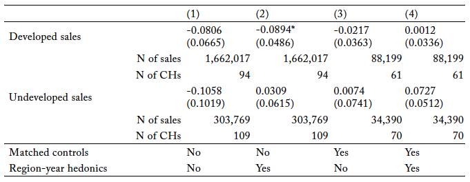
Note: CH = critical habitat. The buffer around CH polygons is 5 km. We used a fuzzy difference-in-differences model for all estimates of the pooled two-way fixed-effects OLS model where the fuzzy period begins at CH proposal and ends at CH finalization. We clustered standard errors at the CH level (parcels that are part of a CH or in that CH’s buffer area form a cluster). Region in this case refers to US Census division. See table S2 for descriptive statistics.

Figure 1. Estimates of the Pooled Two-Way Fixed-Effects OLS Model’s and Panel Model’s Difference-in-Differences Coefficients (± SE x 1.96) across All Critical Habitats (National-Level Analysis)

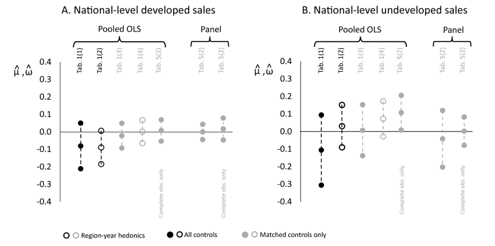
Note: Region in this case refers to US Census Division.

When there are no estimation modifications, national-level estimates of the pooled OLS model support neither of our hypotheses: all else equal, CH treatment did not have a statistically significant impact on developed or undeveloped parcel prices. Alternatively, when we used hedonic functions specific to census division and year instead of the national-level, time-invariant hedonic function, we found that treated developed parcels across the continental United States in ESA-species range space were, on average, 8.6 percent less valuable than they would have been if spared CH treatment.¹⁰ We expected CH to have a positive impact on developed parcel prices. However, estimates of the pooled OLS model at the national level with matched-control sales suggest that CH treatment did not have a statistically significant impact on developed and undeveloped parcel prices, no matter the structure of the hedonic functions. Given that matched controls can mitigate the impact of confounding and omitted variable bias in causal estimates and given that hedonic functions specific to census division and year can capture some of the idiosyncratic real estate market conditions across regions and years, we put the most weight on the results in table 1, column (4).

Plots of the average of $\log \left(V_{j t}\right)$ against treatment timing across all treated and matched-control sales (sales used for the pooled OLS model’s estimates summarized in table 1, columns [3]–[4]) support the conclusion that, at least at the national level, CH treatment had little impact on parcel prices relative to the nearby control sales. As figure 2A indicates, the parallel trend in national-level treated and control developed $\overline{\log \left(V_{j t}\right)}$ before treatment was maintained for six years following treatment. We see a similar pattern for the relative difference between national-level treated and matched-control undeveloped $\overline{\log \left(V_{j t}\right)}$ , both pre- and post-treatment (figure 2B). Parallel trends in the dependent variable prior to treatment are necessary for $\hat{\mu}$ to be considered an unbiased estimator of ATT (Appendix 2).

Across both parcel sale types, national-level treated and matched-control $\overline{\log \left(V_{j t}\right)}$ fell significantly just before CH proposal (indicated by the x-axis value of 0). Recall we do not use any sales that occurred between CH proposal and finalization. Therefore, at $x = 0$ the statistic $\overline{\log \left(V_{j t}\right)}$ is almost entirely made up of sales that occurred just before CH proposal (the CH process, from proposal to finalization, usually takes at least 300 days; therefore, the first post-treatment sale does not typically occur until $x = 1$ ). These dips in $\overline{\log \left(V_{j t}\right)}$ at $x = 0$ could indicate that rumors of an impending CH regulatory process temporarily depress prices in the affected landscape. (The potential for anticipatory effects in the CH process needs to be looked at in future research.) In the end, however, $\overline{\log \left(V_{j t}\right)}$ for both treated and matched-control developed and undeveloped sales quickly rebounded past pretreatment levels after CH establishment.

Figure 2. Mean of Log of Price per ha (Lines Are ±1 SD) by Years before or since Critical-Habitat Establishment

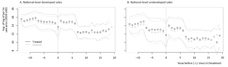
Note: The x-axis gives years before or after treatment, and the y-axis gives the average of $\log \left(V_{j t}\right)$ . Only matched-control sales are included in these averages. A. Treated sales before treatment period: 17,381. Treated sales after treatment period: 13,547. Untreated sales before treatment period: 35,344. Untreated sales after treatment period: 27,355. B. Treated sales before treatment period: 6,351. Treated sales after treatment period: 6,218. Untreated sales before treatment period: 12,534. Untreated sales after treatment period: 13,044.

Estimates of Pooled OLS Model Over Subsets of Critical Habitats Defined by Species or Species Type

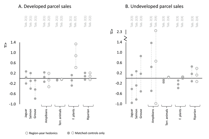
At the individual CH level, we also found little evidence to support our CH-parcel-value hypotheses (table 2, panel A; also see figures S3–S5). The Atlantic-salmon CH process affected developed parcel values in a statistically significant manner, albeit in a direction inconsistent with our hypothesis. Specifically, we found that treated developed parcels in the Atlantic-salmon CH were, on average, 34.9 percent less valuable than they would have been if spared CH treatment (general ESA treatment applies, however).¹¹ However, the other five estimates of the pooled OLS model over sets of parcel sales defined by individual CHs suggest a null treatment effect.

However, we are not sure how much stock to put in the estimates of over sets of sales defined by individual CHs. The plots of $\overline{\log \left(V_{j t}\right)}$ over each of these sets of sales indicate that these DD analyses do not satisfy the pretreatment parallel-trends assumption (figures S6–S8), suggesting that the estimates of the ATT for the individual CHs are biased. Given FWS’s documented efforts to exempt some “developable” vacant parcels from CH regulation that would likely otherwise generate an adverse-modification finding when proposed for development (Fosburgh 2022), we believe the $\hat{\mu}$ ‘s associated with individual CH undeveloped parcel sales are biased upward (Text S2). We are not sure of the direction in bias in the $\hat{\mu}$ associated with individual CH developed parcel sales.

Table 2. Estimates of the Pooled OLS Model’s Difference-in-Differences Coefficient $\hat{\mu}$ across Different Subsets of Critical Habitats Defined by Species or Species Type

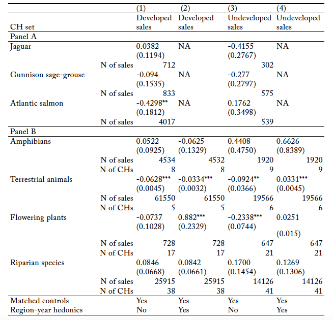
Notes: CH = critical habitat. The buffer around CH polygons is 5 km. We used a fuzzy difference-in-difference model for all estimates of the pooled OLS model where the fuzzy period begins at CH proposal and ends at CH finalization. See table S2 for some descriptive statistics. Panel A: We did not use hedonic functions specific to region and year when estimating model (1) because an individual CH covers just one region. Further, the term $\varphi_{j \in c} \sigma_t$ accounts for any temporal changes in the region’s land-market conditions. Panel B: We clustered standard errors at the CH level (parcels that are part of a CH or in that CH’s buffer area form a cluster). Terrestrial animals are mammals, birds, and reptiles. Riparian species are amphibians, clams, fishes, and snails. Region in this case refers to US counties except in the case of riparian CHs. In the riparian case, region refers to US Census division. The pooled OLS model could not be estimated over riparian-CH treated and control sales with county-year-specific hedonic functions because of rank-order issues. See table S2 for descriptive statistics.

Figure 3. Estimates of the Pooled Two-Way Fixed-Effects OLS Model’s Difference-in-Differences Coefficients (± SE x 1.96) Across Different Subsets of Critical Habitats Defined by Species or Species Type

Note: Region in this case refers to US counties except in the case of riparian critical habitats. In that case, region refers to US Census division.

In contrast to the unexpected $\hat{\mu}$ values across sets of sales defined by individual CHs, estimates of $\mu$ over sales grouped by taxonomy or CH shape type provide some empirical support for our hypothesis that the CH regulation depresses undeveloped parcel values. Specifically, when using one time-invariant hedonic function, treated undeveloped parcels across terrestrial-animal and plant CHs were, on average, 8.8 percent and 20.8 percent less valuable, respectively, than they would have been if spared CH treatment (general ESA treatment applies, however) (table 2, column [3]). Further, in support of our second hypothesis, developed properties in plant CHs did become more valuable relative to their nearby unregulated counterparts when using our preferred hedonic price-modeling technique: hedonic functions specific to region and year.

However, we also found results contrary to our hypotheses. For example, we found that developed parcel sales in terrestrial-animal CHs were 6.1 percent less valuable than they would have been if spared CH treatment (general ESA treatment applies, however) when using one time-invariant hedonic function (table 2, column [1]). Further, evidence that CH regulation depressed undeveloped parcel values disappeared when we used hedonic functions specific to region and year to estimate $\mu$ over sales grouped by taxonomy or CH shape type (table 2, column [4]).

The parallel-pretrend assumption for treated and controlled $\overline{\log \left(V_{j t}\right)}$ appears to hold for the $\hat{\mu}$ ‘s associated with sets of sales defined by amphibian CHs, terrestrial-animal CGs, and riparian species CHs. However, this necessary condition for an unbiased estimate of the ATT does not hold for sales associated with plant CHs (see figures S9–S12). As before, we believe $\hat{\mu}$ ‘s associated with undeveloped parcel sales are biased upward when the parallel-pretrend assumption is not met (Appendix 2).

California-Only Estimates of Pooled OLS Model

When using matched-control sales and a statewide, time-invariant hedonic price function, we found the economic impact of California CH on developed parcel values was consistent with our expectations. Specifically, developed parcels in California CHs and California amphibian CHs only were, on average, 20.4 percent and 14.9 percent more valuable, respectively, than they would have been if spared CH treatment (general ESA treatment applies, however) (table 3, columns [1] and [4]; figure 4). However, given that hedonic functions specific to region and year can capture some of the idiosyncratic real estate market conditions across the state over time, we emphasize the results in columns (3) and (5) of table 3 (matched controls and county-year-specific hedonic functions across all California CHs). Using this preferred model permutation, we found that CH did not have a statistically significant impact on developed parcel prices in California.

The estimated impact of California CH on undeveloped land prices never conformed with our expectations. Across all model permutations, California CH either had no statistically significant effect on undeveloped parcel prices or, contrary to our expectations, positively affected undeveloped parcel price. We found this latter impact when using matched-control sales and a statewide, time-invariant hedonic price function in California amphibian CHs. In this case, undeveloped parcels in California amphibian CHs were, on average, 51.0 percent more expensive than they would have been if spared CH treatment (general ESA treatment applies, however).

Finally, plots of California $\overline{\log \left(V_{j t}\right)}$ —for all CHs and just amphibian CHs—against treatment timing suggest the parallel-trend assumption for unbiased estimates of the ATT in California are met (figures S13–S14).

Table 3. Estimates of the Pooled OLS Model’s Difference-in-Differences Coefficient $\hat{\mu}$ in California Critical Habitat

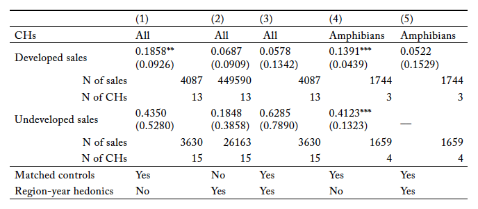
Note: CH = critical habitat. The buffer around CH polygons is 5 km. We used a fuzzy difference-in-differences model for all estimates of the pooled two-way fixed-effects OLS model where the fuzzy period begins at CH proposal and ends at CH finalization. We clustered standard errors at the CH level (parcels that are part of a CH or in that CH’s buffer area form a cluster) in the estimates for columns (1)–(3). Region in this case refers to counties. There are 58 counties in California. Rank-order issues prevented estimation of the difference-in-differences coefficient for California amphibians over undeveloped parcel sales when county-year-specific hedonic functions were used.

Figure 4. Estimates of the Pooled OLS Model’s Difference-in-Differences Coefficients (± SE x 1.96) across All California Critical Habitats

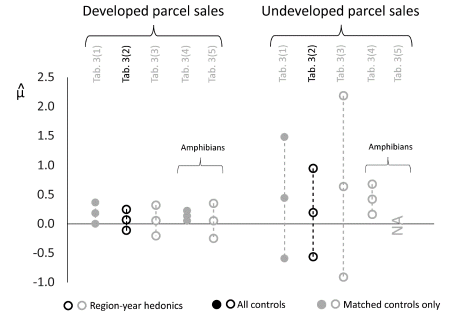
Note: Region in this case refers to counties.

Hedonic-Price-Function Sanity Checks

The pooled OLS is a hedonic price model with DD controls. Therefore, if the signs on $\mathbf{X}_{j t}$ ‘s and $\mathbf{Z}_j$ ‘s estimated coefficients are consistent with the larger hedonic-price-model literature, then we have further evidence that the pooled OLS model is correctly specified. According to past hedonic-price-model research, parcels nearer urban amenities (Ardeshiri et al. 2018), transportation networks (Seo et al. 2014), water (e.g., Dahal et al. 2019), and protected areas (e.g., Kling et al. 2015) are more valuable, all else equal, than parcels further from these landscape features. Further, parcels higher in elevation (e.g., Wu et al. 2004; Sander et al. 2010) but on flat land are more valuable than low-lying land that is sloped (e.g., Ma and Swinton 2012), all else equal. Finally, structures that are larger, have more rooms, have more bathrooms, and are newer are more highly valued than smaller and older structures, all else equal (e.g., Morancho 2003; Sander and Polasky 2009).

Table 4. Fraction of Estimated Hedonic Price Function’s Explanatory Variable Coefficients That Are of Expected Sign in Estimates of Pooled OLS Model across All Critical Habitats (National-Level Estimates), Subsets of Critical Habitats Defined by Species or Species Type, and California Critical Habitats

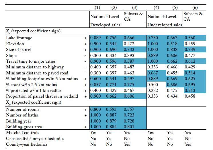
Note: Cells are shaded if more that 50 percent of the coefficient estimates conform to the expected sign. In columns (3) and (6) we include estimated pooled OLS model coefficients from subsets of sales from riparian critical habitats where we used census-division–year hedonics instead of county-year hedonics. The pooled OLS model could not be estimated over riparian-critical-habitat treated and control sales with county-year-specific hedonic functions because of rank-order issues.

In table 4 we indicate the fraction of times an estimated pooled OLS model’s coefficient on a parcel or structural variable had the expected sign. Columns (1) and (4) aggregates all $\mathbf{X}_{j t}$ ‘s and $\mathbf{Z}_j$ ‘s estimated coefficients from the pooled OLS model where we used a single, time-invariant hedonic price function and matched controls (table 1, column [3]; table 2, column [1]; table 3, columns [1] and [4]). Columns (2) and (5) aggregates all $\mathbf{X}_{j t}$ ‘s and $\mathbf{Z}_j$ ‘s estimated coefficients from estimates of the pooled OLS model where we used census-division–year hedonics and matched controls (table 1, column [4]). Finally, columns (3) and (6) pool all $\mathbf{X}_{j t}$ ‘s and $\mathbf{Z}_j$ ‘s estimated coefficients from estimates of the pooled OLS model where we used county-year hedonics and matched controls (table 2, columns [2] and [4]; table 3, columns [3] and [5]).

According to our analysis, the structural variables in vector $\mathbf{X}_{j t}$ very frequently shifted developed parcel prices in ways that aligned with expectations. Further, the land-characteristic variables lake frontage, elevation, parcel size, travel time to nearest major city, nearby building footprint, and proximity to coastline more often than not shifted both developed and undeveloped parcel prices in expected ways. These results suggest that the pooled OLS model is properly specified.

Estimates of Panel Model

In panel A of table 5 we present the panel model’s estimated DD coefficients when using the nationwide panel of sales (a property had to sell at least twice for its sales to be in the data set). The first row in panel B gives $\hat{\omega}$ ‘s when the nationwide panel of sales is limited to those with observations for every variable in $\mathbf{Z}_j$ and, when applicable, $\mathbf{X}_{j t}$ . Finally, the second row in panel B gives $\hat{\mu}$ ‘s from estimates of the pooled OLS model using the nationwide panel of sales with complete observations. Therefore, the DD estimates summarized in panel B, column (1) use the same set of sales; the DD estimates summarized in panel B, column (2) use the same set of sales; etc. (also see figure 1 for plots of $\hat{\omega}$ from table 5, columns [2] and [4]).

Table 5. Estimates of the Panel Model’s Difference-in-Differences Coefficient $\hat{\omega}$ across All Critical Habitats (National-Level Analysis)

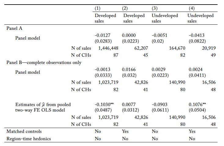
Note: FE = fixed effects. We clustered standard errors at the critical-habitat level (parcels that are part of a critical habitat or in that CH’s buffer area form a cluster). See table S3 for the descriptive statistics.

All estimates of the panel model suggest that CH, at least at the national level, had no statistically significant effect on parcel prices no matter the type of parcel (developed or undeveloped) and control sale type (matched or not) considered. When we compared the estimated DD coefficients from the pooled OLS and panel models using the same set of sales (panel B) holding model permutation constant (same column of Table 5), we found that the panel model was less likely to have found that CH had a statistically significant effect on parcel prices than the pooled OLS model. Therefore, assuming the panel model has a stronger claim to causal interpretation because all time-invariant parcel-level variables, including those that were omitted in the pooled OLS model, are controlled for, we are even more confident in the conclusion that the CH regulation, at least at the national level, has had little impact on parcel values.

Robustness Checks

In our default analysis, control sales are based on a 5 km buffer. We re-estimated model (1) at the national level and across the various CH subsets using buffer sizes of 3 and 10 km. We found that buffer size did not affect national-level estimates of model (1) (table S4 and figure S15). However, alternative buffer sizes did change the statistical significance of $\hat{\mu}$ for several CH subsets (table S5 and figure S16). Overall, however, we see no evidence of systematic change in $\hat{\mu}$ as we change buffer size. For example, the number of statistically significant $\hat{\mu}$ ‘s did not increase or decrease in buffer size. Nor did the magnitudes of the various $\hat{\mu}$ ‘s shift in a consistent manner as we changed buffer size. The sensitivity of some model results generated over subsets of sales grouped by CH taxonomy or CH shape type to buffer-size choice reinforces our topline conclusion that the impact of CH on land prices cannot be reduced to a simple, consistent narrative.

Recent econometric literature has discussed the possibility of biased DD estimators when treatment timing is staggered (Goodman-Bacon 2018; de Chaisemartin and d’Haultfoeuille 2020; Text S2). Staggered-treatment bias cannot be an issue in our individual-species CH estimates (table 2, panel A) but is a potential problem in all other model estimates. Per Callaway and Sant’Anna (2019), we eliminate the potential of bias in the pooled OLS model’s DD estimator due to staggered treatment by estimating the model over a cohort of CHs that were proposed and finalized at approximately the same time (tables S6–S8; figure S17). To further reduce the potential impact of unobserved policy changes affecting parcel prices in these CHs and their relevant controls, we only included treated sales and relevant matched-control sales that occurred within two years of treatment (pretreatment sales are not limited by time). Again, we found these results largely failed to confirm our hypotheses. These results suggest that the inconsistent impact of CH on parcel values we found when using the pooled OLS model cannot be blamed on staggered-treatment bias.

Some parcels flagged as developed in our database (zoned as rural-residential with positive building footprint) are likely to be viewed by developers as still “developable.” For example, consider a rural-residential 80-acre parcel with one house on it. We consider this parcel “developed” given that it has a nonzero building footprint. Suppose the conversion of the parcel to a subdivision would generate millions of dollars in net revenues for a developer. In this case, the “developed” parcel would be very attractive to a developer, as the cost of removing the one house would be negligible compared to the value of the parcel after subdivision. Therefore, we experimented with dividing our developed parcels into two types: those that we believe could generally be redeveloped at little relative cost (like the fictitious 80-acre parcel described above) and those that we believe would be much costlier or more impractical to redevelop. We assume this latter category would for the most part be made up of developed parcels where the new owners would use the parcel as is or implement marginal changes at most.

We believe a parcel’s building-to-parcel-area ratio (BPR) provides the best means of separating developed parcels into these two types. We assume developed parcels with a low BPR—lower than 0.063 across all parcels categorized as “rural residential”—were like our fictitious 80-acre parcel with one house: very developable (0.063 is at the 90th percentile of the BPR-ratio distribution across all “rural residential” parcels in our data set). On the other hand, we assumed parcels with BPRs greater than 0.063 were much less likely to be bought for redevelopment. We found that the developed parcels with a high BPR have an estimated pooled OLS DD coefficient similar in magnitude to the estimated DD coefficient associated with the entire pool of developed parcels (table 1, column [3]), albeit both estimated coefficients are not statistically significant (table S9). We also found that developed parcels with a low BPR have an estimated pooled OLS DD coefficient similar in magnitude to the estimated DD coefficient associated with undeveloped parcels (table 1, column [3]), albeit both estimated coefficients are not statistically significant. Overall, the subdivision of developed parcels into two sets based on building footprint does not change our assessment of national-level results.

6. Conclusion

We found that CH treatment infrequently had a statistically significant impact on parcel values. Further, when a DD coefficient was statistically significant, the impact was often at odds with the hypothesized direction. Finally, the scale of analysis affected our findings. National-level analyses indicated little to no effect of the CH regulation on parcel values, while some more focused analyses (e.g., California amphibian CHs only or terrestrial-animal CHs only) did find some regulatory effect on parcel prices. Therefore, the impact of CH on parcel prices cannot be reduced to a simple, consistent narrative. Determining why some CHs create positive economic impacts, why others create negative economic impacts, and why others have no apparent economic impact at all are the questions that future CH economic research must answer.

There are multiple potential reasons why we found regulatory impacts that are at odds with previous findings. First, across all treated and matched-control sales, 95.4 percent of developed and 95.3 percent of undeveloped parcel sales we analyzed were not from California. Almost all other previous CH impact analyses have focused on California. For example, the DD analysis in Auffhammer et al. (2020) used just two CHs in California. Second, we used a comprehensive, consistent, and national-level data set of observed parcel sales, ZTRAX, that has never been used in CH analyses before. Third, we emphasized the DD results we obtained with a matched-control set. Only a few of the previous CH impact analyses used matched (or synthetic) controls, an approach that many researchers have found improves causal identification. Fourth, we measured the impact of the CH regulation on parcel prices, not the impact of a mixture of CH and broader ESA regulations on land prices, by ensuring that every parcel sale in our data set, treated or control, occurred when the parcel was in the geographic range of at least one listed species. We are not sure how careful previous studies of CH economic impact were at separating these regulatory impacts.

Several reasons could explain why undeveloped land prices are, for the most part, not affected by CH in expected ways. The most obvious explanation is that the CH regulation, especially when separated from the broader ESA regulation, does not have much regulatory bite. First, many development projects in many CH areas may not require federal permits or use federal moneys, thereby never requiring CH consultation. Second, even in cases where the federal nexus applies, it could be that required changes or activity delays are most often minor, creating little effect on prices. In fact, past FWS administrators have claimed that the CH regulation is superfluous given the broader ESA regulations.¹² If this sentiment guides the FWS in its application of CH regulations, then it would not be surprising to find that the CH regulation in and of itself has little economic impact.

Alternatively, undeveloped parcel prices could have fallen less than expected in CH areas because of local land-supply effects. For example, suppose some undeveloped parcels in a CH area became “undevelopable” due to CH regulations. Further, suppose the remaining undeveloped parcels in the CH can be developed at little additional cost or delay. In this case, the total supply of “developable” land has fallen across the CH and its 5 km buffer—thereby keeping local undeveloped parcel prices elevated—but the difference in development cost between treated (but “developable”) and control undeveloped parcels is minor. The temporal pattern of average undeveloped parcel prices pre- and post-treatment in figure 1B comport with this story: notice that for five years after CH establishment, both treated and control average undeveloped parcel prices are elevated relative to their average prices before treatment.

There are other mechanisms that may keep undeveloped land prices in CH areas higher than expected. For example, housing developers may be willing to put up with the hassle and uncertainty of developing land in CH areas if they believe that homeowners will be willing to pay a premium for houses in these regulated areas. In addition, undeveloped land prices in some CH areas could be higher than expected because of competition from conservation organizations. If CH designation triggers conservation organizations’ attempts to buy undeveloped land in a CH for biodiversity conservation, then the higher demand for undeveloped land in the CH could maintain prices despite the additional regulatory scrutiny of private development activities in the same area (Armsworth et al. 2006).

The conclusion that the CH regulation does not have much actual regulatory bite could also explain why we did not consistently find higher developed parcel prices in CH areas after treatment. For example, if CH does little to prevent development, then open spaces adjacent to homes in CH areas are just as susceptible to development as open spaces adjacent to homes in nearby, non-CH areas. If this is true, then homes in CH areas would not command a premium relative to homes in nonregulated areas. Finally, homebuyers might view homes right outside a CH area—in the buffer—as equivalent to homes inside a CH area, all else equal. Assuming CH does make the preservation of open space more likely, homes in the buffer will be near unique open spaces. For many homeowners, being near unique open spaces could be just as valuable as being within unique open spaces.

To summarize, when using land prices as a metric of regulatory impact, the CH regulation has inconsistent and often nonexistent impacts. The CH regulation is a biodiversity-protection program that—when evaluated separately from the larger ESA regulation that it is part of—only sporadically creates the costs that theory suggests it is capable of generating. Therefore, we wonder whether the program creates much biodiversity protection at all. We assume that an effective biodiversity-protection program would consistently generate observable costs; we are skeptical of the efficacy of a program that appears to cost little.

Of course, the CH regulation could consistently create economic costs despite our claims to the contrary. We already noted that our DD estimators are unbiased estimators of the ATT if and only if various data and modeling assumptions hold (Appendix 2). However, even if all of these data and modeling assumptions hold, there are other reasons to suspect that the DD estimators generated by our models are biased. Further, there are some data problems that we cannot solve at this time. We detail some of the other potential sources of DD estimator bias and data issues below to be as transparent as possible. Future research on the economic impact of CH would be more precise if it corrected the problems we identify below. However, despite these caveats, the general statistical insignificance of the estimated DD coefficients and the consistent inconsistency in our results means we are confident in our assessment that, while the impact of CH on land prices cannot be reduced to a simple, consistent narrative, the CH regulation above and beyond other ESA regulations does not generate significant economic impacts.

We have hypothesized that the consultation requirement and the possibility of a “destruction or adverse modification finding” dampens developer demand for undeveloped land in the CH, all else equal, and accordingly should dampen prices for those lands, all else equal. However, a more nuanced model of CH’s impact on undeveloped parcel values would surmise that only some developable parcels would be likely to require the developer to “implement reasonable and prudent alternatives to avoid destruction or adverse modification of critical habitat,” and therefore only these parcels would have dampened prices. Therefore, a critical unobserved variable in our analysis of undeveloped parcel prices in CH areas is $M_{j t}$ , parcel j’s probability of a destruction or adverse-modification finding if considered for development. And even though using matched-control sales can reduce the potential of omitted variable bias, it may not completely eliminate it. See Appendix 3 for a detailed discussion on the bias that an omission of $M_{j t}$ could engender in the undeveloped-parcel DD estimator.

Selection bias also likely affects our DD coefficient estimates. CHs that have been revised several times (“complex” CHs) due to new information, new scientific data, political pressure, or court cases are not included in our study because they make identification of the economic impact of CH more difficult (i.e., certain parcels may pop in and out of CH rapidly). However, we suspect that these complex CHs are likely to have had a greater impact on land prices than the “simple” CHs that we currently include in our study (e.g., see Klick and Ruhl 2020). Presumably, their imposition of high economic cost is one of the main reasons for “complex” CHs’ unsettled path to finalization (see Appendix 4).¹³ Therefore, since we do not include the potentially more expensive CHs, our estimates of the DD coefficients $\mu$ and $\omega$ likely underestimate the actual penalty that CH imposes on American land values.

In addition, there are several data issues that hamper our ability to precisely identify the impact of CH on parcel prices. First, even though we claim that “simple” CHs have consistent boundaries between the proposal and finalization stages, that is not always the case. Minor changes can be made between these two stages. For example, in the FR that announces the final designation of CH for Gunnison sage-grouse, the section stating that “we modified the boundaries of this critical habitat designation around the City of Gunnison” refers to boundaries set forth in the proposed CH (USDOIFWS 2013; 2014). We use fuzzy DD timing in order to avoid having to account for sales that took place on land proposed for CH that may not be in the final CH; in our model, either a parcel was certainly regulated by CH or it was not. However, market participants may not realize that land proposed for regulation was not finalized as CH. Therefore, there may be some post-CH-establishment control sales in our model estimates that were affected by the perception of CH regulation.

Second, during the course of our research we learned that some of the digital maps of CH areas available from the FWS’s website only approximate the actual CH areas (Maura Flight, pers. comm., June 25, 2021). Official CH areas are described with coordinates and printed maps in FR notices, and, in some cases, the digital representation of these areas does not exactly follow official boundaries. Therefore, our analysis likely has some false positives (parcels that we treat as “treated” but in fact were not) and false negatives (parcels that we treat as “not treated” but in fact were). We will investigate the impact of digital map measurement error in future iterations of this research.

A third identification problem is created by the perceived versus actual regulatory “bite” of the CH regulation. As we argued above, our findings suggest that the CH regulation adds little regulatory bite above and beyond more general ESA regulations. This conclusion may be particularly germane in CH areas that include occupied habitat. The destruction or modification of occupied habitat is already prevented by ESA regulations; in these areas CH regulations are superfluous. However, CH can also cover unoccupied habitat. In these areas the CH regulation may be impactful because the take and jeopardy provisions of the ESA are less relevant in these landscapes (Maura Flight, pers. comm., June 25, 2021). In unoccupied habitat areas, the CH regulation may be the only relevant barrier to habitat destruction or modification. Therefore, the better DD model for investigating the impact of CH on land values may be to treat CH areas that include unoccupied habitat as treated areas and all other ESA-affected areas, including CH area over occupied habitat, as the control areas.

We believe that many of these data problems could be resolved if the FWS tweaked the data it makes available to the public. First, the FWS should publish digital maps of every proposed CH, every proposed revision, and every final CH, not just the latest final CH. Second, each published CH map should specify known habitat areas, occupied habitat, and unoccupied habitat. Third, the FR notices that describe and codify the CH-making process need to become more consistent in the data they present and the layout of the data. Tables that indicate the breakdown of proposed and final CH areas by land tenure (private, local government, tribal, etc.) need to be in every FR notice. Further, if there has been a change in the area by land tenure from an earlier FR notice, the specific reason and not a vague reference to one of the ESA regulations should be noted. For example, a specific statement would read, “Thirty hectares of private forest in the previous CH proposal were removed in the current proposal because Weyerhaeuser has agreed to place thirty hectares of land they own in a Habitat Conservation Plan.”

Acknowledgments

The authors acknowledge the Minnesota Supercomputing Institute at the University of Minnesota for providing resources that contributed to the research results reported within this paper. We thank Zillow for having made ZTRAX available free of charge for US academic, nonprofit, and governmental researchers. Christoph Nolte acknowledges support from the Department of Earth and Environment at Boston University, the Junior Faculty Fellows program of Boston University’s Hariri Institute for Computing and Computational Science, and the Nature Conservancy. The authors also acknowledge the insights provided by Katherine Fosburgh, Maura Flight, Robert W. Paterson, and the participants in the 2021 PLACES webinar.

References

Angrist, J., and J.-S. Pischke. 2009. Mostly Harmless Econometrics. Princeton, NJ: Princeton University Press.

Ardeshiri, Ali, Ken Willis, and Mahyar Ardeshiri. 2018. “Exploring Preference Homogeneity and Heterogeneity for Proximity to Urban Public Services.” Cities 81: 190–202. https://doi.org/10.1016/j.cities.2018.04.008.

Armstrong, A. 2002. “Critical Habitat Designations under the Endangered Species Act: Giving Meaning to the Requirements for Habitat Protection.” South Carolina Environmental Law Journal 10: 53.

Armsworth, Paul R., Gretchen C. Daily, Peter Kareiva, and James N. Sanchirico. 2006. “Land Market Feedbacks Can Undermine Biodiversity Conservation.” PNAS 103 (14): 5403–8. https://doi.org/10.1073/pnas.0505278103.

Auffhammer, Maximilian, Maya Duru, Edward Rubin, and David L. Sunding. 2020. “The Economic Impact of Critical-Habitat Designation: Evidence from Vacant-Land Transactions.” Land Economics 96 (2): 188–206. https://doi.org/10.3368/le.96.2.188.

Black, Katie Jo. 2018. “Wide Open Spaces: Estimating the Willingness to Pay for Adjacent Preserved Open Space.” Regional Science and Urban Economics 71: 110–21. https://doi.org/10.1016/j.regsciurbeco.2018.06.001.

Bošković, Branko, and Linda Nøstbakken. 2017. “The Cost of Endangered Species Protection: Evidence from Auctions for Natural Resources.” Journal of Environmental Economics and Management 81: 174–92.

Callaway, Brantly, and Pedro H. C. Sant’Anna. 2019. “Difference-in-Differences with Multiple Time Periods.” http://dx.doi.org/10.2139/ssrn.3148250.

De Chaisemartin, C., and X. d’Haultfoeuille. 2020. “Two-Way Fixed Effects Estimators with Heterogeneous Treatment Effects.” American Economic Review 110 (9): 2964–96.

Colorado Natural Heritage Program. 2019. The Colorado Ownership, Management and Protection Map (COMaP). https://comap.cnhp.colostate.edu.

Cunningham, Scott. 2020. Causal Inference. The Mixtape. New Haven, CT: Yale University Press.

Dahal, Ram P., Robert K. Grala, Jason S. Gordon, Ian A. Munn, Daniel R. Petrolia, and J. Reid Cummings. 2019. “A Hedonic Pricing Method to Estimate the Value of Waterfronts in the Gulf of Mexico.” Urban Forestry & Urban Greening 41: 185–94. https://doi.org/10.1016/j.ufug.2019.04.004.

Daw, J. R., and L. A. Hatfield. 2018. “Matching and Regression to the Mean in Difference-in-Differences Analysis.” Health Services Research 53 (6): 4138–56. https://doi.org/10.1111/1475-6773.12993.

ESRI. 2009. North America Water Polygons. https://hub.arcgis.com/datasets/esri::usa-detailed-water-bodies/explore?location=31.308641%2C-113.614487%2C4.59.

Fois, M., G. Fenu, and G. Bacchetta. 2019. “Estimating Land Market Values from Real Estate Offers: A Replicable Method in Support of Biodiversity Conservation Strategies.” Ambio 48: 313–23. https://doi.org/10.1007/s13280-018-1074-3.

Garibaldi, L. A., F. J. Oddi, F. E. Miguez, et al. 2021. “Working Landscapes Need at Least 20% Native habitat.” Conservation Letters 14 (2): e12773. https://doi.org/10.1111/conl.12773.

Geoghegan, Jacqueline. 2002. “The Value of Open Spaces in Residential Land Use.” Land Use Policy 19 (1): 91–98. https://doi.org/10.1016/S0264-8377(01)00040-0.

Goodman-Bacon, Andrew. 2018. “Difference-in-Differences with Variation in Treatment Timing.” NBER Working Paper No. 25018, National Bureau of Economic Research, Cambridge, MA, September.

Hanley, Nick, Simanti Banerjee, Gareth D. Lennox, Paul R. Armsworth. 2012. “How Should We Incentivize Private Landowners to ‘Produce’ More Biodiversity?” Oxford Review of Economic Policy 28 (1): 93–113. https://doi.org/10.1093/oxrep/grs002.

Harvard Forest. 2020. New England Protected Open Space.

Homer, C., J. Dewitz, L. Yang, S. Jin, P. Danielson, G. Xian, J. Coulston, N. Herold, J. Wickham, and K. Megown. 2015. “Completion of the 2011 National Land Cover Database for the Conterminous United States—Representing a Decade of Land Cover Change Information.” Photogramm. Eng. Remote Sensing 81: 345–54.

Kiel, K. 2005. “Environmental Regulations and the Housing Market: A Review of the Literature.” Cityscape 8 (1): 187–207. https://www.jstor.org/stable/20868574.

Klick, Jonathan, and J. B. Ruhl. 2020. “The Costs of Critical Habitat or Owl’s Well That Ends Well.” Faculty Scholarship at Penn Law 2231. https://scholarship.law.upenn.edu/faculty_scholarship/2231.

Kling, R.W., T. S. Findley, E. Gahramanov, et al. 2015. “Hedonic Valuation of Land Protection Methods: Implications for Cluster Development.” Journal of Economics and Finance 39: 782–806. https://doi.org/10.1007/s12197-014-9279-1.

Kolstad, Charles D., and Frances C. Moore. 2020. “Estimating the Economic Impacts of Climate Change Using Weather Observations.” Review of Environmental Economics and Policy 14 (1): 1–24.

Kremen, Claire, and Adina M. Merenlender. 2018. “Landscapes That Work for Biodiversity and People.” Science 362 (6412): eaau6020.

List, J. A., M. Margolis, and D. E. Osgood. 2006. “Is the Endangered Species Act Endangering Species?” NBER Working Paper No. 12777, National Bureau of Economic Research, Cambridge, MA.

Ma, S., and S. M. Swinton. 2012. “Hedonic Valuation of Farmland Using Sale Prices versus Appraised Values.” Land Economics 88 (1): 1–15.

Melstrom, R. T. 2021. “The Effect of Land Use Restrictions Protecting Endangered Species on Agricultural Land Values.” American Journal of Agricultural Economics 103: 162–84. https://doi.org/10.1111/ajae.12127.

Microsoft. 2018. US Building Footprints. Accessed February 2, 2020. https://github.com/microsoft/USBuildingFootprints.

Morancho, Aurelia Bengochea. 2003. “A Hedonic Valuation of Urban Green Areas.” Landscape and Urban Planning 66 (1): 35–41.

Nelson, A. 2008. Travel Time to Major Cities: A Global Map of Accessibility. Global Environment Monitoring Unit, Joint Research Centre of the European Commission, Ispra, Italy. http://forobs.jrc.ec.europa.eu/products/gam/sources.php.

Nolte, C. 2020. “High-Resolution Land Value Maps Reveal Underestimation of Conservation Costs in the United States.” Proceedings of the National Academy of Science 117: 29577–29583.

Nolte, C., K. Boyle, A. Chaudhry , C. Clapp, D. Guignet, H. Hennighausen, I. Kushner, Y. Liao. 2021. “Studying the Impacts of Environmental Amenities and Hazards with Nationwide Property Data: Best Data Practices for Interpretable and Reproducible Analyses.” Available from SSRN: https://papers.ssrn.com/sol3/papers.cfm?abstract_id=3900806.

Quigley, John M., and Aaron M. Swoboda. 2007. “The Urban Impacts of the Endangered Species Act: A General Equilibrium Analysis.” Journal of Urban Economics 61 (2): 299–318.

Sander, Heather, Stephen Polasky, and Robert G. Haight. 2010. “The Value of Urban Tree Cover: A Hedonic Property Price Model in Ramsey and Dakota Counties, Minnesota, USA.” Ecological Economics 69 (8): 1646–56.

Sander, H. A., and S. Polasky. 2009. “The Value of Views and Open Space: Estimates from a Hedonic Pricing Model for Ramsey County, Minnesota, USA.” Land Use Policy 26 (3): 837–45.

Seo, Kihwan, Aaron Golub, and Michael Kuby. 2014. “Combined Impacts of Highways and Light Rail Transit on Residential Property Values: A Spatial Hedonic Price Model for Phoenix, Arizona.” Journal of Transport Geography 41: 53–62. https://doi.org/10.1016/j.jtrangeo.2014.08.003.

Sunding, David L. 2003. “Economic Impacts of Critical Habitat Designation for the Coastal California Gnatcatcher.” California Resource Management Institute Working Paper, California Resource Management Institute.

Sunding, D., A. Swoboda, and D. Zilberman. 2003. “The Economic Costs of Critical Habitat Designation: Framework and Application to the Case of California Vernal Pools.” California Resource Management Institute.

Trust for Public Land & Ducks Unlimited. 2020. The National Conservation Easement Database https://www.conservationeasement.us/.

US Census Bureau (USCB). 2019. 2019 TIGER/Line Shapefiles. https://www.census.gov/cgi-bin/geo/shapefiles/index.php.

US Department of the Interior. US Fish and Wildlife Service (USDOIFWS). 2000. Endangered and Threatened Wildlife and Plants; Proposed Determination of Critical Habitat for the Peninsular Bighorn Sheep. Proposed rule. 65 Federal Register 129 (July 5).

US Department of the Interior. US Fish and Wildlife Service (USDOIFWS). 2001. Endangered and Threatened Wildlife and Plants; Final Determination of Critical Habitat for Peninsular Bighorn Sheep. Final rule. 66 Federal Register 22 (February 1).

US Department of the Interior. US Fish and Wildlife Service (USDOIFWS). 2005. Endangered and Threatened Wildlife and Plants; Designation of Critical Habitat for the Pacific Coast Population of the Western Snowy Plover. Final rule. 70 Federal Register 188 (September 29).

US Department of the Interior. US Fish and Wildlife Service (USDOIFWS). 2008. Endangered and Threatened Wildlife and Plants; Designation of Critical Habitat for the Peninsular Ranges Population of Desert Bighorn Sheep (Ovis canadensis nelsoni). Proposed rule. 73 Federal Register 166 (August 26).

US Department of the Interior. US Fish and Wildlife Service (USDOIFWS). 2009. Endangered and Threatened Wildlife and Plants; Designation of Critical Habitat for Peninsular Bighorn Sheep and Determination of a Distinct Population Segment of Desert Bighorn Sheep. Final rule. 74 Federal Register 70 (April 14).

US Department of the Interior. US Fish and Wildlife Service (USDOIFWS). 2013. Endangered and Threatened Wildlife and Plants; Designation of Critical Habitat for Gunnison Sage-Grouse. Proposed Rule. 78 Federal Register 8 (January 11).

US Department of the Interior. US Fish and Wildlife Service (USDOIFWS). 2014. Endangered and Threatened Wildlife and Plants; Designation of Critical Habitat for Gunnison Sage-Grouse. Final rule. 79 Federal Register 224 (November 20).

US Fish and Wildlife Service (USFWS). 2017. Critical Habitat. What Is It? https://www.fws.gov/endangered/esa-library/pdf/critical_habitat.pdf.

US Fish and Wildlife Service. (USFWS). 2018. National Wetlands Inventory: Seamless Wetlands Data. https://www.fws.gov/wetlands/data/data-download.html.

US Fish and Wildlife Service. (USFWS). CRITHAB_POLY and CRITHAB_LINE zip files. Accessed March 27, 2020. https://ecos.fws.gov/ecp/report/table/critical-habitat.html.

US Fish and Wildlife Service (USFWS). 2021. USFWS Refined Range Maps for Threatened and Endangered Species. Accessed February 19, 2021. http://www.ecos.fws.gov.

US Geological Survey (USGS) 2017a. National Elevation Dataset. https://lta.cr.usgs.gov/NED.

US Geological Survey. (USGS) 2017b. National Hydrography Dataset (NHD) USGS National Map. https://nhd.usgs.gov/NHD_High_Resolution.html.

US Geological Survey (USGS). 2018. Protected Areas Database of the United States (PAD-US).

Wallace, James E. 1995. “Financing Affordable Housing in the United States.” Housing Policy Debate 6 (4): 785–814.

Wu, J., R. M. Adams, and A. J. Plantinga. 2004. “Amenities in an Urban Equilibrium Model: Residential Development in Portland, Oregon.” Land Economics 80 (1): 19–32.

Yagerman, Katherine Simmons. 1990. “Protecting Critical Habitat under the Federal Endangered Species Act.” Environmental Law 20 (4): 811.

Zabel, J. E., Paterson, R., 2006. “The Effects of Critical Habitat Designation on Housing Supply: An Analysis of California Housing Construction Activity.” Journal of Regional Science 46 (1): 67–95.

Zillow. 2019. ZTRAX: Zillow Transaction and Assessor Dataset, 2019-Q4. http://www.zillow.com/ztrax.

Estimating the Impact of Critical-Habitat Designation on the Values of Developed and Undeveloped Parcels

Executive Summary

Resources

Focuses

Federal Agencies

1. Introduction

2. Previous Literature on the Critical Habitat Regulation’s Economic Impact

3. Data