Down Payments and the Homeownership Dream: Not Such a Barrier After All?

Hedlund, Aaron

Introduction

For decades, America’s collective psyche has equated the promise of upward mobility and economic opportunity with the dream of owning a house. Also, in the policy arena, the United States has experimented with untold number of programs to encourage homeownership. These policies include the tax deductibility of mortgage interest, the lack of taxation of imputed rents, government-sponsored enterprises to increase liquidity in the secondary mortgage market, and billions in spending on down payment assistance and other direct aid. In all, these explicit and implicit costs amount to hundreds of billions of dollars per year for the government.¹

Looking beyond legislative action, capital markets have also undergone significant changes in a way that has dramatically altered the landscape for housing finance. Of particular importance, the past twenty years have witnessed the arrival of many new mortgage instruments, often featuring extremely low down payments. Despite these innovations, the left panel of figure 1 projects the image of a mostly stable aggregate homeownership rate over the past half century. The episode most worth mentioning that does, in fact, demonstrate sizable homeownership movements is the post-1998 housing boom and bust that coincided with a period of historically low interest rates. The right panel shows that down payments were also quite low during the boom, and the FHFA reports that the share of new loans with greater than 90 percent leverage rose from less than 1-in-10 in the late 1980s to 1-in-4 a decade later.

Figure 1. (Left) Homeownership Rates by Age; (Right) Median Down Payment Percentage

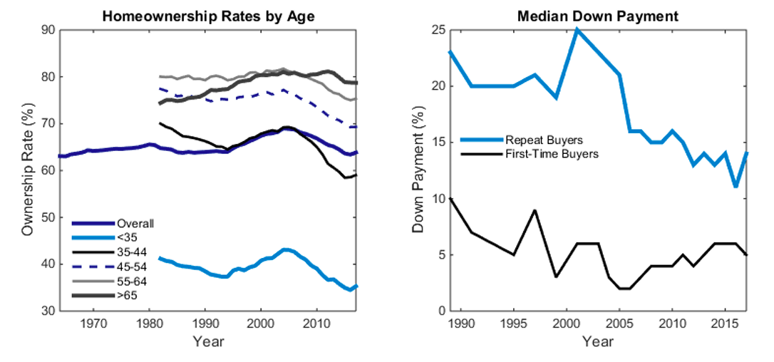Source: (Left) US Census Data; (Right) National Association of Realtors

In the post-housing crash environment of today, many policymakers interested in minimizing the chance of a repeat episode now confront the fear that any efforts to reduce leverage might have a deleterious impact on homeownership. Putting aside any ongoing debates over the desirability of homeownership as a policy goal in the first place, the aim of this paper is to test whether such a fear is warranted.² Specifically, the central question in this paper is whether and under what conditions loose borrowing limits are required for a high homeownership rate to prevail. The main finding is that, subject to a few caveats, long-run homeownership is not very sensitive to down payment requirements. As one might expect, homeownership does decline initially after an unexpected tightening in down payment requirements, but over time it tends to gradually revert to its original level.

These conclusions emerge from a structural macroeconomic model with heterogeneity and incomplete markets, portfolio choice, and a rich credit market that features long-term mortgage contracts and the possibility of foreclosures in equilibrium. Households face the decision to rent apartment space each period or purchase a house, which they can finance using a combination of accumulated savings and mortgage debt. Even without aggregate shocks, uninsurable income risk generates constant churn between renting and owning that is affected by the presence of credit constraints. The main experiments then subject the stationary economy to differing magnitudes of a permanent, unexpected tightening of the down payment constraint applicable at origination under a variety of specifications.

In the benchmark calibration, which features a non-binding 125 percent loan-to-value cap at origination and a utility function with housing and consumption as complements, homeownership falls by 2.4 percentage points in the initial aftermath of imposing a 20 percent down payment requirement. Most of this decline comes from a depressed flow of renters into homeownership rather than an exodus of homeowners into renting. During this period of declining homeownership, however, renters begin accumulating assets, which sows the seeds for a long-run homeownership recovery. Strikingly, even imposing a 50 percent minimum down payment results in no perceptible change to the long-run homeownership rate, although the transition path exhibits a stark and protracted adjustment phase.

In the long run, little changes qualitatively for the 20 percent down payment case if the model is recalibrated with Cobb-Douglas preferences that create greater substitutability between housing and consumption. Instead of not budging at all, the long-run homeownership rate is reduced by 2.6 percentage points, which is quite modest given that nearly one-fifth of outstanding loans and over 85 percent of originations for new purchases are at above 80 percent leverage prior to the tightening. However, beneath this long-run stability, patterns emerge from the short-run dynamics that highlight the role of substitutability. With complements, homeownership and consumption recover in tandem, whereas with substitutes, consumption recovers much more quickly at the expense of housing.

These results align well with the relative stability in the homeownership rate over the past 50 years. However, the post-1998 boom and bust in homeownership bears examination. According to the model, homeownership does respond in the long run to changes in interest rates. Thus, the homeownership boom from 64 percent to 69 percent can be viewed as the combination of a temporary response to looser down payment requirements and a permanent response to lower interest rates. The subsequent decline is likely attributable at least in part to the upheaval in credit markets and the regulatory regime from the financial crisis.

When it comes to prices, a key trade-off emerges: the greater the adjustment in prices, the smaller the movement in quantities—namely, homeownership. In the extreme case of a fixed total housing stock, introducing a 20 percent down payment requirement switches out the short-run homeownership decline from before with an 8 percent temporary fall in house prices. However, just as with homeownership, house prices exhibit long-run mean reversion for both preference specifications.

Lastly, to further test robustness, the quantitative experiments are repeated with a re-calibrated model with life cycle features. In a setting where new households start life as renters with low income and zero assets (i.e., there are no bequests, inter vivos transfers, or intergenerational persistence in earnings), the homeownership rate exhibits a more exaggerated short-run response to tighter down payments but, again, very little long-run change. The model reveals that, while the homeownership rate does fall for young households—for the simple reason that they take longer to accumulate assets for a down payment—it increases for older households. This finding can be explained by the fact that, while the rent-to-own rate falls, the own-to-rent rate acts as a counterbalance by falling as well. Homeowners anticipate that, if they were to ever become renters, the higher down payment barrier slows any possible future transition back into homeownership. Homeowners are therefore more reluctant to switch from owning to renting in the first place.

The central takeaway from these findings is that the homeownership rate does not exhibit any significant long-run relationship with the size of minimum down payments. One practical implication is that policymakers interested in promoting homeownership should expand their horizons beyond the subsidization of high leverage mortgages to consider alternatives that do not risk exacerbating macroeconomic fragility. Investigating these options is beyond the scope of this paper, but one lesson which emerges is that reducing the costs of ownership is likely to be more effective than encouraging people to take out risky loans early in life.

Relationship to the Literature

This paper is related to several different strands of economic literature. On the empirical side, many papers have examined the relationship between down payment requirements and homeownership. Acolin et al. (2017) provide a good summary of this literature and also present their own findings from 2010 to 2013 that being borrowing constrained significantly reduces the probability of an individual owning a house. Haurin, Hendershott, and Wachter (1997) come to a similar conclusion for the period from 1985 to 1990. At a more aggregated level, Chiuri and Jappelli (2003) show that countries with higher down payment ratios have lower homeownership, even after various controls. More recently, Anenberg et al. (2017) construct a richer measure of mortgage credit availability across the credit score distribution, and they exploit geographical variation to demonstrate that borrowing constraints played an important role during the recent housing cycle.

The aforementioned empirical findings are compatible with the implications of the structural model in this paper. At any given point in time, a tightening in down payment requirements shuts out constrained households from the owner-occupied market. However, the important lesson that emerges from the model is that asset accumulation gradually reverses the initial aggregate homeownership decline. Engelhardt (1996) validates this channel empirically by demonstrating how constrained households depress consumption to build savings for a down payment.

This paper also contributes to the structural literature. On the more theoretical side, Ortalo-Magné and Rady (1999, 2006) show the importance of credit constraints for homeownership, prices, and the housing ladder. In addition, Gete and Reher (2016) develop a two-period, heterogeneous agents model featuring housing tenure choice to study optimal loan-to-value regulation. Most related on the quantitative side, Chambers, Garriga, and Schlagenhauf (2009) study the interplay between homeownership and the mortgage market. They find that the introduction of new loan products explains most of the rise in homeownership between 1994 and 2005. Like this paper, they also show that evolving down payments do not produce a permanent change in homeownership, but for far different reasons. In their framework, all homeowners who take out a fixed-rate mortgage are compelled to make the same down payment. By contrast, the model in this paper includes both an extensive and intensive margin for borrowing and matches the distribution of leverage. Their closed economy and uniform borrowing assumptions imply that a loosening in down payments necessarily increases the demand for borrowing. As a result, interest rates rise and suppress homeownership. The mechanism in this paper has nothing to do with general equilibrium interest rates but instead involves asset accumulation dynamics that are impacted by the degree of intratemporal substitution. In recent work, Li et al. (2016) also establish the importance of such substitution between housing and consumption for explaining housing dynamics.

Empirically, Gete and Zecchetto (2018) exploit heterogeneity across MSAs in lenders’ regulatory exposure to the Dodd-Frank Act to test for the effects of tighter credit on rent growth following the housing crisis. They find that each 1 percentage point increase in loan denial rates fuels 1.3 percent higher rent growth primarily through a shift in housing tenure from ownership to renting. Their analysis is consistent with the finding in this paper of a short-run link between credit constraints and homeownership, but critically, the relationship attenuates over time. Also recently, Grundl and Kim (2018) use property-level data to assess the impact of changes in conforming loan limits on homeownership. They find no robust effect and conclude that mortgage guarantees could be significantly reduced without harming homeownership, which is in keeping with the results of this paper.

A Simple Model

Households with income $e$ enjoy consumption $c$ , shelter $s$ , and terminal wealth $y$ ,

(1) $\begin{equation*} U(c,s,y) = \omega ln(c) + (1 - \omega)ln(s) + \phi ln(y). \end{equation*}$

Households can obtain shelter either by renting an apartment $a \in \lbrack 0, \overline{a} \rbrack$ at cost $r_a$ or by purchasing a house $h > \overline{a}$ (for simplicity, there is only one house) at price $p$ . Renters save in the form of bonds $b$ at price $\frac{1}{1+r}$ , while homeowners can both save and borrow in bonds up to a maximum leverage ratio $\upsilon$ , i.e. $b \geq -\upsilon ph$ . Renters have terminal wealth $y_{rent} = b$ , while homeowners also liquidate their house, $y_{own} = ph + b^3$ . ³
Conditional on renting, households solve

(2) $\begin{equation*} \begin{gathered} U_{rent}(e) = \max\limits_{c,a,b}\omega ln(c) + (1 - \omega) ln(a) + \phi ln(b) \text { subject to} \\ c+ r_aa + \frac{1}{1+r}b \leq e \\ c \geq 0, a \in [0,a], b \geq 0. \end{gathered} \end{equation*}$

Conditional on owning, households solve

(3) $\begin{equation*} \begin{gathered} U_{own}(e) = \max\limits_{c,b}\omega ln(c) + (1 - \omega) ln(h) + \phi ln(ph + b) \text { subject to} \\ c+ ph + \frac{1}{1+r}b \leq e \\ c \geq 0, b \geq -\upsilon ph. \end{gathered} \end{equation*}$

By defining $\tilde{b} \equiv ph + b$ , the problem can be re-written as

(4) $\begin{equation*} \begin{gathered} U_{own}(e) = \max\limits_{c,\tilde{b}}\omega ln(c) + (1 - \omega) ln(h) + \phi ln(\tilde{b}) \text { subject to} \\ c + \frac{r}{1+r}ph + \frac{1}{1+r}\tilde{b} \leq e \\ c \geq 0, \tilde{b} \geq (1 - \upsilon)ph. \end{gathered} \end{equation*}$

The decision to buy is then given by

(5) $\begin{equation*} \begin{gathered} U(e) = \max\limits_{x \in \{0,1\}} (1 - x) U_{rent}(3) + xU_{own}(e). \end{gathered} \end{equation*}$

When $h = \overline{a}, \upsilon = 1$ , and $r_a = \frac{r}{1+r}p$ (the no-arbitrage condition if houses could be rented out), the budget sets between renting $\overline{a}$ and owning $h$ are identical. Thus, a preference for owning only arises when either $\frac{r}{1+r}p \overline{a}$ . However, down payments $1 - \upsilon > 0$ prevent some households from buying, as stated by theorem 1.
Theorem 1 (Borrowing Constraints and Homeownership) Given $\upsilon \in [0,1] \text{, let } \Gamma(\upsilon) = \{e \in R^+:x(e; \upsilon) = 1 \} = \{ e \in R^+: U_{own}(e; \upsilon) \geq U_{rent}(e)\}$ be the ownership set for $e$ . Tightening $\upsilon$ shrinks this set, i.e., $\Gamma(\tilde{\upsilon}) \subseteq \Gamma(\upsilon)$ for all $\tilde{\upsilon} < \upsilon$ .
The proof is in the appendix, and figure 2 gives a visual representation. Note that this static analysis ignores the ability of households to save in anticipation of buying a house. The quantitative analysis to come shows that allowing intertemporal behavior significantly alters the dynamic relationship between down payments and ownership.

Figure 2. (Left) The Buying Cutoff for $\upsilon$ {0.95,0.9,0.8}; (Right) Mortgage Choice

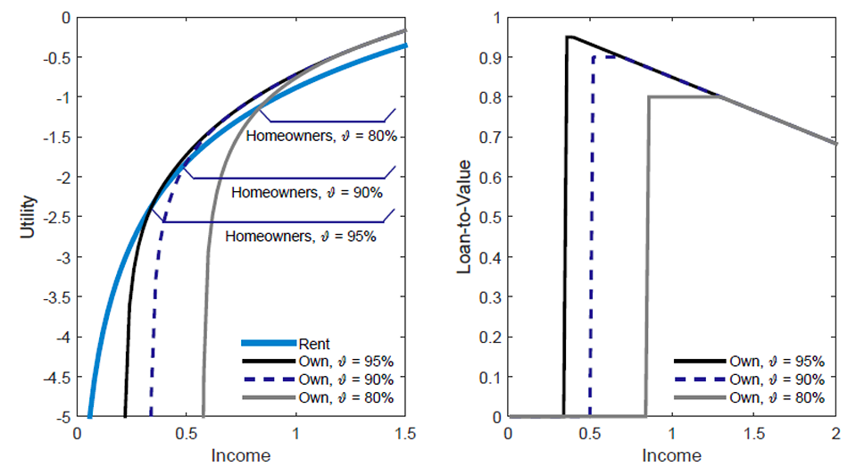
Note: The parameters are $\overline{a} = 1, h = 2.5, p = 1, r = 0.04, r_a = 0.05, \omega = 0.75, and \phi = 0.5$ .

The Quantitative Framework

The benchmark model is an infinite horizon, open endowment economy populated by a continuum of exante identical households and a competitive financial sector.

Households

Household preferences over numeraire consumption $c$ and shelter $s$ are given by

(6) $\begin{equation*} \begin{gathered} U(\{(c_t, s_t)\}\infty\limits_{t=0}) = \displaystyle\sum_{t=0}^{\infty} \beta^t^{\frac{([\omega c_t^{\frac{\epsilon - 1}{\epsilon}} + (1- \omega)s_{t}^{\frac{\epsilon - 1}{\epsilon}}]^{\frac{\epsilon}{\epsilon - 1}})^{1-\sigma}}{1 - \sigma}, \end{gathered} \end{equation*}$

where shelter can either be obtained period-by-period from apartment space or acquired by purchasing durable owner-occupied housing. Households are ex-ante identical but receive uninsurable, idiosyncratic shocks $e \cdot z$ to their endowment of the numeraire good. The persistent component $z \in Z$ follows Markov transitions $\pi_z (z^{\prime}|z)$ with stationary distribution $\Pi_z (z)$ , and the transitory component $e \in E$ is drawn from the cumulative distribution function $F(e)$ . To self-insure, households can save using risk-free bonds, and owners can borrow using mortgages.

The Markets for Shelter

Consistent with empirical evidence, the owner and rental markets are segmented by quality, with apartments $a \in [0, \overline{a}]$ inferior to houses $h \in H$ , i.e., $\overline{a} /leq minH \equiv h$ . ⁴ Apartment space provides shelter $s= a$ , is produced from the numeraire good using a linear technology at the rate $A$ , and is traded competitively at unit price $r_a = 1/A$ . ⁵

Houses require proportional holding costs $\delta$ each period (e.g., maintenance, property taxes, etc.), provide shelter $s = h$ , and are produced at marginal cost $p$ using a linear, reversible construction technology.⁶ Different from the Walrasian paradigm, housing trades are subject to endogenous delays and transaction costs that arise from search frictions. Hedlund (2016) goes into depth developing the microfoundations, but the essential overview is as follows. Aspiring sellers choose a list price $x_s$ and successfully trade with probability $\eta_s (x_s; p)$ . The larger discount sellers accept, $p - x_s)$ , the quicker they expect to sell. Buyers make a bid $x_b$ for house $h$ and buy with probability $\eta_b (x_b; p)$ , which increases in $x_b$ .

Financial Market Arrangements

Households save using one-period risk-free bonds and borrow using long-term defaultable mortgage contracts. Competitive banks intermediate all financial market trades with households and have access to external financing at exogenous interest rate $r$ . Thus, bonds are traded at price $q = \frac{1}{1+r}$ , while the more complicated mortgage pricing equation is given by equation (6) below.

The ability of borrowers to default is sometimes exercised in equilibrium. As a result, banks price this risk into new mortgages at origination, and borrowers face individually tailored prices $q_m(X)$ that reflect the default risk associated with their state vector $X=(m^{\prime}, b^{\prime},h, z)$ . Mathematically, when borrowers choose mortgage $m^{\prime}$ , they are taking on debt with face value $m^{\prime}$ that they gradually repay over the duration of the loan. In exchange for this “promised” repayment, the bank delivers $q_m(X)m^{\prime}$ in up-front resources. In subsequent periods, homeowners can choose from three options: default, refinance (i.e., pay off the existing loan and take out a new loan after paying a proportional origination cost $\zeta$ ), or make a regular payment $l \geq \underline{l}$ , where $\underline{l}$ is the minimum payment amount. Borrowers can then roll over unpaid balances at the rate $r_m = (1+r)(1+\phi)$ , where $\phi$ represents a loan servicing cost. Thus, for borrowers making regular payments, debt follows $m^{\prime} = (m-l)(1+r_m)$ .

Some clarifying remarks are in order. First, mortgages do not have fixed durations or face rigid amortization schedules in this setup. Besides facilitating computational tractability by shrinking the state space, this assumption implicitly stands in for the availability of additional mortgage instruments—second mortgages, home equity lines of credit, etc.—that allow borrowers to adjust the path of their cumulative debt.

Second, the long-term duration of mortgages ensures that down payment requirements only apply at origination. Importantly, existing borrowers are not expected to inject equity in the event that requirements tighten for any reason. In other words, there is no forced deleveraging. Similarly, if a borrower who initially appears safe at the time of mortgage origination subsequently experiences a negative shock that increases the difficulty of repayment, banks do not have the ability to adjust mortgage terms to reflect higher default risk. Lastly, again for reasons of tractability, all default risk is priced into $q_m(X)$ rather than in the rollover rate $r_m$ .

Consequences of Foreclosure

Defaulting borrowers lose their house and have a credit flag $f = 1$ placed on their record that excludes them from future borrowing until the flag disappears with probability $1 - \lambda_f$ . Banks manage the selling of their foreclosure (REO) properties subject to the same market frictions faced by other sellers. Banks also lose a fraction $\chi$ in foreclosure costs upon selling. The value of repossessing house $h$ is

(7) $\begin{equation*} J_{R E O}(h)=\max _{x_s \in\{\infty\} \cup \mathbb{R}^{+}} \underbrace{\eta_s\left(x_s, h\right)}_{\text {prob of selling }} \underbrace{(1-\chi) x_s}_{\text {revenue }}+\left[1-\eta_s\left(x_s, h\right)\right][\underbrace{-\delta p h}_{\text {maintenance }}+\frac{1}{1+r} J_{R E O}(h)] \text {, } \end{equation*}$

where $x_s = \inft$ indicates the choice to not list the house for sale at all. When housing market conditions are stable, banks always prefer to attempt a sale rather than continually pay maintenance and time costs on their inventories. However, banks may time the market strategically when housing conditions are in flux.

Mortgage Pricing

At the time of origination, mortgage prices reflect the external cost of financing to the bank, servicing costs, and borrower-specific default risk. Because mortgages are long-term contracts, competitive pricing is determined by the recursive equation

(8) $\begin{equation*} \begin{aligned} & (1+\zeta) q_m(X)=\frac{1}{1+r_m} \mathbb{E}\{\overbrace{\eta_s\left(x_s^{\prime}, h\right)}^{\text {sell + repay }}+\overbrace{\left[1-\eta_s\left(x_s^{\prime}, h\right)\right]}^{\text {no sale (fail/do not try) }}[\overbrace{d^{\prime} \min \left\{\frac{J_{R E O}(h)}{m^{\prime}}, 1\right\}}^{\text {default }}\} \\ & \left.\left.+\left(1-d^{\prime}\right)\{\underbrace{\mathbf{1}_{[\text {Refi }]}}_{\text {repay in full }}+\mathbf{1}_{\text {[No Refi] }}(\underbrace{l^{\prime}}_{\text {payment }}+\underbrace{(1+\zeta) q_m\left(X^{\prime}\right) \frac{m^{\prime \prime}}{m^{\prime}}}_{\text {continuation for } m^{\prime \prime}=\left(m^{\prime}-l^{\prime}\right)\left(1+r_m\right)})\}\right]\right\}, \\ & \end{aligned} \end{equation*}$

where $x^{\prime}_s$ is the household’s list price choice (which includes not listing at all), and $d^{\prime} \in \{0,1\}$ is the decision whether to default. The left side of (6) reflects expenditures per unit of $m^{\prime}$ by the bank at origination, and the right side equals expected discounted revenues. The law of large numbers ensures that banks earn zero profits loan-by-loan

Household Choices

At the beginning of each period, all households learn their endowment shocks $(e,z)$ and their credit status $f \in \{0,1\}$ . Homeowners then decide whether to list their house for sale and, if so, which list price $x_s$ to select. After selling outcomes are realized, remaining homeowners with mortgage debt choose whether to default, refinance, or make a regular payment. Afterwards, renters looking to buy enter the market and choose their desired house $h$ and bid price $x_b$ . Consumption and portfolio decisions are then made at the end of the period. In addition to $f \in \{0,1\}$ , the state vectors for homeowners and renters are $X_{own} = (y,m,h,z)$ and $X_{rent} = (y,z)$ , respectively, where cash at hand � represents the sum of the endowment $e \cdot z$ and bonds $b$ .

House Trading and Default Choices

The value function of owners at the beginning of the period with $f = 0$ is

(9) $\begin{equation*} \begin{aligned} W_{\text {own }}^0\left(X_{\text {own }}\right)= & \max _{x_s \in\{\infty\} \cup\left\{x_s+y \geq m\right\}} \eta_s\left(x_s, h\right) W_{\text {rent }}^0\left(y+x_s-m, z\right)+\left[1-\eta_s\left(x_s, h\right)\right] \\ & \times \max \left\{V_{\text {debt }}\left(X_{\text {own }}\right), V_{\text {own }}^0(y-m, h, z), W_{\text {rent }}^1(y, z)\right\} . \end{aligned} \end{equation*}$

Conditional on actively listing on the market, the constraint $x_s + y \geq m$ states that borrowers must pay off all outstanding mortgage debt at the time of sale. In the event that a homeowner does not sell (either by choice or bad luck), they choose between making a regular payment, paying off their entire debt $m$ with the option of subsequently originating a new loan, or defaulting and immediately becoming a renter with credit flag $f = 1$ . Implicitly, equation (7) restricts homeowners to choices that yield non-empty budget sets in the portfolio choice phase of the period.⁷

Owners with bad credit (and therefore no mortgage), $f = 1$ , have value function

(10) $\begin{equation*} W_{\text {own }}^1\left(X_{\text {own }}\right)=\max _{x_s \in\{\infty\} \cup \mathbb{R}^{+}} \eta_s\left(x_s, h\right) W_{\text {rent }}^1\left(y+x_s, z\right)+\left[1-\eta_s\left(x_s, h\right)\right] V_{\text {own }}^1(y, h, z) . \end{equation*}$

When facing the choice of whether or not to buy, renters solve

(11) $\begin{equation*} W_{\text {rent }}^f\left(X_{\text {rent }}\right)=\max _{\substack{h \in \emptyset \mathrm{U}, x_b \in \mathcal{B}^f(h, z)}} \eta_b\left(x_b, h\right) V_{\text {own }}^f\left(y-x_b, h, z\right)+\left[1-\eta_b\left(x_b, h\right)\right] V_{\text {rent }}^f\left(X_{\text {rent }}\right) . \end{equation*}$

For buyers with access to credit, the set $B^0 (h,z) = \{x_b \in R^+:y-x_b \geq y(h,z)\}$ , where $y(h,z) < 0$

captures the ability to borrow using mortgages. Buyers with no credit access can only buy using cash at hand, i.e., $B^1 (h,z) = \{x_b \in R^+:y-x_b \geq 0\}$ .

Consumption and Portfolio Allocation Choices

Renters choose bonds $b^{\prime}$ , consumption $c$ , and apartment space $a$

(12) $\begin{equation*} \begin{gathered} V_{\text {rent }}^f\left(X_{\text {rent }}\right)=\max _{\substack{b^{\prime} \geq 0, c \geq 0, a \in[0, \bar{a}]}} u(c, a)+\beta \mathbb{E} W_{\text {rent }}^{f^{\prime}}\left(X_{\text {rent }}^{\prime}\right) \text { subject to } \\ c+r_a a+q b^{\prime} \leq y \\ X_{\text {rent }}^{\prime}=\left(e^{\prime} z^{\prime}+b^{\prime}, z^{\prime}\right) . \end{gathered} \end{equation*}$

Owners with debt choose payment $l \geq \underline{l}, \text{ bonds } b^{\prime}, \text{ and consumption} c,$

(13) $\begin{equation*} \begin{gathered} V_{\text {debt }}\left(X_{\text {own }}\right)=\max _{\substack{l \geq l, b^{\prime} \geq 0, c \geq 0}} u(c, h)+\beta \mathbb{E} W_{o w n}^0\left(X_{o w n}^{\prime}\right) \text { subject to } \\ c+\delta p h+q b^{\prime}+l \leq y \\ X_{\text {own }}^{\prime}=\left(e^{\prime} z^{\prime}+b^{\prime},(m-l)\left(1+r_m\right), h, z^{\prime}\right), \end{gathered} \end{equation*}$

where $l \equiv \frac{r_m}{1+r_m}m$ is the interest-only minimum down payment. Owners with access to credit but no current mortgage choose loan $m^{\prime}$ , bonds $b^{\prime}$ , and consumption $c$ ,

(14) $\begin{equation*} \begin{gathered} V_{o w n}^0(y, h, z)=\max _{\substack{m^{\prime} \geq 0, b^{\prime} \geq 0 \\ c \geq 0}} u(c, h)+\beta \mathbb{E} W_{o w n}^0\left(X_{o w n}^{\prime}\right) \text { subject to } \\ c+\delta p h+q b^{\prime} \leq y+q_m\left(m^{\prime}, b^{\prime}, h, z\right) m^{\prime} \\ q_m\left(m^{\prime}, b^{\prime}, h, z\right) m^{\prime} \leq \vartheta p h \\ X_{o w n}^{\prime}=\left(e^{\prime} z^{\prime}+b^{\prime}, m^{\prime}, h, z^{\prime}\right), \end{gathered} \end{equation*}$

where \upsilon is the maximum loan-to-value ratio. For owners without credit access,

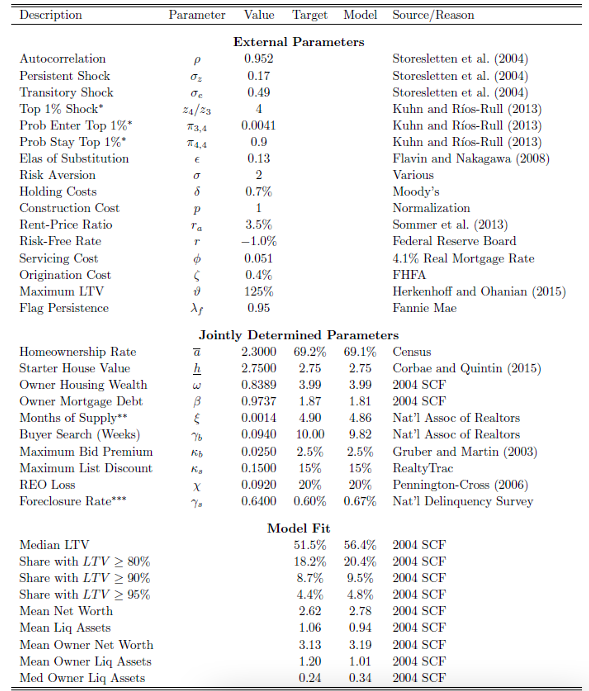
(15) $\begin{equation*} \begin{gathered} V_{o w n}^1(y, h, z)=\max _{b^{\prime} \geq 0, c \geq 0} u(c, h)+\beta \mathbb{E} W_{o w n}^{f^{\prime}}\left(X_{o w n}^{\prime}\right) \text { subject to } \\ c+\delta p h+q b^{\prime} \leq y \\ X_{o w n}^{\prime}=\left(e^{\prime} z^{\prime}+b^{\prime}, m^{\prime}=0, h, z^{\prime}\right) . \end{gathered} \end{equation*}$

Disciplining the Model

This section follows in setting the model parameters to match features of the US economy prior to the 2007–2011 housing crash. Some parameters are taken directly from the data or relevant literature, while the remaining parameters are determined jointly within the model. Table 1 provides a summary.

External Parameters

The parameters for the stochastic endowment $e \cdot z$ come from adapting Storesletten, Telmer, and Yaron (2004) to a quarterly setting and normalizing annual income to 1 using the procedure of Hedlund (2018). Following Castañeda, Díaz-Giménez, and Ríos-Rull (2003), a fourth persistent income state is introduced for the top 1 percent to better match wealth inequality from the data. Risk aversion is set to $\sigma = 2$ , and the elasticity of substitution between consumption and shelter is $\epsilon$ = 0.13, following Flavin and Nakagawa (2008) and Kahn (2009). However, the results also analyze an alternative Cobb-Douglas calibration. The discount factor $\beta$ is determined jointly.

Construction costs are normalized to $p = 1$ , and the annual price of apartment space is $r_a = 0.035$ to yield a 3.5 percent rent-price ratio. The mapping from $p$ to $eta_s(\cdot;p)$ and $\eta_b(\cdot;p)$ emerges from directed search and free-entry of market makers who facilitate trades between sellers and buyers. Hedlund (2016) gives more details of the search environment, but here, it suffices to present the reduced-form expressions

$\begin{gathered} \eta_s\left(x_s ; p\right)=\min \left\{1, \max \left\{0,\left(\frac{p-x_s}{\kappa_s h}\right)^{\frac{\gamma_s}{1-\gamma_s}}\right\}\right\} \\ \eta_b\left(x_b ; p\right)=\min \left\{1, \max \left\{0,\left(\frac{x_b-p}{\kappa_b h}\right)^{\frac{\gamma_b}{1-\gamma_b}}\right\}\right\}, \end{gathered}$

where the parameters $\gamma_s, \gamma_b, k_s, \text{ and } k_b$ are determined jointly. In addition, a small utility cost $\zeta$ of failing to sell is introduced; this is to prevent homeowners (especially those on the fence about selling) from setting a list price that leads to a house staying on the market for an extremely long time.

Consistent with the low interest rate environment of the mid-2000s, the annual real risk-free rate is −1 percent, the annual servicing cost is $\phi$ = 0.051 to generate a 4.1 percent real mortgage rate, and the origination cost is $\zeta$ = 0.4 percent. The maximum loan-to-value is set at a non-binding 125 percent to reflect the popularity of high leverage loans prior to the housing bust documented by Herkenhoff and Ohanian (2015). Lastly, the credit flag persistence $\gamma_f$ = 0.95 corresponds to an expected five-year wait before foreclosed borrowers regain access to credit, and the REO discount $x$ is determined jointly.

Jointly Determined Parameters

The joint calibration sets out to match moments of the data circa mid-2000s related to the housing market and portfolio holdings reported by the 2004 Survey of Consumer Finances. Regarding the housing market, particular attention is paid to matching foreclosure activity along with price spreads and trading delays from search frictions. As shown in table 1, the model replicates debt and asset holdings remarkably well.

Table 1. Model Calibration

Results

To determine the sensitivity of homeownership to credit constraints, the quantitative experiments analyze the dynamic response of the model economy to an unexpected, permanent tightening of down payment requirements. The benchmark results assume constant marginal cost reversible construction, which fixes $p$ and gives an upper bound for the homeownership response. Later, the opposite case of a fixed total housing stock is briefly considered where price changes blunt the adjustment in quantities.

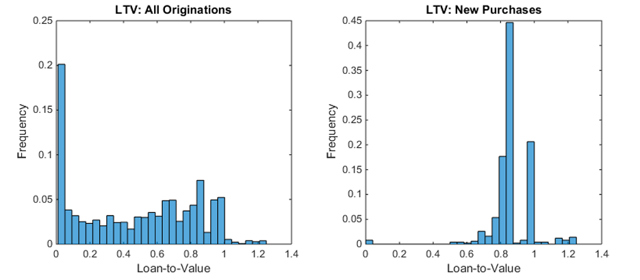
Recall that, in the benchmark calibration, mortgages are limited to 125 percent loan-to-value at origination. However, figure 3 demonstrates that this constraint is essentially non-binding. The left panel, which lumps together refinance and purchase loans, shows a sharp drop off above 100 percent LTV. Even without a constraint, most borrowers avoid these negative equity loans because banks embed a steep default premium into the mortgage price $q_m(\cdot)$ . The right panel shows a similar drop-off for purchase loans, with significant bunching just to the right of 80 percent LTV and to the left of 100 percent LTV.

Figure 3. (Left) Loan-to-Value Distribution for All New Mortgage Originations; (Right) Loan-to-Value Distribution for New Purchase-only Loans

Given this bunching and the historical popularity of 20 percent down payment loans, the first experiment analyzes the dynamic effects of reducing the maximum leverage at origination to 80 percent. The experiment is then repeated with a more severe 50 percent minimum down payment requirement to investigate potential nonlinearities in the homeownership response. To assess the importance of substitutability between housing and consumption, a re-calibrated Cobb-Douglas specification is subjected to the same experiments. Lastly, all of the above is run again using an analogous pair of stylized life-cycle economies to test robustness and to provide insight about the impact of credit constraints on households at different stages of their lives.

Down Payments and the Importance of Time Horizon

After the imposition of a 20 percent minimum down payment, the homeownership rate declines gradually by 2.4 percentage points over the next three years. In the cross section, the largest drop occurs among middle-income households occupying small houses, whereas low income renters and upper income homeowners barely change tenure status. Although these results align well with the static model intuition, focusing only on the trough gives an incomplete and misleading picture about the relationship between minimum down payments and homeownership.

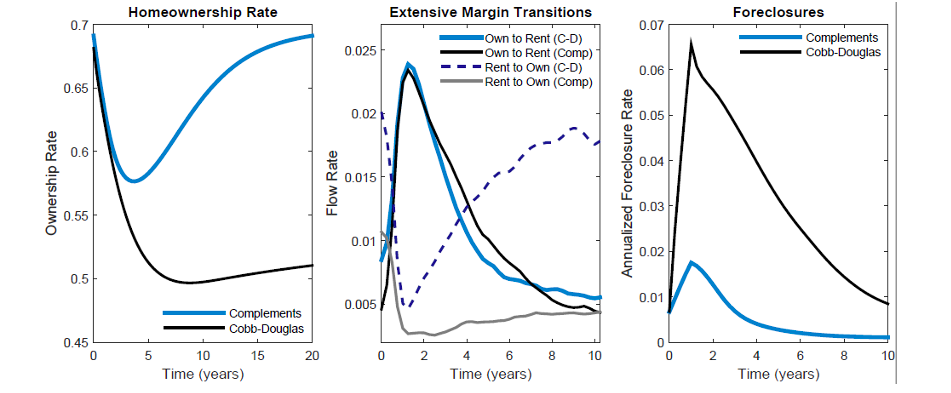
Figure 4. (Left) Total Homeownership Rate; (Middle) Transitions between Owning and Renting; (Right) Upsizers and Downsizers

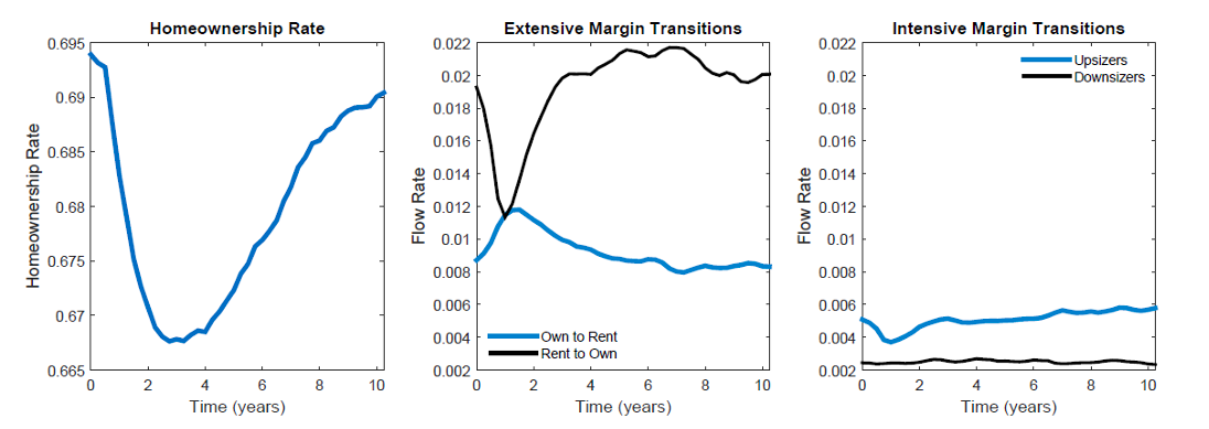
Figure 4 shows that the homeownership rate almost completely recovers after 10 years. Furthermore, the temporary decline comes more from a depressed flow of renters into homeownership than from an exodus of homeowners into renting. In fact, the entire increase in the own-to-rent rate occurs among borrowers with leverage above 75 percent, but they account for a smaller fraction of homeowners over time. The long-term nature of mortgage contracts is key to this result, with collateral requirements applied only upon origination of new loans and not to existing borrowers. For the same reason, panel 3 reveals that higher down payment requirements slow movement up the property ladder without increasing the fraction of homeowners who downsize.

Transitioning from the Short Run to the Long Run

Multiple factors account for the long-run resilience of the homeownership rate to tighter credit. First, the non-degenerate portfolio choice problem implies that borrowing-constrained households are not necessarily the same as those on the margin between buying and renting. Recall that, in the initial equilibrium, the overwhelming majority (86 percent) of new purchases are made with less than a 20 percent down payment. Yet when the 20 percent minimum is imposed, rent-to-own transitions fall by less than half, and fewer than 5.4 percent of buyers are completely shut out by an empty budget set.

Instead, most buyers prefer to have resources left over for saving, which creates another margin for adjustment other than forgoing the decision to buy.

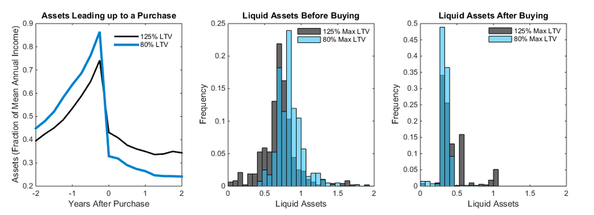
Figure 5. (Left) Liquid Assets of New Buyers Leading up to the Date of Purchase; (Middle and Right) Distribution of Assets before and after Purchase, Respectively

Furthermore, because they face the lowest default premia, upper-income buyers actually take out the most leverage at the time of purchase. The average loan-to-value for lower-income, middle-income, and upperincome buyers is initially 77 percent, 84 percent, and 97 percent, respectively. Yet even while upperincome buyers are the most borrowing constrained after down payments increase, their homeownership rate remains stable.⁸

The ability to gradually save for a down payment is also a long-run stabilizing force for homeownership. Panel 1 of figure 5 shows asset dynamics leading up to a new home purchase. More stringent down payment requirements create a longer build-up period followed by a steeper decline after buying. The middle panel illustrates the cross-sectional increase in asset accumulation before buying, and the right panel exhibits the post-purchase decline. Thus, just as in prototypical one-asset incomplete markets models, agents build savings to buffer themselves against the constraint.

Homeownership with Very Large Down Payment Requirements

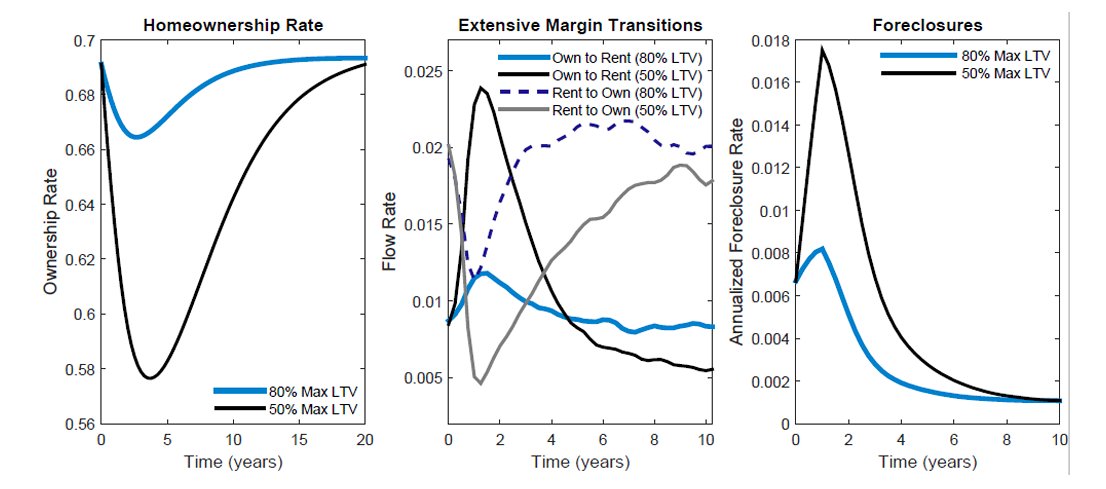
The same dichotomy between short-run and long-run dynamics occurs after raising the down payment requirement to a more severe 50 percent. Moreover, the magnitude of the short-run homeownership response is highly nonlinear with respect to the stringency of borrowing constraints. Upon imposition of the tighter limits for new loans, the share of existing borrowers with leverage above the threshold is three times larger in the 50 percent case compared to the 20 percent case, but the short-run decline in homeownership is nearly five times as large and much more protracted, as shown by the left panel of figure 6. Also, recall that implementing a 20 percent minimum down payment prompted a fall in the rate of rent-to-own transitions with only a modest rise in own-to-rent flows. However, the middle panel demonstrates that a more severe tightening of credit causes a temporary surge in the flow of homeowners switching to renting. A portion of this exodus comes from foreclosures, as indicated by the right panel, although these “involuntary” flows are stable between 15 percent and 20 percent of all own-to-rent transitions.

Figure 6. Comparison of the Response to a 20% vs. 50% Minimum Down Payment

What accounts for the nonlinear homeownership response? First, the decision to default is a nonlinear function of home equity that depends on credit access. When borrowing limits tighten, homeowners with leverage above the new threshold can no longer respond to negative shocks by extracting equity through refinancing. The only remaining consumption-smoothing avenues are to sell or default. Homeowners prefer to sell, but debt overhang from the list price constraint $x_s + y \geq m$ exacerbates illiquidity-induced trading delays and pushes some unsuccessful sellers into default.

Long-term debt represents a second source of nonlinearities. Figure 11 in the appendix shows that homeowners who become constrained by tighter credit do not simply bunch at the borrowing constraint. Instead, mass accrues throughout the entire left tail of the leverage distribution, which pushes down the average loan-to-value to 25 percent—far below the constraint. Even though most buyers make close to the minimum down payment, they gradually build equity over time, which is costly for them to extract through repeated refinancing. This prolonged period of asset accumulation prior to purchasing also explains the slow recovery in homeownership.

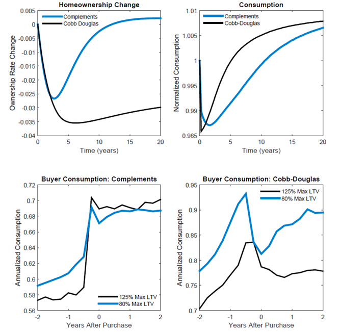
Figure 7. Comparison between the Benchmark and Cobb-Douglas Calibrations of the Response to a 20% Down Payment Requirement

Housing and Consumption: The Role of Substitution

The benchmark results—which feature housing and consumption as complements in the utility function—reveal a strong interplay between the homeownership rate and down payment requirements in the short run but no relationship in the long run. Figure 7 shows how these results hold up in the case of a 20 percent minimum down payment when the model is re-calibrated using a Cobb-Douglas specification. Qualitatively, the top left panel reveals that a higher degree of substitutability causes homeownership to remain permanently lower after a tightening of credit, though the pattern of overshooting and partial recovery still exists. Quantitatively, however, the impact of reducing the maximum leverage from 125 percent to 80 percent only reduces the homeownership rate by 2.6 percentage points in the long run.

The remaining panels in figure 7 provide insight into how the dynamics of consumption under the two specifications differ and shape the resulting homeownership response. After an initial decline, consumption recovers much more rapidly with greater substitutability in preferences. With strong complementarity, households tolerate lower consumption while they build up assets for a larger down payment, whereas households in the Cobb-Douglas specification are more willing to shift from housing toward consumption.

Figure 8. Comparison between the Benchmark and Cobb-Douglas Calibrations of the Response to a 50% Down Payment Requirement

The dynamics of consumption also exhibit significant differences between the two specifications surrounding the date of a house purchase. With complementary preferences and loose credit, consumption is flat leading up to the point of purchase and then jumps in tandem with the increase in shelter from houses being larger than apartments, $h > \overline{a}$ . Tightening down payments in this environment attenuates the jump in consumption upon purchase. By contrast, with greater substitutability in preferences, consumption grows more steeply during the asset build-up phase before falling at the time of purchase. When down payments are tightened in this case, the path of consumption before and after purchase shifts upward, caused mostly by a composition effect from a shift in the pool of buyers towards higher income.

Substitutability in the Midst of a Severe Credit Tightening

Nevertheless, for the central question at hand about the relationship between homeownership and down payments, neither specification predicts a strong long-run response to the introduction of a 20 percent minimum down payment. This parity quickly breaks down, however, if a severe 50 percent down payment requirement is introduced, as shown by figure 8. The left panel shows that homeownership drops to 50 percent with Cobb-Douglas preferences and remains permanently depressed. The middle panel gives some clues into the anatomy of this decline. Under both specifications, the rate of own-to-rent transitions temporarily increases before eventually reverting to its original level. However, in the Cobb-Douglas environment, approximately 60 percent of the homeownership exodus is attributable to foreclosures, which spike to a level three times higher than in the benchmark calibration. More importantly, the flow of renters into homeownership collapses in the Cobb-Douglas economy and never recovers, which is the crux of why homeownership stays low.

Long-Run Ownership: Credit Limits vs. Interest Rates

Barring a return to the pre-Great Depression mortgage environment, 50 percent minimum down payments are unlikely to ever again become a reality.⁹ Otherwise, sections 5.1 and 5.2 show that the longterm impact of implementing a 20 percent minimum down payment—still a significant departure from current credit limits—would be modest or nil, depending on the preference specification. However, these findings do not imply that the homeownership rate is independent of credit entirely. To the contrary, changes in interest rates have long-run effects on homeownership. In the benchmark calibration, increasing interest rates by 2 percent causes homeownership to fall by 5.6 percent in the short run and 3 percent in the long run.¹⁰ Likewise, reducing rates from an initially higher level produces the mirror image result. Thus, the rise in the US homeownership rate between 1998 and 2006 can be viewed through the lens of the model as some combination of a temporary response to looser down payment requirements and a permanent response to lower interest rates. Since then, numerous changes in the housing and mortgage environment have likely conspired to suppress homeownership, despite the continuation of low borrowing costs.

House Prices and Inelastic Supply

To maximize the response of quantities rather than prices to changes in down payment requirements, the analysis to this point has featured a constant marginal cost $p$ for the reversible construction technology. However, even with the deck stacked in this manner, introducing a 20 percent down payment requirement has had little long-run impact on the homeownership rate. This section briefly considers the opposite case of a fixed total housing stock. The appendix provides the housing market clearing condition.¹¹

Figure 9. Comparison between the Benchmark and Cobb-Douglas Calibrations of the Response to a 50% Down Payment Requirement with Inelastic Supply

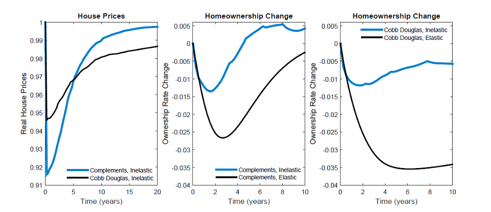
As one might expect, figure 9 confirms that house prices decline after the imposition of a 20 percent down payment requirement, and the reduction in prices attenuates the fall in homeownership. Regardless of the specification for preferences, homeownership only falls by 1 percent in the short run and returns approximately to its initial level in the long run. For the benchmark calibration, house prices also return to their initial level in the long run after falling by 8 percent upon initiation of the tighter down payments. The Cobb-Douglas specification yields a smaller price decline on impact but a slower and incomplete recovery, ending 1 percent below the starting point.

Homeownership, Asset Accumulation, and the Life Cycle

The decision of households to gradually build savings in the face of higher down payment requirements explains the resilience of homeownership to tighter credit. However, what if, unlike in an infinite horizon environment, households “run out of time” to accumulate assets for a home purchase? To answer this question, a stylized life cycle dimension is added to the model. Specifically, agents now face stochastic death each period with an annualized probability of $p$ = 0.975, which corresponds to an expected life span of 40 years. Upon death, all home equity and liquid assets are expunged, and homeowners’ houses are auctioned off to cover any outstanding debt. All dead households are replaced by newborn renters with zero savings starting at the lowest persistent income state. Thus, even without an age-specific deterministic wage profile, newborn households anticipate a rising income profile and greater future saving. To maximize the impact of credit constraints, households are not permitted to make bequests or inter vivos transfers.¹²

Table 2. Homeownership Response to a 20% Minimum Down Payment

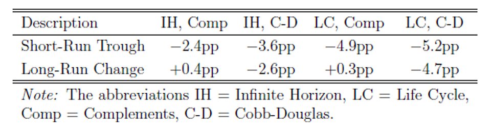
Table 3 in the appendix gives the calibration parameter values, and table 2 summarizes the behavior of homeownership for each case. With a 20 percent down payment requirement, life cycle behavior magnifies the short-run homeownership decline but does nothing to alter its long-run stability when housing and consumption are complements. With Cobb-Douglas utility, the life cycle—even with its exaggerated assumption of no bequests or inter vivos transfers—only reduces long-term homeownership by 2.1 percent.

Figure 10. (Left) Housing Transitions after Imposing a 50% Minimum Down Payment with Complements; (Middle) Homeownership by Age; (Right) Liquid Assets by Age

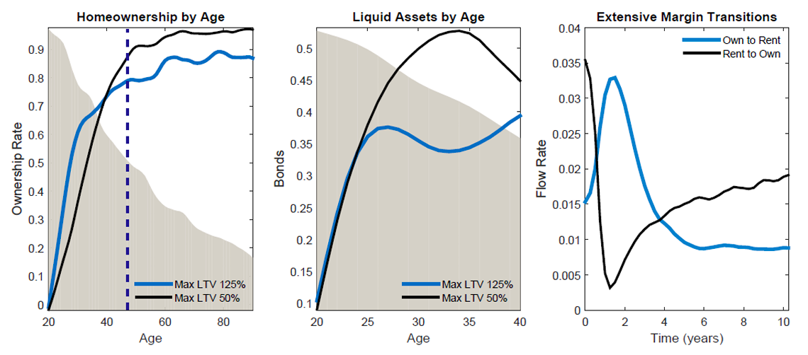
Note: The shaded area is the age distribution. The dashed line is the median age.

Even with a 50 percent down payment requirement, the life cycle model with complementarity between housing and consumption still only experiences a long-run homeownership decline of 2 percent. However, the left panel of figure 10 shows that this aggregate stability conceals significant heterogeneity by age. Homeownership among the young declines precipitously because of the added time required to accumulate assets for a larger down payment. The middle panel confirms this increased savings behavior among households at the age where they are preparing to buy. However, by around age 40, the homeownership rate in the economy with tighter down payments starts to exceed that of the low down payment economy. The right panel gives some clues as to the reason. Consistent with earlier intuition, higher down payments reduce rent-to-own flows by complicating the path for aspiring buyers into homeownership. However, precisely because higher down payments make transitioning from renting to owning more difficult, homeowners are more reluctant to ever transition into renting. In other words, own-to-rent flows fall as well. The result is a significant dampening of gross flows in both directions that produces little change in net flows or homeownership. Notably, Boehm and Schlottman (2014) find cross-country empirical evidence in support of this negative relationship between down payment requirements and gross housing tenure flows.

Conclusions

The bottom line that emerges from this analysis is one of a highly time-dependent relationship between credit constraints and homeownership. In the short run, tighter down payments depress homeownership as in the static model of section 2. However, with moderate down payment requirements on the order of 20 percent, the relationship largely disappears in the long run. A significant long-run link between down payments and homeownership only emerges after an implausibly severe contraction in borrowing limits, and even then, only if preferences feature a substantial degree of substitutability between housing and consumption. Explicitly modeling the life cycle, even with exaggerated assumptions limiting bequests and inter vivos transfers, mostly just alters short-run dynamics. Overall, the main results and the robustness checks backing them up signal that fears about the threat of down payments to long-run homeownership may be exaggerated, though policymakers and researchers interested in debt-reducing macroprudential policies should be mindful of the transitional dynamics associated with such interventions.

References

Acolin, Arthur, Jesse Bricker, Paul Calem, and Susan Wachter. 2017. “Borrowing Constraints and Homeownership Over the Recent Cycle.” Working Paper.

Anenberg, Elliott, Aurel Hizmo, Edward Kung, and Raven Molloy. 2017. “Measuring Mortgage Credit Availability: A Frontier Estimation Approach.” Working Paper.

Bachmann, Rudiger, and Daniel Cooper. 2014. “The Ins and Arounds in the US Housing Market.” Working Paper.

Boehm, Thomas P., and Alan M. Schlottmann. 2014. “The Dynamics of Housing Tenure Choice: Lessons from Germany and the United States.” Journal of Housing Economics 25:1–19.

Castañeda, Ana, Javier Díaz-Giménez, and José-Víctor Ríos-Rull. 2003. “Accounting for the US Earnings and Wealth Inequality.” Journal of Political Economy 111 (4): 818–57.

Chambers, Matthew, Carlos Garriga, and Don E.Schlagenhauf. 2009. “Accounting for Changes in the Homeownership Rate.” International Economic Review 50 (3): 677–726.

Chiuri, Maria Concetta, and Tullio Jappelli. 2003. “Financial Market Imperfections and Home Ownership: A Comparative Study.” European Economic Review 47:857–75.

Corbae, Dean, and Erwan Quintin. 2015. “Leverage and the Foreclosure Crisis.” Journal of Political Economy 123:1–65.

Davis, Morris A., Andreas Lehnert, and Robert F. Martin. 2008. “The Rent-Price Ratio for the Aggregate Stock of Owner-Occupied Housing.” Review of Income and Wealth 54 (2): 279–84.

Engelhardt, Gary V. 1996. “Consumption, Down Payments, and Liquidity Constraints.” Journal of Money, Credit, and Banking 28 (2): 255–71.

Flavin, Marjorie, and Shinobu Nakagawa. 2008. “A Model of Housing in the Presence of Adjustment Costs: A Structural Interpretation of Habit Persistence.” American Economic Review 98, no. 1 (March): 474–95.

Gete, Pedro, and Franco Zecchetto. 2018. “Distributional Implications of Government Guarantees in Mortgage Markets.” Review of Financial Studies 31 (3): 1064–97.

Gete, Pedro, and Michael Reher. 2016. “Two Extensive Margins of Credit and Loan-to-Value Policies.”

Journal of Money, Credit, and Banking 48 (7): 1397–1438.

———. 2018. “Mortgage Supply and Housing Rents.” Review of Financial Studies 31 (12): 4884–911.

Glaesar, Edward L., and Joseph Gyourko. 2007. “Arbitrage in Housing Markets.” NBER Working Paper no. w13705, National Bureau of Economic Research, Cambridge, MA, January 2007.

Goodman, Laurie S., and Christopher Mayer. 2018. “Homeownership and the American Dream.”

Journal of Economic Perspectives 32, no. 1 (Winter): 31–58.

Gruber, Joseph, and Robert F. Martin. 2003. “The Role of Durable Goods in the Distribution of Wealth: Does Housing Make Us Less Equal?.” Working Paper.

Grundl, Serafin, and You Suk Kim. 2018. “The Effect of Government Mortgage Guarantees on Homeownership.” Working Paper.

Guiso, Luigi, and Tullio Jappelli. 2002. “Private Transfers, Borrowing Constraints, and Timing of Homeownership,” Journal of Money, Credit, and Banking 34 (2): 315–39.

Gyourko, Joseph, and Todd Sinai. 2004. “The (Un)Changing Geographical Distribution of Housing Tax Benefits: 1980 to 2000.” In vol. 18 of Tax Policy and the Economy, edited by James Poterba, 175–208. Cambridge, MA: MIT Press.

Halket, Jonathan, Lars Nesheim, and Florian Oswald. 2017. “The Housing Stock, Housing Prices, and User Costs: The Roles of Location, Structure, and Unobserved Quality.” Working Paper.

Haurin, Donald R., Patric H. Hendershott, and Susan M. Wachter. 1997. “Borrowing Constraints and the Tenure Choice of Young Households.” Journal of Housing Research 8 (2): 137–54.

Head, Allen, Huw Lloyd-Ellis, and Derek Stacey. 2018. “Inequality, Frictional Assignment, and Homeownership.” Working Paper.

Hedlund, Aaron. 2016. “Illiquidity and Its Discontents: Trading Delays and Foreclosures in the Housing Market.” Journal of Monetary Economics 83:1–13.

———. 2018. “Failure to Launch: Housing, Debt Overhang, and the Inflation Option.” ADEMU Working Paper 2018/098, January 2018.

Herkenhoff, Kyle, and Lee Ohanian. 2015. “The Impact of Foreclosure Delay on US Employment.” Working Paper.

Kahn, James A. 2009. “What Drives Housing Prices?.” Working Paper.

Kaplan, Greg, Kurt Mitman, and Giovanni L. Violante. 2017. “The Housing Boom and Bust: Model Meets Evidence.” Working Paper.

Kuhn, Moritz, and José-Víctor Ríos-Rull. 2013. “2013 Update on the US Earnings, Income, and Wealth Distributional Facts: A View from Macroeconomics.” Working Paper.

Li, Wenli, Haiyong Liu, Fang Yang, and Rui Yao. 2016. “Housing over Time and over the Life Cycle: A Structural Estimation.” International Economic Review 57 (4): 1237–60.

Mayer, Christopher J., and Gary V. Engelhardt. 1996. “Gifts, Down Payments, and Housing Affordability.” Journal of Housing Research 7 (1): 59–77.

Ortalo-Magné, François, and Sven Rady. 1999. “Boom In, Bust Out: Young Households and the Housing Price Cycle.” European Economic Review 43:755–66.

———. 2006. “Housing Market Dynamics: On the Contribution of Income Shocks and Credit Constraints.” The Review of Economic Studies 73, no. 2 (April): 459–85.

Pennington-Cross, Anthony. 2006. “The Value of Foreclosed Property.” JRER 28 (2): 193–214.

Sommer, Kamila, Paul Sullivan, and Randal Verbrugge. 2013. “The Equilibrium Effect of Fundamentals on House Prices and Rents,” Journal of Monetary Economics 60 (7): 854–70.

Storesletten, Kjetil, Chris I. Telmer, and Amir Yaron. 2004. “Cyclical Dynamics in Idiosyncratic Labor Market Risk,” Journal of Political Economy 112 June (3), 695–717.

Down Payments and the Homeownership Dream: Not Such a Barrier After All?

Executive Summary

Resources

Focuses

House/Senate Committees

Federal Agencies