Does Free Information Provision Crowd Out Costly Information Acquisition? It’s a Matter of Timing

Rentschler, Lucas; Aycinena Abascal, Diego; Elbittar, Alexander; Gomberg, Andrei

Introduction

Providing easily digestible information to “nudge” individual behavior has recently become a major theme in the literature on consumer choice.¹ It has also been demonstrated to play an important role in improving political choices.² An underexplored issue is the impact that such exogenous information provision may have on incentives for costly information acquisition that individuals could undertake on their own. At first glance, it may appear that the promise of free information would simply crowd out costly information acquisition. However, it turns out that for this to be true, the agent must be indifferent between actions so that an arbitrarily small amount of information would be decisive. Since this relies on initial exact indifference, it would not be something one could expect to observe often in real life.

In the absence of exact indifference, the promise of free information in the future can incentivize the agent to acquire more information than they would otherwise. The intuition for this result is grounded in the fact that information that does not affect one’s choice has no (instrumental) value. Unless one is ex ante indifferent, a small amount of information will do little to change posterior beliefs and will therefore not affect choices. That is, weak signals do not affect optimal behavior and are payoff irrelevant ex post, no matter their realization. This gives rise to the Radner and Stiglitz (1984) observation that the marginal value of small amounts of information is almost always zero. Thus, individual demand for information would normally exhibit discontinuities at zero since there is a minimum scale at which information should be acquired. This is the well-known Radner-Stiglitz nonconcavity in the value of information.³

A promise of delivering free additional information after an agent completes her costly acquisition can “smooth out” this nonconcavity. Indeed, if an agent knows that additional information will be provided, any information she acquires on her own will be valuable with positive probability so that the marginal value of a small amount of information is also positive. Hence, the promise of free information can stimulate acquiring small amounts of information, which otherwise should never be acquired.

In this paper, we provide a model of costly information acquisition in which agents are promised free information in the future, and test the predictions of this model in the lab. In our experimental design, subjects must choose between two options that are equally likely to be correct and can purchase information relevant to this decision. They also know that some relevant information will be provided for free. We vary the timing with which this free information is observed. In particular, the free information is provided before or after the information acquisition decision, or half is provided before and half after. Since free information that is observed before individual information acquisition can lead to updated priors, our design features both symmetric priors and asymmetric priors.

We conducted two waves of data collection. In the first, the timing of information acquisition was varied between subjects, while in the second, it was varied within subjects. Our experimental design across two waves allows us to explore the predictions of the model using both between- and within-subject variation. The results, both at the aggregate and the individual level, are qualitatively consistent with the predictions of the model: we find that when priors are asymmetric, subjects acquire more information when information is promised in the future. However, when priors are symmetric, the opposite is true.

The potential complementarity between free information and incentives for information acquisition has not, to the best of our knowledge, been clearly stated or tested. However, our work relates to the recent theoretical and experimental work on rational inattention (Caplin and Martin, 2015; Caplin and Dean, 2015; Caplin and Martin, 2018; Dean and Neligh, 2017). Similar to these studies, we explore the consequences of agents rationally deciding how much costly information to acquire. Promising additional information in the future allows us to directly vary the set of available informational strategies. The interaction between individual information acquisition and the timing of free information provision that we explore here may be seen as a novel implication of rational inattention.⁴ Our experimental test also relates to recent laboratory studies on costly information acquisition in collective decision-making (Bhattacharya et al., 2017; Elbittar et al., 2020; Grosser and Seebauer, 2016).⁵

Theory

We consider a simple model of information acquisition with two possible states of the world, $\Omega =\left\{ R,B\right\}$ , and two possible actions, $a\in \left\{ r,b\right\}$ .⁶ A risk-neutral agent, who assigns a prior probability $P\left( R\right) =\beta \in \left( 0,1\right)$ to $\omega =R$ , chooses action $a$ , and her utility, $U$ , depends only on $a$ and $w$ .⁷

We assume that decision-making is different between the two states as long as her decision is correct. Specifically, we assume that $U\left( R,r\right) =U\left( B,b\right) =0$ . Her attitude toward the two possible errors may differ so that $U\left(B,r\right) =-q$ and $U\left( R,b\right) =-\left( 1-q\right)$ . With these parameters, the agent would be willing to choose $a=r$ if and only if $P\left( R\right) \geq q$ . Thus $q\in \left( 0,1\right)$ may be interpreted as the degree of certainty necessary for the agent to choose $a=r$ .

Each signal $S_{i}\in \{\hat{r},\hat{b}\}$ is binary and correlated with the state of the world so that $P(S_{i}=% \hat{r}|\omega =R)=P(S_{i}=\hat{b}|\omega =B)=p\in \left( \frac{1}{2},1\right)$ . Conditional on the state, signals are independent and identically distributed (i.i.d). Before choosing $a$ , the agent decides how many signals she would like to produce, $v$ , at a constant per-signal cost $c>0$ . She also knows that a fixed number of free signals, $n$ , will be observed after she chooses how many signals to purchase but before she chooses $a$ . We concentrate on the interaction between the timing at which the free signals are observed by the agent and her decision to acquire additional signals.

The posterior belief of a Bayesian agent who observes $m$ signals $S_{i}=%\hat{r}$ and $k<m$ signals $S_{i}=\hat{b}$ is

$P\left( R|m\text{ signals }\hat{r}\text{ and }k<m\text{ signals }\hat{b}% \right) =\frac{\beta p^{m-k}}{\beta p^{m-k}+\left( 1-\beta \right) \left(1-p\right) ^{m-k}}.$

Since utility $U$ depends only on $a$ and $omega$ , information only has an instrumental value. It is only ex ante valuable if it has the potential to change an agents action, $a$ . The agent changes an action when $E[U(\omega,r)|$signals$]>E[U(\omega,b)|$signals$]$ .⁸ Thus, the smallest number of signals such that observing them has ex ante positive value is

$n^{\ast }=\min \left\{ k\in \mathbb{N}:\frac{\beta p^{n}}{\beta p^{n}+\left( 1-\beta \right) \left( 1-p\right) ^{k}}>q>\frac{\beta \left( 1-p\right) ^{n}% }{\beta \left( 1-p\right) ^{n}+\left( 1-\beta \right) p^{n}}\right\}\cdot$

As long as $\beta \neq q$ and $p$ is close enough to $\frac{1}{2}$ (i.e., information comes in small increments), $n^{\ast }>1$ : small amounts of information are useless. This is the manifestation of the Radner-Stiglitz nonconcavity in our setting. On the other hand, as long as the agent observes $N\geq n^{\ast }-1$ signals in addition to whatever information she acquires, even a single signal will always have a positive value. Thus, provided $c$ is sufficiently small, the promise of free signals will increase the level of costly information acquisition. Since acquiring a single signal is useless without the promise of free signals, the free signals cannot displace the agent’s own information acquisition effort; it can only be complementary to it.

There is, however, a special case in which any small amount of information is ex ante valuable. This happens if $\beta =q$ so that without observing any signals, the agent is indifferent between the two actions. In this case, standard Bayesian updating implies that she would choose $a=r$ whenever $m\equiv \#\{i:S_{i}=\hat{r}\}$ is bigger than $k\equiv \#\{i:S_{i}=\hat{b}\}$ and would choose $a=b$ whenever $k>m$ (the agent is indifferent whenever $k=m$ ). If $\beta =q$ , then standard Bayesian updating coincides with the simple “count-the-signals” rule of thumb, greatly simplifying the decision the agent faces. Notably, however, this is also the case in which observing even a single signal would break the indifference so that the marginal value of information at zero is, in fact, positive. This leads to a reversal of the expected impact of promising free signals: there is no nonconcavity in the value of purchased signals to smooth via the promise of free signals, and the agent is predicted to “free ride” on this promise.

Except in the knife-edge case outlined above, the promise of $n$ free signals can induce greater information acquisition. While we are primarily interested in testing this result, it is worth noting that the increased information acquisition will not improve the expected quality of the agent’s decisions. To see this, suppose the $n$ tree signals, $S_{1}^{f},...S_{n}^{f}$ , were observed before the agent decides how many signals to purchase at cost. Defining the difference between the number of free signals that indicate $R$ and $B$ as $X^{f}=\#\left\{ i:S_{i}^{f}=\hat{r} \right\} -\#\left\{ i:S_{i}^{f}=\hat{b} \right\}$ , we observe that in order for the realized free signals to impact the agent’s choice of $v$ , she would have to purchase more signals than $X^{f}$ .

Indeed, suppose the number of signals she purchases is weakly less than $|X^{f}|$ . Then, even if all of the signal realizations are identical, the sign of $m-k$ is the same as the sign of $X^{f}$ , implying the same choice of $v$ . Thus, she should either buy a lot of information or none—Radner and Stiglitz (1984) in action. Of course, even a single signal would be valuable if the realizations of the free signals “tie” so that $X^{f}=0$ . This tie can only occur if the number of these signals $n$ is even, in which case, irrespective of the true state of the world, it would happen with probability $P\left( X^{f}=0\right) =\frac{n!}{\left( \frac{n}{2}% !\right) ^{2}}p^{\frac{n}{2}}\left( 1-p\right) ^{\frac{n}{2}}>0$ .

Experimental Design

Our main experimental task follows a standard information acquisition environment (Elbittar et al., 2020; Guarnaschelli et al., 2018; Battaglini et al., 2010). In each of the 24 periods, subjects earn more money if they correctly guess the true binary state of the world, $\Omega =\left\{R,B\right\}$ , framed as guessing the color of a jar. Subjects know that the true color of the jar is equally likely to be red or blue. The jar contains 100 balls: 60 corresponding to the jar’s color and 40 of the other color. Each signal is a ball randomly drawn from the jar (with replacement) so that the color of a signal corresponds to the state with probability 0.6. Subjects know they will receive four free signals and can acquire up to five additional signals at a constant marginal cost $c$ . After all signals are observed, the subject guesses the color of the jar.

In each period, the cost of purchased signals is drawn from a uniform distribution between 0 and 100. Subjects observe the realized cost before deciding how many signals to purchase. After observing the realized signals, they proceed to guess the color of the jar. Those who guess correctly earn E$1,000 minus the cost of purchased signals; otherwise, they earn E$300 minus the cost of purchased signals.⁹ Note that we deliberately induce payoffs and initial priors so that in the absence of any signals, subjects are exactly indifferent between the jars. This made a subject’s guess extremely simple: a Bayesian subject would simply guess the jar whose color corresponded to the majority of the observed signals. Importantly, and as we demonstrate below, subjects overwhelmingly adopted this heuristic. This is an asset to our design as it allows us to focus on the information acquisition decision, which is our primary outcome of interest.

Our treatment variable is the timing with which the realized free signals are observed. In treatment $0B$ , no free signals are observed after the information acquisition decision. That is, all four free signals are observed before the decision to acquire information. In treatment $2B$ , subjects observe two of the free signals before the information acquisition decision. Thus, they are promised two signals in the future. Finally, in treatment $4B$ , subjects know they will see all four free signals after the decision to acquire information.

A feature of our design is that, in addition to variation in the timing of information provision, we have exogenous variation in the realizations of the free signals that are observed before the information acquisition decision. Since subjects will update their priors based on the realizations of any free signals they observe before deciding how many to purchase, the variation in these realizations gives rise to different situations—updated priors $\beta _{\omega}= \left\{1/2, 9/13, 81/97\right\}$ with different corresponding predictions. We will refer to a situation within a treatment by noting the number of realized signals that corresponded to a single color. For example, $0B(4:0)$ refers to the situation in which a subject observes all four free signals be- fore deciding how many to purchase and all four free signals are the same color. Due to the nonconcavity in the value of information, the main prediction of the model is that promising future information—as in $2B$ relative to $0B$ —should induce greater information acquisition when the updated prior is asymmetric ( $\beta _{\omega}=9/13$ ). The opposite is true in the knife-edge case, where the updated prior leads to indifference ( $\beta _{\omega}=1/2$ ).¹⁰

The intuition is as follows: consider situation $0B(3:1)$ , where a subject observes four free signals before she decides how many to acquire at cost and is shown three signals of the same color ( $\beta _{\omega}=9/13$ ). Purchasing two signals or less cannot provide evidence sufficient to change the optimal guess. Thus, she would have to purchase at least three signals at cost for this additional information to have any value. Such a subject will drop out by purchasing no signals at all unless the realized cost is extremely low. Contrast this with $2B(2:0)$ , where a subject observes both signals of the same color ( $\beta _{\omega}=9/13$ ). In this case, purchasing a single additional signal has a positive value since the promised information (two additional free signals) can smooth out the nonconcavity.

Table 1 presents the predicted marginal value of each additional signal across every informational situation in which a risk-neutral subject may find herself.¹¹ The different predictions across informational situations are reflected in the marginal value of additional signals.

Experimental Tasks and Protocols

Upon arrival, subjects checked in and were assigned to a computer. For each of the four experimental tasks, paper copies of the instructions were distributed and videos of the instructions were played.¹² Before subjects made decisions, they had to pass a quiz to ensure their comprehension.

In all sessions, the first task subjects faced was the 24 periods of the jar-guessing task described above. The second task was a risk elicitation task using a multiple-price list format. The two remaining tasks were additional jar-guessing tasks (of 12 periods each). Subjects knew that one of the four tasks would be randomly selected and their decisions in a single (randomly selected) period of the selected task would determine their earnings.¹³ Total earnings were the sum of the earnings from the randomly selected choice plus the show-up fee and a starting balance of E$120.

We conducted two waves of sessions.¹⁴ In the first wave, 72 undergraduates (mainly) from Universidad Francisco Marroqu´ın (UFM) participated in the experiment.¹⁵ Within each session, a third of the subjects were randomly assigned to one of the three treatments for the first task; that is, we implemented all treatments within the same session (to different participants). We used the same set of (predefined random) draws across treatments. The third (fourth) task was 12 periods of a task intended to measure independence neglect (base rate neglect). We report data from six 12-participant sessions.¹⁶

In the second wave, 84 undergraduates from Chapman University took part.¹⁷ In each of these sessions, we used i.i.d. draws for each individual decision. All subjects within a session participated in the same treatment for the first 24 periods, and this treatment was varied between sessions. In addition, for tasks three and four, we repeated the main jar-guessing task for both of the other two treatments. We report data from six 14-subject sessions.¹⁸ Thus, in these sessions we have a between-subject variation task (in the first 24-period) that is comparable with the first wave and within-subject variation from tasks one, three, and four.

After completing the four tasks, subjects took part in a postexperimental survey. We collected general demographic data (gender, age, number of siblings), major and school, self-reported GPA, familiarity with Bayes’s rule, number of courses taken across different topics (math, statistics, and ethics), and previous participation in research experiments. We also conducted an unincentivized cognitive reflection test (Frederick, 2005). Each session lasted about 90 minutes, including the survey and private payment. The experiment interface was programmed using zTree (Fischbacher, 2007).

Data and Empirical Strategy

We exploit both the between- and within-subject variation in our data. We pool data from the 24 periods of our main task across the two waves of data collection and refer to this as the between-subject (BSs) data.¹⁹ In addition, from our second wave of sessions, we compare the decisions of the 84 subjects in the first task (which corresponds to one of our three treatments) to their decisions in tasks three and four (which correspond to the other two treatments). This is the within-subject (WSs) data.²⁰

We test our main hypotheses using both nonparametric tests and reduced-form regressions. For the non-parametric tests, we take the individual-level average within a treatment to be an independent observation. Thus, we have 52 independent observations per treatment in the BSs data and 84 matched-paired observations in the WSs data.²¹ For the BSs data, we use the robust rank order test (Fligner and Policello, 1981) for pairwise comparisons and the Kruskal-Wallis test for comparisons of more than two categories (i.e., for $\beta _{\omega}=1/2$ , $4B = 2B = 0B$ .²² For the WSs data, we use the Wilcoxon sign-rank test for pairwise comparisons and the Friedman test for comparisons of more than two categories. Except for the Kruskal-Wallis and Friedman tests, we report $p$ values from one-sided tests since our model provides clear predictions regarding the direction of treatment effects.

To evaluate our main hypotheses using regressions, we separately report estimates obtained using the BSs data or the WSs data. Our model is

(1) $\begin{equation*} Y_{it}=\alpha_{0} + \alpha_{1} \beta^{\omega=\frac{1}{2}}_{t} 2B_{i} + \alpha_{2} \beta^{\omega=\frac{1}{2}}_{t} 0B_{i} + \alpha_{3} \beta^{\omega=\frac{9}{13}}_{t} 2B_{i} + \alpha_{4} \beta^{\omega=\frac{9}{13}}_{t} 0B_{i} +\gamma Cost_{it} + X'\delta + \epsilon_{it}, \end{equation*}$

where $Y_{it}$ is either information acquisition at the intensive margin (whether any signals were purchased) or at the extensive margin (the number of signals purchased).²³ Our independent variables are treatment and prior dummies, and we control for the cost of acquiring information. $X$ is a vector of additional controls that includes period (linear and squared), a dummy for the wave of the data (task order controls) for BSs (WSs) data, and, in some WSs specifications, individual fixed effects. In the interest of brevity, we summarize regression results using coefficient plots and relegate tables of the relevant regressions to the appendix.

If the promise of free signals in the future increases information acquisition when priors are asymmetric, then $\alpha_{3} > \alpha_{4}$ . Further, if this same promise reduces information when priors are symmetric, then $\alpha_{0} < \alpha_{1} < \alpha_{2}$ .

Results

Before turning to the treatment differences we are primarily interested in, we consider a number of ancillary predictions as a check on whether subjects understood the environment. First, recall that a Bayesian subject would guess the color that corresponded to the majority of observed signals (and would be indifferent in case of a tie). Decisions in our experiment are consistent with this rule 94.4 percent (96.5 percent) of the time in the BSs (WSs) data. Second, as table 1 illustrates, an idiosyncratic feature of our experimental design is that purchasing a positive and even number of signals is dominated since the last of these would never make the subject strictly prefer to change her decision. We observe that, conditional on purchasing information, subjects purchase an odd number of signals 73.2 percent of the time (77.6 percent during the second half).

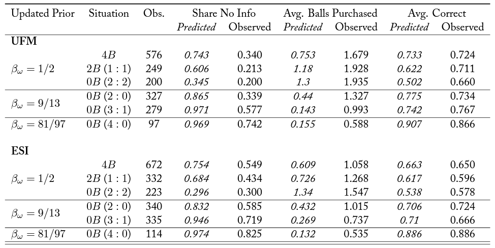
Table A.2 provides summary statistics of observed and predicted instances of “dropping out” (no information acquisition), amount of information acquired, and proportion of correct guesses by treatment and informational situation. Figure 1 presents, separately for the between- and the within-subject data, histograms of predicted and observed information acquisition by treatment and informational situation.²⁴ We observe that, across the informational situations, subjects purchase information more frequently than predicted and also purchase more signals than predicted.²⁵ At the same time, the data strongly support our main theoretical predictions. Thus, under asymmetric priors (i.e., $\beta _{\omega}=9/13$ in top row, a promise of future information induces greater information acquisition. This effect is strongest on the extensive margin: subjects drop out less and acquire at least some information more frequently. As predicted, the opposite is true in the knife-edge case ( $\beta _{\omega}=1/2$ ), where a promise of future information induces lower information acquisition.

Result 1.1 (extensive margin): With asymmetric priors ( $\beta _{\omega}=9/13$ , subjects are more likely to acquire a positive amount of information when free information is promised in the future ( $2B(2:0)$ ) than when no future information is offered ( $0B(3:1)$ ).

Support: The rate of information acquisition when free signals are promised after the purchasing decision is 0.535 (0.408) for the BSs (WSs) data and only 0.345 (0.313) when no free signals will be observed in the future. Using nonparametric tests, we reject the null that the probability of acquiring information in $2B(2:0)\leq 0B(3:1)$ using either the BSs data ( $U=2.702$ , $p=0.003$ ) or the WSs data $2B(2:0) \leq 0B(3:1)$ ( $z=2.475$ , $p=0.006$ ).

Our reduced-form estimates confirm the result. The top panel of figure 2 plots the relevant coefficients from a linear probability model. The full results of the regressions exploring the extensive margin are reported in table A.3.²⁶ We reject the null hypothesis using either a linear probability model (BSs: $p=0.004\$ , WSs: $p=0.015$ ) or a random effects logit model (BSs: $p=0.005$ , WSs: $p=0.009$ ). Using the linear probability model, we find that the probability of acquiring information increases by 8–17 percentage points (depending on whether we use BSs or WSs data) when future information is promised.

Having established that the promise of free signals increases the probability that a subject will purchase signals when priors are asymmetric, we turn to the intensive margin. Does the promise of free signals lead to more signals being purchased when priors are asymmetric?

Result 1.2 (intensive margin): When priors are asymmetric ( $\beta_{\omega}=9/13$ ), the promise of free information in the future ( $2B(2:0)$ ) leads subjects to acquire more information at cost, relative to the situation in which no free signals are promised in the future ( $0B(3:1$ ).

Support: In the BSs (WSs) data, subjects acquire $0.315$ ( $0.125$ ) more signals when future information is promised, on average. This is an increase of 37 percent (16 percent) compared to the situation when no future information is promised. Using nonparametric tests, we find that the number of signals acquired in situation $2B(2:0)$ is less than in situation $0B(3:1)$ . ). This is true for both the BSs data ( $U=1.680$ , $p=0.046$ ) and the WSs data ( $z=1.542$ , $p=0.062$ ), although the results are only marginally significant with the WSs data.

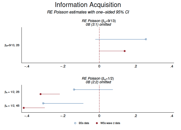
The reduced-form results obtained from our regressions are only marginally significant. This is true when estimating a random effects Poisson model (BSs: $p=0.065$ , WSs: $p=0.051$ ) or a random effects Tobit model (BSs: $p=0.058$ , WSs: $p=0.001$ ).²⁷The top panel of figure 3 presents coefficient plots for the random effects Poisson model. As the figure illustrates, although our results are only marginally significant, they have the predicted sign and are consistent across our two subsamples.

As discussed previously, exogenous variation in the realizations of the free signals that subjects observe before the information acquisition decision allow us to sample the relatively rare knife-edge case in which the updated prior implies indifference. Specifically, in situations $4B$ and $2B(1:1)$ subjects are promised free information in the future but have a prior of $\beta _{\omega}=1/2$ when purchasing signals. In situation $0B(2:2)$ (where the prior is also $\beta _{\omega}=1/2$ ), no additional free signals are forthcoming. Our model predicts that the promise of free signals in the future will reduce costly information acquisition in this case. This prediction is borne out in our data.

Result 2.1 (extensive margin): When $\beta _{\omega}=1/2$ , subjects are less likely to purchase signals when they know that they will observe free signals in the future. That is, the probability of purchasing signals is higher in $4B$ or $2B(1:1)$ than in $0B(2:2)$ .

Support: We reject the null hypothesis that the probability of acquiring any information is equal across the three relevant situations ( $\chi^{2} = 13.862$ , $p<0.001$ for BSs data; $Friedman = 195.2$ , $p<0.0001$ ; for WSs data). When restricting attention to pairwise comparisons, we reject the null that $4B \geq 0B(2:2)$ (BSs data: $U=-3.813$ , $p<0.0001$ ; WSs data: $z=-5.605$ , $p<0.0001$ ), that $2B(1:1) \geq 0B(2:2)$ (BSs data: $U=-1.680$ , $p=0.046$ ; WSs data: $z= -3.953$ , $p<0.0001$ ), and that $4B \geq 2B(1:1)$ (BSs data: $U=-2.2253$ , $p=0.013$ ; WSs data: $z=-3.341$ , $p<0.001$ ).

Our reduced-form models, reported in table A.3 and illustrated in the bottom panel of figure 2, also strongly support these results.²⁸

This result on the extensive margin is in line with the predictions of our model. However, it could be the case that the promise of free balls lowers the probability that a subject purchases signals while still increasing the quantity of signals purchased. As such, we turn to the intensive margin.

Result 2.2 (intensive margin): When $\beta _{\omega}=1/2$ , the promise of free signals to be observed after the information acquisition decision leads subjects to purchase fewer signals at cost. That is, fewer signals are purchased in $4B$ or $2B(1:1)$ than in $0B(2:2)$ .

Support: We reject the null hypothesis of equal information acquisition across the three relevant situations. Using the BSs data, this result is marginally significant ( $\chi^{2} = 4.752$ , $p= 0.093$ ), while it is highly significant ( $Friedman = 194.96$ , $p<0.0001$ ) when using the WSs data. When comparing situations with the largest difference in the number of free signals promised in the future ( $4B$ versus $0B(2:2)$ ), the results are highly significant. We reject the null that $4B\geq 0B(2:2)$ (BSs data: $U=-2.260$ , $p=0.0119$ ; WSs data: $-2.870$ , $p=0.002$ ). When there are only two additional signals promised in the future, the results have the predicted sign, but the significance of the nonparametric tests are inconsistent between the BSs and the WSs data. We can only reject the null that $2B(1:1) \geq 0B(2:2)$ using the WSs data (BSs data: $U=-1.194$ , $p=0.116$ ; WSs data: $z=-0.898$ , $p=0.019$ ). Similarly, for the null that $4B \geq 2B(1:1)$ , the results are only significant using the WSs data (BSs data: $U=-0.909$ , $p=0.182$ ; WSs data: $z=-2.431$ , $p<0.007$ ). This is driven by the higher level of statistical power available in the WSs data.

Our reduced-form results are consistent with the results of the nonparametric tests. Plots of the relevant coefficients are contained in the bottom panel of figure 3.²⁹ Note that the regression analysis consistently demonstrates that more signals are purchased in situation $4B$ than in situation $0B(2:2)$ . This is true for estimates obtained using a random effects Poisson model or a random effects Tobit model. However, when the comparison is less stark, we only reject the other null hypotheses ( $2B(1:1) \geq 0B(2:2)$ and $4B \geq 2B(1:1)$ ) using the WSs data.

In addition to the main hypotheses, our data support the prediction that promising free information in the future will not increase decision quality when priors are asymmetric. Despite differences in the amount of information acquired, the proportion of time the subjects choose the correct jar is no higher in $2B(2:0)$ than in $0B(3:1)$ .³⁰ However, in the knife-edge situations, where even small amounts of information are valuable, providing free information in the future is expected to slightly increase the predictive accuracy of guesses. We find support for this when comparing the most extreme situation with symmetric priors. That is, predictive accuracy is higher when four signals are promised relative to the case when no additional free signals are forthcoming ( $0B(2:2)$ versus $4B$ ).³¹

As demonstrated above, we find broad support for the theoretical predictions of our model. Most importantly, we find empirical support for the theoretically predicted ranking of information acquisition in the six situations we consider. However, our model fails to predict the observed level of information acquisition; our subjects consistently overacquire information. Such overacquisition is commonly observed in experimental settings, and our results are in line with those of Page and Siemroth (2017), who employ a similar environment to study information acquisition in asset markets. Similar overinvestment in information has been observed by Gretschko and Rajko (2015) in an auction context and by Chen and He (2021) and Hakimov et al. (2021), who study information acquisition in matching.

There is little consensus in the literature on the reasons for this rather consistent observation, and a number of possible explanations have been proposed. For example, Bhattacharya et al. (2017) and Meyer and Rentschler (2022) observe overinvestment in information in voting environments and consider quantal response equilibrium as a possible explanation. This, however, cannot explain our data as we focus on a decision-theoretic environment. Gretschko and Rajko (2015) hypothesize that overacquisition of information could be driven by regret avoidance.³² Chen and He (2021) consider several explanations and empirically assess the drivers of willingness to pay for information in a matching contest. They find that subjects’ willingness to pay increases in their beliefs about the willingness to pay of others and that curiosity also plays a significant role. Page and Siemroth (2017) find that information acquisition increases in subject endowments and decreases in risk aversion and experience in financial markets. They also find that observing inconclusive information leads to more information acquisition.

Conclusively determining the ability of most of these explanations to explain the overacquisition observed in our data would require additional research that would systematically vary aspects of the environment. This is beyond the scope of this paper, although we view it as a promising avenue for future research. However, since the second task of our experiment elicited the risk preferences of subjects, we can determine whether observed behavior can be explained by risk aversion. Unfortunately, the answer is negative. The difference between the predicted level of information acquisition of a risk-neutral agent and of an agent exhibiting the median level of risk aversion observed in our experiment is economically trivial.³³ Further, accounting for this median level of risk aversion often reduces the value of information. This demonstrates that risk aversion cannot explain our data on aggregate. Below, we will also demonstrate that observed risk aversion cannot explain the observed patterns in our data when accounting for individual heterogeneity in responses.

Individual Behavior

In this subsection we explore the heterogeneity of individual-level behavior. We begin with a descriptive analysis of individual heterogeneity and then focus on the WSs data to analyze individual-level behavior across treatments.

We start by checking whether individual subjects respond to experimental parameters in a manner consistent with our theoretical predictions. In the WSs data only 2/84 (2.38 percent) subjects never acquire any information in all 48 periods; 2/84 (2.38 percent) subjects buy at least one signal in all 48 periods. The median [10th, 90th percentile] individual buys at least one signal in 42.7 percent [10.4 percent, 81.3 percent] of the periods.³⁴ Most subjects also seem to have a downward-sloping demand for signals: for 70/84 (83.3 percent) of our subjects, we estimate a statistically significant negative effect of the cost on information acquisition (see figure B.5).³⁵

In a more subtle test of the theory, most subjects seem to understand the nonmonotonic value of signals, in which purchasing an even number of signals is never predicted. In fact, conditional on purchasing a positive number of signals, 11/84 (13.1 percent) of subjects always acquire an odd number of signals, whereas no subject chooses to always acquire an even number of signals. Again, conditioning on purchasing a positive number of signals, the median [10th, 90th percentile] subject acquires an odd number of signals 73.5 percent [52.1 percent, 100 percent] of the time. The number of subjects who, when purchasing, always purchase an odd number of signals more than double to 23/84 (27.4 percent) when excluding the first 12 periods, suggesting possible learning with experience.³⁶

For the rest of this subsection, we rely on the WSs data to examine heterogeneity in treatment effects across individuals. We focus on the case of the asymmetric prior where $\beta _{\omega}=9/13$ , and theory predicts that subjects will acquire more information if free information is promised in the future. For each individual $i$ , we compare the mean number of signals purchased across all periods in which subject $i$ was in situation $2B(2:0)$ to the mean number of signals purchased when subject $i$ was in subject $0B(3:1)$ .³⁷ We separately consider the comparison between the two knife-edge situations with a symmetric prior of $\beta _{\omega}=1/2$ : $2B(1:1)$ and $0B(2:2)$ .

To provide a meaningful comparison, for each subject, we compare the observed individual-level treatment effect to the predicted individual-level treatment effect, conditioning on the realized cost of information subjects actually faced in each period. We do this to account for the fact that subjects faced different costs across periods since the cost of signals is randomized in each period. For each subject, we directly compare the observed treatment effect to the predicted treatment effect, conditioning on the realized cost of information.

On average, pooling across all subjects, we predict a positive mean difference of 0.141: more information is predicted to be acquired when future free information is promised. However, there is considerable heterogeneity at the individual level: predicted difference in means is positive for 46 (54.8 percent) subjects, 0 for 17 (20.2 percent), and negative for 21 (25 percent). (To reiterate, this happens because some subjects faced lower costs in $0B(3:1)$ than in $2B(2:0$ ).)

Figure 4 illustrates (for each of the 84 subjects from the wave 2 sessions) the observed difference in individual-level information acquisition when $\beta_{\omega}=9/13$ . Solid circles indicate the average number of signals purchased in situation $2B(2:0)$ less the average number of signals purchased in situation $0B(3:1)$ . Empty diamonds indicate the respective predicted difference. For comparison, figure 5 presents the same for the knife-edge case of $\beta_{\omega}=1/2$ . The white $x$ s ( $+$ s) denote the two subjects who never (always) acquire any signals.

In both of the preceding figures, the coloring of the solid circles denotes the relationship between the observed treatment effect and the predicted treatment effect. Black circles denote individuals whose observed difference in mean behavior across treatments has (weakly) the same sign as the predicted difference. Red circles denote individuals where the observed and predicted differences have the opposite sign. The vertical lines connecting the circle and diamonds indicate the distance between the observed and predicted differences. Red lines denote instances in which the observed difference in mean behavior across treatments is less than the predicted difference. For subjects whose observed difference has the same sign as the predicted difference (black solid dots), the red line indicates that they underresponded to the theoretically predicted treatment difference. Gray lines indicate instances in which the observed difference has the same sign as the predicted difference but the magnitude is larger than predicted.

Of note is the fact that when $\beta_{\omega}=9/13$ , the individual-level treatment effect fails to match the sign of the predicted effect for only 17/84 of subjects. Further, when $\beta_{\omega}=1/2$ , only 27/84 subjects fail to match the sign of the observed and the predicted difference. That is to say, while there is significant heterogeneity in individual-level treatment effects, our results are not driven by a small number of outliers. Rather, the behavior of the majority of subjects are qualitatively in line with the theoretical predictions.

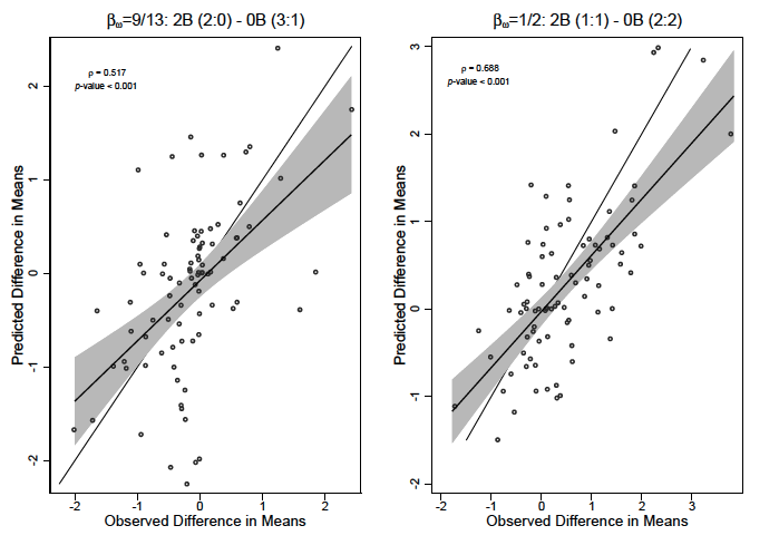
We next explore how well the individual-level treatment effects correlate with the predicted individual-level treatment effects. Figure 6 presents a scatter plot and a linear fit (with the associated 95 percent confidence interval) of predicted individual-level treatment differences and the predicted individual-level treatment differences. The left panel illustrates situations where $\beta_{\omega}=9/13$ , and the right panel illustrates situations in which $\beta_{\omega}=1/2$ . There is a strong, positive correlation both when $\beta_{\omega}=9/13$ ( $\rho=0.517$ , $p<0.001$ ) and when $\beta_{\omega}=1/2$ ( $\rho=0.688$ , $p<0.001$ ).

These results are further backed by the regression analysis reported in tables A.6 and A.7. The tables report ordinary least squares (OLS) estimates of the individual-level differences in behavior across treatments for $\beta_{\omega} =9/13: 2B (2:0) - 0B (3:1)$ and $\beta_{\omega} =1/2: 2B (1:1) - 0B (2:2)$ , respectively. In both tables, the dependent variable in columns 1–2 (4–5) is individual differences in mean (median) information acquisition across situations. The dependent variable in column 3 (6) is the individual observed deviation from predictions. Column 2 (4) shows that the predicted difference in means (medians) is positive and statistically significantly correlated with the observed difference. The difference in means, however, is smaller than (and statistically significantly different from) one. For the difference in medians (column 4), we cannot reject the null hypothesis that the coefficient is equal to one.

Regarding individual-level characteristics that may correlate with treatment effects, we observe that the only robust and consistent difference is related to the measured risk preferences, as measured by the number of safe options the subject chose in the risk elicitation task.³⁸ In particular, we find that treatment differences are smaller for those who are more risk averse. However, it is important to note that the magnitude of these coefficients is small.

The main takeaway is that we observe a strong and positive correlation between individual-level observed and predicted difference in means (medians). Thus, despite individual heterogeneity, we find that a large majority of subjects exhibit behavior that differs across treatments in the same direction as the theoretical predictions and that individual differences in behavior across treatments are strongly correlated with the theoretical predictions.

Discussion and Further Research

We present results of a laboratory experiment on the impact a promise of future information may exert on individual information acquisition effort. We observe that offering future information encourages greater costly information acquisition. Furthermore, when we explore the knife-edge case of symmetric priors, we observe (as predicted) that the promise of future information reverses this result. At the aggregate level, the differences across treatments are more pronounced on the extensive than on the intensive margin: a promise of delayed information makes the agents less likely to choose not to acquire any information at all. As predicted by the model, information acquired in this manner is ex post useless: the quality of the overall decision-making is unaffected.

The aggregate results are not driven by a few subjects. When focusing on individual-level treatment differences using the within-subject variation, we find that behavioral support for the theory is widespread. Out of the 80 subjects who exhibit responsiveness to experimental parameters in their information acquisition decisions, about 65 percent show a difference in information acquisition across the laboratory environments going in the same direction as the theoretical prediction. Furthermore, we find a strong correlation between the observed and predicted differences in mean information acquisition decisions across treatments. Thus, we observe strong evidence to support the theory, both at the aggregate and the individual level. The effect we identify appears to be an important, previously unobserved feature of costly attention environments and may therefore be used to identify rational inattention in the field.

Though a promise of free information may create incentives for costly information acquisition that would not exist otherwise, it does not improve the quality of individual decisions, nor the welfare of the decisionmaker. This confirms the theoretical prediction that follows straightforwardly from Blackwell (1962).³⁹ However, in group settings, such as juries or committees, if we can use the promise of future information to induce additional information acquisition effort by individuals, we may expect it to have spillovers on others. In fact, this reasoning may be behind the typical prohibition for jurors to talk about the evidence they listen to during a trial until all evidence is presented. In Hannaford et al. (2000), the authors show intriguing evidence of increased drop out by jurors in a field experiment in which this prohibition was relaxed, lending support for the hypothesis we have just laid out. Consequently, in terms of institutional design, delay in information provision may be sufficient to discourage “informational dropout,” situations in which agents choose to forgo attentional effort and make decisions based entirely on their prior beliefs. It may also be a useful tool in experimental design as it could be used to avoid excessive dropout by subjects that has been observed in some previous experimental studies (Elbittar et al., 2020).

Finally, this study poses some questions to the important literature that evaluates the impact of free information provision and suggests that a more rigorous framework is needed. Since the information provided in most studies cannot be anticipated at the moment of making information acquisition decisions, it would seem that the impact of information provision may sometimes be ambiguous. Thus, a good applied information provision design should take into account the nonconcavity in the value of information, make explicit the underlying assumptions behind the baseline priors, and incorporate the impact of established biases (such as, e.g., base rate neglect). Our paper aims to provide a laboratory contribution to answering at least some of these questions.

Tables

Table 1.

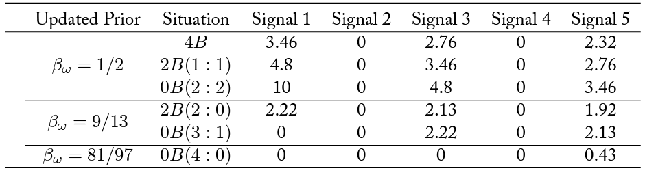
Notes: The table shows the marginal value of purchasing a signal in percentages of the prize value at the moment of information acquisition. To understand the numbers in this table, consider the marginal value of going from one to three signals having previously observed two red signals. Purchasing the extra two signals could change the agent’s choice only if either two or all three of the signals she is already set to observe (the two free signals and the one the agent has already decided to purchase) would turn out to be blue. In the former case, the agent would change her choice if she observes two blue signals. In the latter case, she would change her choice if she observes two red signals. Having observed two red signals, the agent’s current prior belief that the jar is red is $\beta =9/13$ . Combining the ex ante value of observing two blue signals after one red and two blue, and two red signals after three blue, and substituting the signal strength $p=0.6$ , we obtain $3\left(1-\beta \right) \left( 1-p\right) p^{4}-3\beta p\left( 1-p\right) ^{4}+\beta \left( 1-p\right) ^{3}p^{2}-\left( 1-\beta \right) p^{3}\left( 1-p\right)^{2}={2.13}$ .

Table 2.

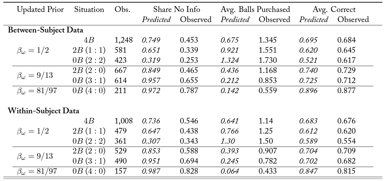
Notes: The table shows summary statistics of predicted and observed actions for between- and within-subject data, according to the updated priors generated by the informational situation. “Obs.” denotes the number of observations collected in each informational situation. “Share No Info” is the relative number of instances where no information was purchased. “Avg. Balls Purchased” denotes the unconditional number of signals purchased. “Avg. Correct” is the share of correct guesses.

Figures

Figure 1. Histogram of Predicted and Observed Balls Purchased by Treatment and Informational Case.

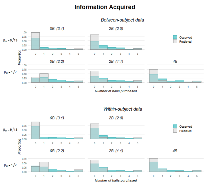
The top panel shows between-subject (BSs) data, and the bottom panel shows within-subject (WSs) data. The top row of each panel shows situations where $\beta_{\omega}=9/13$ , and the bottom row of each panel shows the rare knife-edge case of indifference ( $\beta_{\omega}=1/2$ ).

Figure 2. Coefficient Plots for Linear Probability Estimates of the Effects of Promising Future Information on the Decision to Acquire Information (Extensive Margin).

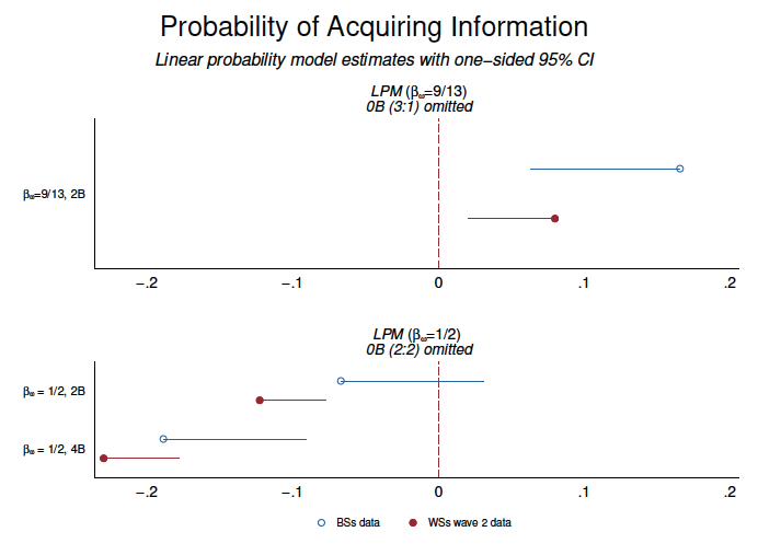
The figures shows results from joint estimates using all informational cases. The top panel ( $\beta_{\omega}=9/13$ ) presents estimates of promising two balls ( $2B$ ) after information acquisition relative to the omitted category of no information $\0B$ in the future. The bottom panel presents estimates of promising two ( $2B$ ) and four ( $4B$ ) balls after information acquisition relative to the omitted category of no information ( $0B$ ) in the future for the rare knife-edge case of indifference ( $\beta_{\omega}=1/2$ ).

Figure 3. Coefficient Plots for Random Effects Poisson Model Estimates of the Effects of Promising Future Information on the Decision of the Number of Signals to Acquire (Intensive Margin).

The figures shows results from joint estimates using all informational cases. The top panel ( $\beta_{\omega}=9/13$ ) presents estimates of promising two balls ( $2B$ ) after information acquisition relative to the omitted category of no information ( $0B$ ) in the future. The bottom panel presents estimates of promising two ( $2B$ ) and four ( $4B$ ) balls after information acquisition relative to the omitted category of no information ( $0B$ ) in the future for the rare knife-edge case of indifference ( $\beta_{\omega}=1/2$ ).

Figure 4. Across-Treatment Individual Difference in Mean Information Acquisition (2B–0B) Observed and Predicted for $\beta _{\omega}=9/13$ .

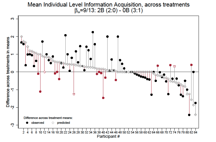
Participants are sorted by the predicted difference in means, from highest to lowest.

Figure 5. Across-Treatment Individual Difference in Mean Information Acquisition (2B–0B), Observed and Predicted for $\beta _{\omega}=1/2$ .

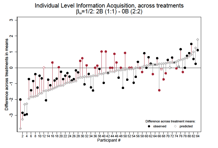
Participants are sorted by the predicted difference in means, from lowest to highest.

Figure 6. Correlation between Observed and Predicted Individual Differences across Treatments in Mean Information Acquisition across Treatments, for Different Updated Priors.

Additional Tables

Table A.1. Summary Statistics by Treatment

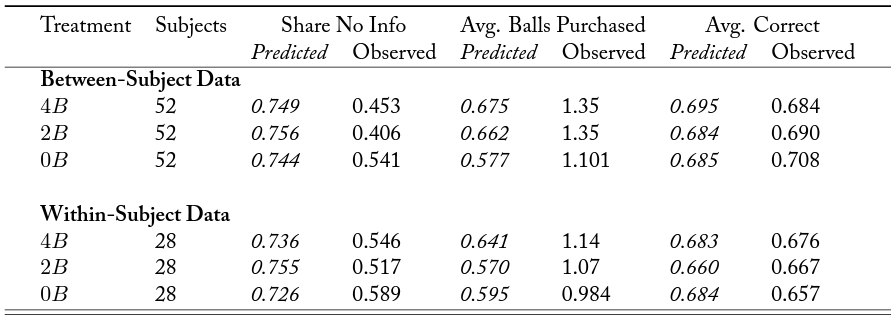
Table A.2. Summary Statistics for Main Task (BSs Data) by Wave

Notes: The table shows summary statistics by the treatment and information scenarios for the main task (24 periods) of each wave, according to the updated priors generated by the informational case (situation). “Obs.” denotes the number of observations collected in each informational case. “Share No Info” is the relative number of instances where no information was acquired. “Avg. Balls Purchased” denotes the unconditional number of balls purchased. “Avg. Correct” is the share of instances of correct state-of-theworld predictions (color of jar guesses).

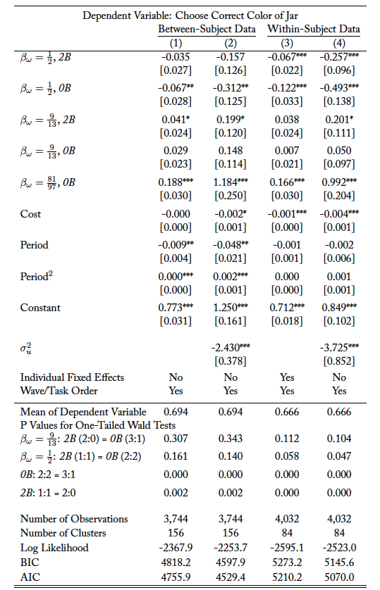
Table A.3. Information Acquisition: Extensive Margin

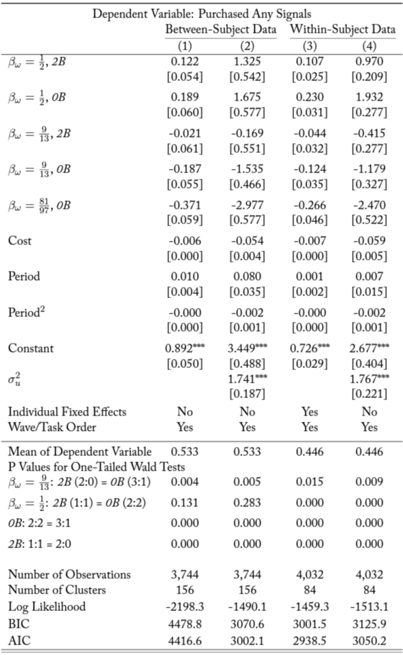
Notes: The table shows linear probability model (1 and 3) and random effects logit model (2 and 4) estimates of the probability of information acquisition. Estimates using between- (within-) subject data are reported in columns 1 and 2 (3 and 4). Robust standard errors are clustered at the individual level in brackets. The omitted treatment variable is baseline treatment $4B$ ( $\beta _{\omega}=\frac{1}{2}$ ): no free information before decision to acquire information.

Table A.4. Information Acquisition: Intensive Margin

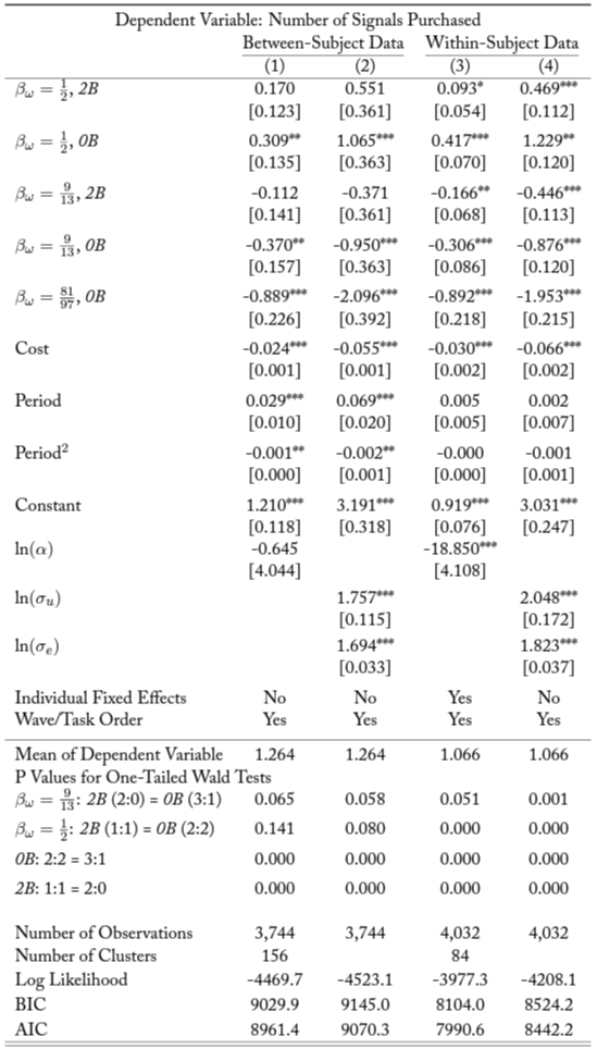
Notes: The table shows random effects Poisson model (1 and 3) and random effects Tobit model (2 and 4) estimates of the amount of information acquired (number of balls purchased). Estimates using between- (within-) subject data reported in columns 1 and 2 (3 and 4). Standard errors (clustered at the individual level for specifications 1 and 3) in brackets. Omitted treatment variable is baseline treatment $4B$ ( $\beta _{\omega}=\frac{1}{2}$ ): no free information before decision to acquire information.

Table A.5. Correct Choice

Notes: The table shows linear probability model (1 and 3) and random effects logit model (2 and 4) estimates of the probability of correctly predicting the state of world (guessing the color of the jar). Estimates using between- (within-) subject data are reported in columns 1 and 2 (3 and 4). Robust standard errors are clustered at the individual level in brackets. The omitted treatment variable is baseline treatment $4B$ ( $\beta _{\omega}=\frac{1}{2}$ ): no free information before decision to acquire information.

Table A.6. Determinants of Individual-Level Differences in Mean/Median Information Acquisition across Treatments for $\beta_\omega=9 / 13: 2 B(2: 0)-0 B(3: 1)$

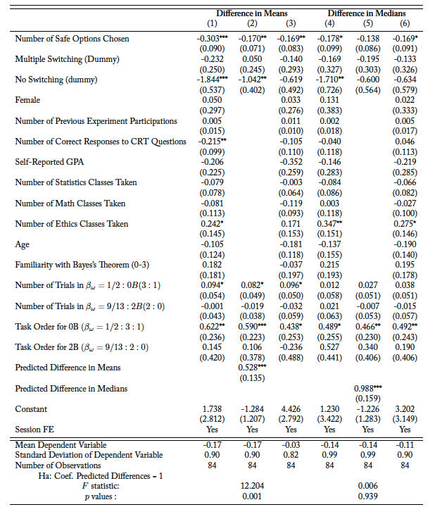
Notes: The table shows OLS estimates of the individual-level behavior across treatments for $\beta_{\omega} =9/13: 2B (2:0) - 0B (3:1)$ . The dependent variable in columns 1–2 (4–5) is individual differences in mean (median) information acquisition across treatments. The dependent variable in column 3 (6) is the individual observed deviation from predictions in differences in mean (median) information acquisition across treatments. Robust standard errors are in parentheses. * p $<$ 0.10, ** p $<$ 0.05, *** p $<$ 0.01

Table A.7. Determinants of Individual-Level Differences in Mean/Median Information Acquisition across Treatments for $\beta_\omega=1 / 2: 2 B(1: 1)-0 B(2: 2)$

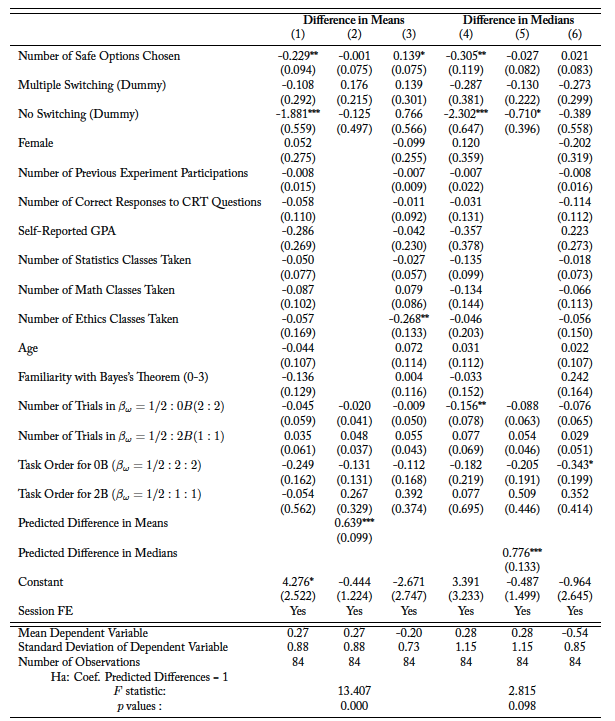
Notes: The table shows OLS estimates of the individual-level behavior across treatments for $\beta_{\omega} =1/2: 2B (1:1) - 0B (2:2)$ . The dependent variable in columns 1–2 (4–5) is individual differences in mean (median) information acquisition across treatments. The dependent variable in column 3 (6) is the individual observed deviation from predictions in differences in mean (median) information acquisition across treatments. Robust standard errors are in parentheses. * p $<$ 0.10, ** p $<$ 0.05, *** p $<$ 0.01

Additional Figures

Figure B.1. Coefficient Plots of Linear Probability Models Estimating the Probability of Purchasing Any Signals with Estimates Obtained Separately for Each Sample

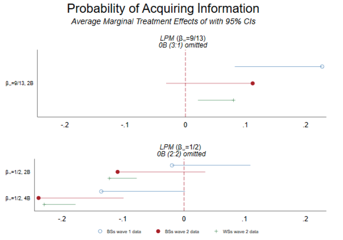
Figure B.2. Coefficient Plots of Poisson Models Estimating the Number of Purchased Signals with Estimates Obtained Separately for Each Sample

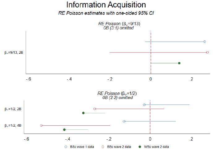
Figure B.3. CDF of Information Purchased by Individuals during Last 12 Periods, by Treatment and Information Scenario for BSs

Figure B.4. CDF of Information Purchased by Individuals during Last 12 Periods, by Treatment and Information Scenario for WSs

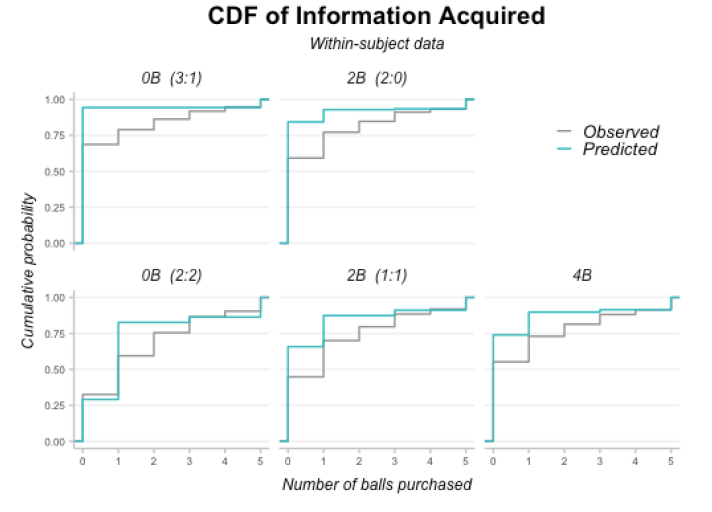
Figure B.5. Individual Estimates of the Effect of Cost on Information Acquisition Decisions Using within-Subject Data (Chapman-ESI Sample).

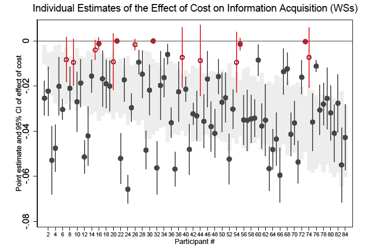
The figure plots point estimates with 95 percent confidence intervals. The shaded area corresponds to 95 percent confidence intervals for the predicted effect of cost on information acquisition under risk neutrality.

Figure B.6. Individual Estimates of the Effect of Cost on Information Acquisition Decisions Using between-Subject Data from Wave 1 (UFM Sample).

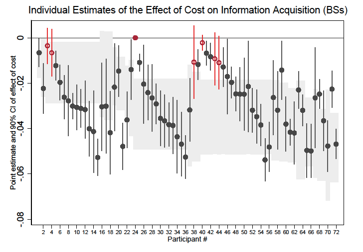
The figure plots point estimates with 90 percent confidence intervals. The shaded area corresponds to 90 percent confidence intervals for the predicted effect of cost on information acquisition under risk neutrality.

Appendix C: Sample Instructions

References

Allcott, Hunt and Dmitry Taubinsky, “Evaluating behaviorally motivated policy: Experimental evidence from the lightbulb market,” American Economic Review, 2015, 105 (8), 2501–2538.

Battaglini, Marco, Rebecca B. Morton, and Thomas R. Palfrey, “The swing voter’s curse in the laboratory,” Review of Economic Studies, 2010, 77 (1), 61–89.

Bernheim, B. Douglas and Dmitry Taubinsky, “Behavioral Public Economics,” in “Handbook of Behavioral Economics,” Vol. 1, Elsevier B.V., 2018, chapter 5, pp. 381–516.

Bhargava, Saurabh, George Loewenstein, and Justin Sydnor, “Choose to lose: Health plan choices from a menu with dominated options,” The Quarterly Journal of Economics, 2017, 132 (3), 1319–1372.

Bhattacharya, Sourav, John Duffy, and Sun Tak Kim, “Voting with endogenous information acquisition: Experimental evidence,” Games and Economic Behavior, 2017, 102, 316–338.

Blackwell, David, “Equivalent Comparisons of Experiments,” The Annals of Mathematical Statistics, 1962, 33 (2), 719–726.

Bollinger, Bryan, Phillip Leslie, and Alan Sorensen, “Calorie posting in chain restaurants,” American Economic Journal: Economic Policy, 2011, 3 (1), 91–128.

Caplin, Andrew and Daniel Martin, “A testable theory of imperfect perception,” Economic Journal, 2015, 125 (582), 184–202.

and , “Framing as Information Design,” 2018.

and Mark Dean, “Revealed preference, rational inattention, and costly information acquisition,” American Economic Review, 2015, 105 (7), 2183–2203.

Chade, Hector and Edward E. Schlee, “Another look at the Radner-Stiglitz nonconcavity in the value of information,” Journal of Economic Theory, 2002, 107 (2), 421–452.

Chaloupka, Frank J., Kenneth E. Warner, Daron Acemoğlu, Jonathan Gruber, Fritz Laux, Wendy Max, Joseph Newhouse, Thomas Schelling, and Jody Sindelar, “An evaluation of the FDA’s analysis of the costs and benefits of the graphic warning label regulation,” Tobacco Control, 2015, 24 (2), 112–119.

Chen, Yan and Yinghua He, “Information acquisition and provision in school choice: an experimental study,” Journal of Economic Theory, 2021, p. 105345.

Dean, Mark and Nathaniel Neligh, “Experimental Tests of Rational Inattention,” Working Paper, 2017, ( June), 1–55.

Elbittar, Alexander, Andrei Gomberg, César Martinelli, and Thomas R Palfrey, “Ignorance and bias in collective decisions,” Journal of Economic Behavior and Organization, 2020, 174, 332–359.

Feltovich, Nick, “Nonparametric tests of differences in medians: comparison of the Wilcoxon–Mann–Whitney and robust rank-order tests,” Experimental Economics, 2003, 6 (3), 273–297.

Fischbacher, Urs, “z-Tree: Zurich toolbox for ready-made economic experiments,” Experimental economics, 2007, 10 (2), 171–178.

Fligner, Michael A and George E Policello, “Robust rank procedures for the Behrens-Fisher problem,” Journal of the American Statistical Association, 1981, 76 (373), 162–168.

Frederick, Shane, “Cognitive reflection and decision making,” Journal of Economic perspectives, 2005, 19 (4), 25–42.

Golman, Russell, David Hagmann, and George Loewenstein, “Information avoidance,” Journal of Economic Literature, 2017, 55 (1), 96–135.

Gretschko, Vitali and Alexander Rajko, “Excess information acquisition in auctions,” Experimental Economics, 2015, 18 (3), 335–355.

Grosser, Jens and Michael Seebauer, “The curse of uninformed voting: An experimental study,” Games and Economic Behavior, 2016, 97, 205–226.

Guarnaschelli, Serena, Richard D. Mckelvey, and Thomas R. Palfrey, “An Experimental Study of Jury Decision Rules,” American Political Science Review, 2018, 94 (2), 407–423.

Hakimov, Rustamdjan, Dorothea Kübler, and Siqi Pan, “Costly information acquisition in centralized matching markets,” 2021.

Hannaford, Paula L., Valerie P. Hans, and G. Thomas Munsterman, “Permitting jury discussions during trial: Impact of the Arizona Reform.,” Law and Human Behavior, 2000, 24 (3), 359–382.

Kanazawa, Satoshi, “What do we do with the WEIRD problem?,” Evolutionary Behavioral Sciences, 2020, 14 (4), 342.

Larreguy, Horacio, John Marshall, and James M Snyder, “Publicizing malfeasance: When the local media structure facilitates electoral accountability in Mexico,” The Economic Journal, 2020.

León, Gianmarco, “Turnout, political preferences and information: Experimental evidence from Peru,” Journal of Development Economics, 2017, 127 (December 2016), 56–71.

Meyer, Jacob and Lucas Rentschler, “Abstention and informedness in nonpartisan elections,” Working Paper, 2022.

Page, Lionel and Christoph Siemroth, “An experimental analysis of information acquisition in prediction markets,” Games and Economic Behavior, 2017, 101, 354–378.

Radner, Roy and Joseph Stiglitz, “A Nonconcavity in the Value of Information,” in M. Boyer and R.E. Kihlstrom, eds., Bayesian models in economic theory, Elsevier, 1984, chapter 3, pp. 33–52.

Does Free Information Provision Crowd Out Costly Information Acquisition? It’s a Matter of Timing

Executive Summary

Resources

Focuses

Introduction

Theory

Experimental Design

Experimental Tasks and Protocols

Data and Empirical Strategy

Results

Individual Behavior

Discussion and Further Research

Tables

Figures

Additional Tables

Additional Figures

Appendix C: Sample Instructions

References

Executive Summary

Resources

Related Publications

Related News

Related Blogs

Focuses

Introduction

Theory

Experimental Design

Experimental Tasks and Protocols

Data and Empirical Strategy

Results

Individual Behavior

Discussion and Further Research

Tables

Figures

Additional Tables

Additional Figures

Appendix C: Sample Instructions

References