
1 Introduction
Twenty-five percent of participants in the United States workforce require an occupational license, which is greater than the percentage of workers directly impacted by unions or the minimum wage (U.S. Bureau of Labor Statistics 2016). Occupational licensing is the mechanism of imposing minimum requirements to work within a specific job classification, and these requirements generally differ at the state-level. An individual attempting to obtain an occupational license will incur costs in the form of fees, examinations, and days required to complete education and experience mandates. Obtaining an occupational license for employees, or paying a wage premium for licensed workers, constitutes a significant cost consideration for firms. These costs may influence whether a business enters into a market or hires employees. Understanding the relationship between occupational licensing costs and firm decisions have important policy implications for how a state encourages business development and employment.
There is a growing body of literature focusing on the costs and benefits of occupational licensing. Proponents cite the benefits of occupational licensing as the protection of public health, consumer safety, and higher wages for employees (Kleiner & Krueger, 2010). Opponents of the current form of regulations claim these benefits are outweighed by the harm caused from increased prices for consumers and reduced aggregate economic mobility (Cox & Foster, 1990; Carroll & Gaston, 1981; Kleiner & Krueger, 2010; Meehan et al., 2017). Wage premiums for license-holding employees in heavily regulated industries tend to be larger in states with steeper occupational licensing costs (Akerlof, 1970; Shapiro, 1986; Kleiner & Krueger, 2013; Timmons & Thornton, 2008). The effects of these wage premiums on firm location and hiring decisions, however, has yet to be investigated.
The purpose of this study is to analyze how occupational licensing regulations influence entry and employment decisions of firms by analyzing the patterns exhibited by businesses that are located near state borders. In this study, I analyze the likelihood that a firm will enter the market from a specific side of a state border, given the differences in licensing costs, using a series of logistical functions. To observe differences in firm employment patterns over state borders I utilize a geographic regression discontinuity design to determine if there is a systematic difference in the average number of employees per firm, in bins of distance from the state border, between high- and low-cost states. Finally, to further substantiate claims of causal differences in average firm employment, I perform a non-temporal difference-indifference analysis between a variety of firm-industry pairs that perform similar business functions. In each pair of firms, one firm generally employs workers that require occupational licensing in most states, while the other does not. The purpose of this approach is to confirm that changes in firm entry decisions are influenced by occupational licensing costs and not by other state or industry trends.
Previous studies focus on the effects of occupational licensing regulations on employees in the form of wage premiums and on consumers in the form of price and quality changes for goods and services. To my knowledge, my model is one of the first spatial models developed for understanding the relationship between firm density and occupational licensing costs near state borders. My empirical methodology provides an analytical explanation of firm entry decisions and the causal effects of occupational licensing costs on firm employment near state borders. In doing so, I explain how these regulations affect decisions and preferences of firms, which can have widespread effects on public policy and welfare.
I find an increased probability of firms entering on the cheaper side of a state border pair as occupational licensing cost differences increase. The magnitude of these correlations is larger for businesses in laborintensive industries. Using a geographic regression discontinuity framework, I find negative point estimations for differences in average firm employment in high-cost states relative to low-cost states. There are substantial discontinuities in employment around state borders, which persist even after accounting for population and geographic attributes. Comparing pairs of industries that differ only in their occupational licensing requirements, I find that there is a substantial negative effect on average firm employment for licensed firms in high-cost states that are not present for unlicensed firms.
The paper will proceed as follows: Section 2 provides an overview of the relevant literature. Section 3 provides details on the data that will be used for analysis. Section 4 develops the empirical models that will be used to analyze the three different specifications of firm-levels. Section 5 presents the empirical results of the models. Section 6 concludes and discusses policy relevance.
2 Literature Review
Governments introduced occupational licensing to help consumers understand and judge the quality of professional services and to signal to consumers that a license holder is qualified to provide the good or service (Law & Kim, 2005; Arrow, 1971). Technological advances and increased professional specialization had made it increasingly difficult for individuals to judge differences between service providers. For most industries, an individual state chooses whether an occupation is subject to occupational licensing; likewise, states choose the fees, education, and experience requirements to meet the standards for that job. These requirements often differ drastically between states and can increase the cost of conducting business for firms (van Stel et al., 2007). Researchers have focused on occupational licensing, even though there are alternatives (e.g., certifications and output monitoring) since these alternatives are far less prevalent in most industries (Cox & Foster, 1990). Within the United States, the proportion of jobs that require some sort of occupational license has grown from approximately 4 percent of the workforce in the early 1950s to 25 percent of the workforce in 2008 (U.S. Bureau of Labor Statistics, 2016).
In recent decades, a substantial amount of literature has centered on analyzing the costs and benefits of occupational licensing for either workers or consumers. Workers who are subject to occupational licensing often benefit from wage premiums; however, at the economy level, some studies find these licenses may have reduced aggregate economic mobility (Kleiner & Park, 2010; Kleiner & Krueger, 2010, 2013; Meehan et al., 2017). Consumers are subject to substantial changes in cost through price effects. These 5 price effects, in theory, represent payments for increased public health, safety, and quality of goods and services (Arrow, 1971).
Blair and Chung (2018) use a boundary discontinuity design to measure the effects of licensing on occupational choice and find that it can reduce the equilibrium labor supply by an average of 17–27 percent. Gittleman et al. (2018) find that individuals who invested into human capital and obtained a license earn higher pay, are more likely to be employed within their field, and also have a higher probability of access to employer-sponsored healthcare. Survey data find that having a government-issued occupational license is associated with an approximate 11 percent differential in increased wages after controlling for human capital and other observables (Kleiner & Vorotnikov, 2017). Evidence of wage premiums has also been documented within individual industries including but not limited to the following: radio technologists, construction workers, dental hygienists, childcare professionals, opticians, and veterinary technicians (Timmons & Thornton, 2008; Kleiner & Park, 2010; Perloff, 1980; Guis, 2016).
These wage premiums are designed to incentivize education and training, improve public health and safety, and increase overall quality of goods and services (Akerlof, 1970; Shapiro, 1986). Yet studies on the quality benefits of occupational licensing in the United States have generally found mixed effects on the quality of goods and services (Kleiner & Kudrle, 2000; Carroll & Gaston, 1981; Angrist & Gyruan, 2008; Kane et al., 2008; Maurizi, 1980). Though the quality effects of occupational licensing restrictions are mixed, consumers are also affected by price changes. Conrad and Sheldon (1982) find that restrictions on the number of firm branches and dental assistant procedures led to a 4 percent increase in consumer prices. Kleiner and Kudrle (2000) find that states saw substantial increases in prices when restrictions were increased for dental services. In similar studies for optometry, Bond et al. (1980) and Haas-Wilson (1986) find higher prices of eye exams and eyeglasses in states with restrictions on optometrists’ commercial practices. These increased prices may also result in consumers eventually lowering their demand over time as they substitute away from the service (Adams et al., 2002; Kleiner, 2017).
The wage premium for licensed employees can represent an additional cost for firms who wish to enter or remain in a market. The costs to firms cannot always be offset with increases in prices because they may harm demand over time. To avoid these costs, firms may self-select into areas where they have the lowest cost to open and conduct business. Since occupational licensing costs are determined at the state level, there can be large differences in cost on either side of a state border, even if the local physical attributes of the location are the same. This study attempts to shift the focus away from consumers and employees and instead investigates how occupational licensing affects business decisions, including where a firm operates and how many employees it hires.
Zapletal (2018) is the closest study to my own, as it focuses on the location decisions of businesses, though it focuses specifically on personal care industries. Zapletal finds that license restrictiveness affected businesses’ decisions to enter and exit the market but not their overall quality, services, or prices for 6 cosmetology-related services. Complementary studies have found that occupational licensing also influences the mobility and migration of workers and firms (Holen, 1965; Johnson & Kleiner, 2017; Pashigian, 1979). Some studies have also found that occupational licensing can influence the entry decision of entrepreneurs, especially immigrant entrepreneurs (Federman et al., 2006; Slivinski, 2017). In this study, I am interested in whether these effects influence the likelihood that a business will enter the market in a given location, with the consideration that there are additional costs in the form of wage premiums or payments for workers to maintain licenses. Firms choosing locations for their businesses must also consider that the labor force in these regulated industries is less mobile between states.
3 Data
3.1 Occupational Licensing
State requirements for occupational licensing were acquired from the Institute for Justice License to Work (LTW) 2017 update. The LTW distinguishes between reported occupations that require an occupational license and those that require only a certification. An occupational license requirement is when government authorization is required to legally perform the services of that occupation. For example, an Emergency Medical Technician (EMT) requires an occupational license in all 50 states and the District of Columbia; this means that a license must be obtained to work as an EMT in any capacity. Consequently, a non-licensed individual can not be hired for an EMT position. Certifications differ in that, while they also signal competency in a field, they are not required to perform a specific service. For example, a bartender may obtain a certification in 38 states but can still be a bartender without the certification. In this case the EMT data would be included in LTW report data for all states, but the bartender would not be considered under the burden of an occupational license in the certification-only states. This report measures the regulatory burden associated with 102 occupations regulated in all 50 states and the District of Columbia. Information on each regulated occupation includes fees, examinations, and the calendar days necessary to complete mandatory education and experience requirements. Though this report does not cover every occupation subject to an occupational license, it is currently the largest available database of licenses, and these measures can serve to provide a foundation for determining a state’s regulatory environment and stringency.
Tables 3 and 4 contain summary statistics for the state-level variables and cross-differenced state-level variables, respectively. To measure the regulatory environment of a state, simple averages are taken across occupations of the monetary fees and number of calendar days required to complete mandatory education and training for obtaining a license. These variables allow for the comparison of differences in regulatory environments between states. For the United States, Nevada is the most expensive state in terms of monetary fees, with $704 being the average cost of an occupational license. The least expensive is Nebraska, where the average cost for a license is $76. Across the states the mean is $268.14, with a standard deviation of $113.77. In regard to calendar days required to complete mandatory education and training, Pennsylvania has the shortest number of average days required at 117.2 days. Hawaii, in comparison, has the highest average estimated days required to complete mandatory education and training, at 988 days. For the United States, the mean is 373.7 days, with a standard deviation of 199.5 days. Both variables are approximately standard normal in their distribution.
3.2 Firm-Level Characteristics
I obtained data on firm characteristics and locations through large-scale web scraping from a popular sales lead company, Reference USA, during April 2017. These data are collected at the firm level, as opposed to earlier studies that used establishment data aggregated to the zip code or county level. Collected variables include the exact longitude and latitude of the firm location, SIC and NAICS codes at the sixdigit level, employee and sales estimations, credit ratings, etc. Figure 1 contains a map of the exact locations for the 3,174,670 firms in my sample. The firms contained in this data set were established between 1994 and 2016 and are located within the continental United States. This study is limited to companies that were established in or after 1994 because the focus of the study is on companies from the internet age. The internet drastically changed the ability of companies to conduct sales and services at a distance, which affects business entry and location decisions.
Figure 1. Map of All Firm Locations
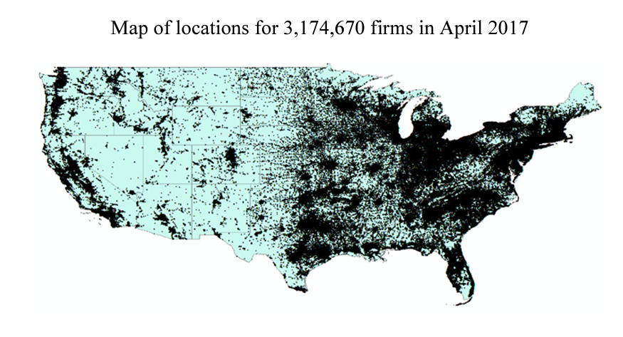
The data used in this study contain information on the industry classification of each firm. Table 1 contains summary statistics for the number of firm observations within nine major industry classifications. This information allows for the same interactions to be analyzed for subsets of data to determine if occupational licensing burdens have a larger effect within specific industries. This table also contains the average number of employees per firm location for each of the industry sectors, with an overall average of 8.14. The smallest industry—in terms of total number of businesses, with 19,188 firms representing approximately 0.60 percent of the total firm data—is the Public Administration industry. The largest industry, representing 46.01 percent of the data with 1,460,624 firms, is the Services sector. These 8 industries are defined at the two-digit NAICS level, though future research may be determined at more specific four- and six-digit NAICS levels as well.
3.3 Similar Industry Matches
To address possible endogeneity concerns for the relationship between occupational licensing and average firm employment, I identify pairs of firms that perform similar economic functions but that differ in whether they generally hire licensed employees. This is often difficult because in most cases similar business types fall under the same six-digit NAICS code. Since data are unavailable for the occupational licensing of every individual firm employee, generalizations must be made to attempt to compare industries. Though these matches are not perfect substitutes for each other, they provide insight into whether industries that are known to hire workers with occupational licenses have significant average employment differences, by comparing them to industries that should be unaffected. Table 2 shows the six business pairs that this study will compare in the empirical analysis.
Match Type (1), transportation, compares Taxi Services (NAICS 485310) with Other Transit and Ground Passenger Transport (NAICS 485999). Taxi drivers are required to maintain special occupational licenses in 16 states and most major cities. Since many states require occupational licenses for taxi drivers, this study identifies Taxi Services as having generally licensed employees. Other Transit and Ground Passenger Transport includes a wide variety of passenger transit, including shuttle services and van pools. Shuttle and van operators are often not required to have any additional occupational licensing, so this study defines these firms as having unlicensed employees.
Match Type (2) contains firms that both perform similar functions in architecture and design. Architecture Services (NAICS 541310) is an industry comprised of firms that are primarily engaged in the architectural design of residential, institutional, commercial, and industrial buildings and structures. Architect is a job classification that requires an occupational license in all 50 states and Washington, DC; therefore, Architecture Services is considered as having generally licensed employees. Other Specialized Design Services (NAICS 541490) is an industry comprised of firms primarily engaged in professional design services, except for architectural, landscape architecture, engineering, and interior design. Because of the exclusions of the largest design subsections that require licenses, Other Specialized Design Services perform similar design projects but with unlicensed employees.
Match Type (3) contains overlapping industries that conduct building repair. Residential Remodelers (NAICS 236118) is comprised of establishments responsible for remodeling construction projects for residential single-family and multifamily buildings. Projects that are valued at over $1000 of home repair generally require modifications to be conducted by employees who hold occupational licenses in various fields—these include electrical, cement, drywall, cabinetry, HVAC, etc. Since residential remodeling typically works with high-value projects, most employees hold occupational licenses in a related field. In a related classification, Other Personal and Household Goods Repair and Maintenance (NAICS 811490) also contains firms that repair and maintain residential buildings, but these are often associated with lower value projects. Since these projects tend to have lower monetary cost, they may not require a workforce with state-required occupational licenses. Therefore, for the purpose of this study, these firms are defined as having generally unlicensed employees.
Match Type (4) focuses on firms that provide forms of wellness. Offices of All Other Miscellaneous Health Care Practitioners (NAICS 621399) are establishments of private or group practices employing health care practitioners (except for physicians, dentists, chiropractors, optometrists, mental health specialists, physical therapists, audiologists, and podiatrists). This category includes health care professionals that are generally licensed employees such as dental hygienists, denturists, respiratory therapists, dietitians, and registered or licensed practical nurses. This industry classification has a close overlap in services with Other Personal Services (NAICS 812990). Other Personal Service includes but is not limited to personal fitness trainers, personal organizers, dating services, blood pressure testing machine operators, and comfort station operators—those who assist in generally unlicensed occupations related to general wellness.
Match Type (5) includes firms that are related to landscaping. Landscaping Services (NAICS 561730) involves the design and construction of landscaping plans. These landscaping services often require having generally licensed employees to design, construct, install, and maintain trees, gardens, walkways, decks, fences, and similar plants and structures. I compare this to the Nursery, Garden Center, and Firm Supply Store (NAICS 444220) because though the latter maintains and sells the plans and equipment used in landscaping, employees are generally unlicensed and do not require specialized occupational licenses to maintain or distribute these goods before they reach the customer.
Finally, Match Type (6) compares lending establishments. Commercial Banking (NAICS 522110) is subject to a wide variety of rules and regulations. These are firms that are primarily engaged in accepting demand and other deposits and making commercial and consumer loans. Since these loans are typically secured and subject to federal oversight, commercial banking institutions hire many employees who are licensed in jobs such as accounting, bill collection, financial planning, title examination, etc. This study defines the Commercial Banking industry as having licensed employees. Oppositely, Consumer Lending (NAICS 522291) is not subject to the same federal oversight since businesses in this category are primarily engaged in making unsecured cash loans to consumers. These institutions do not offer the same range of financial services and generally hire unlicensed employees to perform cash transactions. Commercial Banking and Consumer Lending industries are similar in that they both provide lending services to consumers.
4 Model Specifications
To identify the relationships between occupational licensing requirements, firm entry, and employment decisions, I exploit variations in occupational licensing costs over state borders using multiple econometric techniques. First, I identify and analyze unusual clumping of firms in low-cost states. I initially use a density manipulation test to determine if current firm locations could plausibly be randomly assigned or if there is evidence of manipulation of entry decisions across state borders. I then utilize a series of logit models to determine the probability that a new firm enters the market on a particular side of the border, given the differences in occupational licensing costs.
Second, I exploit differences in costs over these state borders to determine if licensing requirements affect the average number of workers a business chooses to employ. I determine the effect of being located in the more expensive state on the average number of employees per business within bins of physical distance from a state border using a geographic regression discontinuity design. To address possible endogeneity from other state attributes, I attempt to tease out the relationship between cost and employment by conducting a non-temporal difference-in-difference assessment on six industry pairs. These industry pairs are particularly useful because they serve similar market functions within the economy, with the difference that one industry in each pair generally requires licensed employees, while the other does not.
4.1 Firm Entry
4.1.1 Density Manipulation Test
When analyzing firm entry patterns around state borders, it is necessary to determine if any observed patterns may be caused by arbitrary random assignment rather than purposeful manipulation. For each state border there are two adjacent states with different requirements for the days necessary to complete education and experience training as well as different fees for people obtaining occupational licensing. The high-cost states are ones where workers, on average, lose more workdays to these requirements relative to an adjacent low-cost state. This higher number of lost workdays is strongly correlated with states with higher average fees relative to adjacent states. Figure 4 represents the density of firms located within 10 kilometers of a state border. Firms on the left are in “low-cost” states, while firms on the right are in “high-cost” states. Visually observing figure 4, it appears that there is a mass of firms slightly inside the low-cost state boundary. Though this may be visually convincing, I attempt to empirically determine if these densities are a product of arbitrary chance or if there is evidence of purposeful manipulation around the state border of firm entry.
I formally test for manipulation of the firm density around the state border using a procedure developed by Cattaneo et al. (2018), referred to as a density manipulation test (DMT). Density manipulation testing around cutoffs is an extension of the local linear density estimator, first developed by Cheng 11 (1997) and later introduced by McCrary (2008) as a means of observing manipulation in regression discontinuities. Manipulation testing became a feature for falsification testing around geographic borders with Cattaneo and Escanciano (2017). The DMT is conducted in two steps. First I develop a finely gridded histogram; then I smooth it using local linear regressions separately on either side of the cutoff. This method is useful in determining if discontinuities in the densities along the state border are determined by the treatment indicator of locating in a comparatively high-cost state. DMT results are discussed in section 5.1.
4.1.2 Logit Model
Since there is evidence of manipulation of firm entry patterns around the state border, I conduct a series of logistical regressions to determine how differences in occupational licensing costs affect the probability that a firm will enter in a side of the border. I focus on firms that locate near state borders and exploit variation in occupational licensing requirements across states. I refer to businesses located near state boundaries as residing in a buffer zone. By limiting the sample to these buffers zones and including boundary fixed effects, I control for conditions of the local labor markets that may affect the choice of an individual worker’s occupation. Though it is not possible to control for every possible difference, I make the assumption that these tracts of land contiguous to one another across state boundaries have similar observable and unobservable characteristics (e.g., similar markets, geography, and natural resources) but differ in their occupational licensing costs. One of the cost measures of interest in this model is the calendar days required to complete education and experience training, which will be referred to hereafter as “days required.” I account for average monetary fees through a binary variable representing whether a state’s average occupational licensing fees are greater than the border-pair states fees by at least $100, though this variable is not the primary focus on this study. There are 109 different state border pairs that I use within my analysis. The methodology for determining which firms are included within a buffer zone of a state border is included in appendix A.
The firms that fall within these buffer zones constitute the subsamples by which I estimate the probability that a new firm enters the market on a particular side of the border. The logit model is as follows:
(1) 
 is a binary variable equal to 1 if a firm is located on side 2 of a boarder pair, and 0 if the firm is located on side 1. The selection of which side of a border pair was assigned side 2 is determined arbitrarily by whichever state had the greater FIPS code. The interior term
  is the cross-border difference between the two bordering states in days required for obtaining an occupational license.
  is a binary variable equal to 1 if the cross-border difference in average fees is greater than $100.
  is a vector of individual firm characteristics, and
  contains a vector of cross-border controls, including labor force participation rate, minimum wage, state sales tax rates, and average local tax rates.
Since the data are a cross section of a collection of firms that existed in the United States in April of 2017, fixed effects to account for macroeconomic changes over time are unnecessary. Due to the nature of the data, the results of this model are meant to explore the correlation between policy differences and business entry decisions, rather than make claims of a causal nature.
4.2 Firm Employment
4.2.1 Geographic Regression Discontinuity Design
Since occupational license costs differ over geographic boundaries, I utilize a multi-dimensional discontinuity assessment in the longitude-latitude space. This means I am implementing a regression discontinuity model design over physical space instead of time. Geographic regression discontinuity design models (GRDD) are becoming more common within spatial literature to depict causal inferences from quasi-experimental policy structures. The most notable of these examples of exploiting geographic variation to estimate causality is the study by Card and Krueger (1994), who analyzed minimum wage law effects on the fast food industry across New Jersey and Pennsylvania. Regression discontinuities based on geographic boundaries are an increasingly popular form of natural experiment in economics (Dell, 2010; Keele et al., 2015; Cattaneo et al., in press).
The purpose of this methodological approach is to determine if there are discontinuities in the average number of employees between high-cost and low-cost states. High-cost (treatment) states are ones where employees have higher days required than adjacent low-cost (control) states. These high- and low-cost state pairs share a common border. This model determines the relationship between occupational licensing costs and the average number of employees within bins of distance that are determined by minimizing the mean squared error (MSE). The basic GRDD model is structured as follows:
(2) 
 represents the outcome variable of interest for observation
  on border segment
  , which is the average number of employees in bins, whose sizes are determined by minimizing the MSE.
  is a treatment variable equal to 1 if the firm is located on the high side of the state pair, and 0 otherwise.
  is a series of weights determined using a local linear regression with triangular kernel estimation. is the geographic distance from the closest state border, which is contained in a vector between
  , where
  and
and  represent bandwidths of distance from the border.
  is a vector of cross-border control variables.
  represents border fixed effects for the 109 border pairs. Standard errors are clustered at the running variable.
The motivation for this model is to determine if occupational licensing costs have a significant effect on average firm employment in more expensive states. To alleviate potential concern of endogeneity, I conduct a non-temporal difference-in-difference analysis to determine if there are additional influences of 13 occupational licensing laws on average employment of licensed firms compared to unlicensed firms over state borders.
4.2.2 Difference-in-Difference
Following the work of Card and Krueger (1994), the structure of eliciting the effect of a program or regulation between two groups has become a widespread practice in labor economics. To understand the additional effect of a state’s occupational licensing restrictions relative to neighboring states, I compare the effects of being in a high-cost state versus a low-cost neighboring state for licensed versus unlicensed industries using a non-temporal difference-in-difference (DD) model. Within this model I make the assumption that occupational licensing restrictions have little to no effect on non-regulated industries. In this case I will compare a group that should be unaffected by changes in occupational licensing fees (control group) to a group that is subject to occupational licensing (treatment group). The non-temporal DD model is different from the standard approach because instead of comparing two locations over time, it compares two industries over two locations. The model setup is as follows:
(3) 
 is the outcome of interest: the number of employees in a firm.
  is a dummy variable equal to 1 if the business is part of the generally licensed industry, and 0 if not. The variable is meant to capture possible differences between the treatment and control groups before analyzing the effect of being in a high-cost state. The industry pairs for licensed and unlicensed firms are described in section 3.3.
  is also a dummy variable equal to 1 if the business is located on the border side with the greater occupational licensing education and experience requirements. captures aggregate factors that cause changes in the outcome variable between these states, even in the absence of the licensing requirement differences. The coefficient of interest,
  , multiplies the interaction terms
  , which is the same dummy variable equal to 1 for those observations in the industry subject to occupational licensing, in the high-requirement state. is a vector of cross-border control variables.
The coefficients for the four possible combinations are as follows:
(4) 
(5) 
(6) 
(7) 
where  represents the industry set that is not subject to occupational licensing in the low-cost state.
  , and
, and  are the industry set that is not subject to occupational licensing in the high- 14 cost state, the industry set subject to occupational licensing in the low-cost state, and the industry set subject to occupational licensing in the high-cost state, respectively. This means, to elicit the coefficient of interest, the DD estimate must be structured as follows:
(8) 
The interpretation and inferencing based on the moderate sample sizes for each of these four groups is straightforward and is easily testable for robustness to various group and state variances in the regression framework.
5 Empirical Results
5.1 Firm Entry
Figure 4 depicts a histogram showing the density of firms within 10 kilometers of all shared state borders, with the low-cost state on the left and high-cost state on the right. The cost represented is the number of calendar days required to complete education and experience training. These days required are often translated as a cost to firms in terms of higher wages, payments for classes, and lost revenue. There appears to be a substantial increase in the density of firms within a few kilometers inside the border of the low-cost state.
I use a density manipulation test (DMT) to formally test if the changes in the density of firms over the low- and high-cost states are not random in nature. Table 11 presents the manipulation test statistics for various buffer zone sizes. I find that we are able to reject the null hypothesis that no discontinuities exist in the density of firms at the state cutoff with significant confidence. For example, the robust biascorrected test statistic, using a polynomial of degree 1, a triangular kernel, and jackknifed standard errors for the 10-kilometer buffer zone is -7.0679, and the p-value is 0.0000. These selections of kernel shape and standard error clustering are default procedures in the literature. I also perform the DMT limited to firms within 5 and 2.5 kilometers of state boundaries and find no difference in significance or direction. The magnitude, direction, and significance for these results are consistent using a polynomial of order 2. Since it cannot be determined that these firm density patterns are arbitrarily assigned, I then analyze how differences in occupational licensing costs over state lines influence the probability of firm entry onto specific sides of the border.
Table 5 presents the results of the four logistical regression model specifications, which measure the marginal effects of independent variable changes on the probability of a firm entering on side 2 of a pair of bordered states. The assignment of side 1 and side 2 is discussed in the methodology section. This table only considers firms located within 10 kilometers of state borders, since they have similar geographic, consumer, and natural resource features at this distance. All coefficients for cross-differenced 15 days required have been scaled to facilitate easier interpretation, and the estimates represent the change in the probability of electing onto a side of the border given a 100-day difference in education and experience requirements.
Column (1) represents the simplest estimation, containing only the marginal effects of the two main variables of interest on the probability of a new firm entering from side 2 of the market. I find a negative and statistically significant coefficient of -0.0336 for the cross-differenced days required. This means that for every 100 additional days required for education and experience training on side 2 of the border relative to side 1, there is a 3.36 percent decrease in the probability that a new firm will enter into the state with the more expensive occupational licensing costs. I also find a significant negative coefficient estimate of -0.6617 for the indicator if the average fees are greater than $100 from the border pair, which implies that if a state has substantially higher fees than the bordering states, firms are less likely to enter on that side.
Since the firms are observed over a geographic longitude and latitude space, column (2) clusters the standard errors in bins of distance from the state border and finds almost identical trends in terms of magnitude and direction for the marginal effect of the the cross-differenced days required and average fees. Column (3) includes a variety of cross-border differenced control variables. Column (4) includes a variety of firm-specific variables regarding business structure. The direction and the significance of the marginal effect of the cross-difference days required on firm entry probability are consistent, though the magnitude of the coefficient estimate is smaller at -0.0013. When controlling for additional cross-border attributes, the magnitude of the coefficient estimate for cross-difference average fees becomes much smaller, ranging from -0.0154 to -0.0149. This shows that a border side having average monetary fees greater than their adjacent state by over $100 is associated with a 1.49 percent decrease in the likelihood a firm will enter the market there.
Table 6 considers firms located with a 5-kilometer buffer zone of a state border, and table 7 likewise conducts a similar analysis at a 2.5-kilometer buffer. Table 6 shows the marginal effects of an additional 100 days in the cross-difference between the two sides of the border being correlated with a 4.59 percent decrease in the probability of locating on side 2 of the border in the basic model and a 0.17 percent decrease in the most restrictive model with clustered errors, firm-specific variables, and cross-border controls. These effects are larger than at the 10-kilometer buffer zone, which supports the argument that these influences may be larger on the probability of entry for firms located closer to adjacent states. Within table 7, I continue to find evidence of this negative and statistically significant trend of days required on the probability of firm location entry decisions. I also find significant negative coefficient estimates for average fees, ranging from -0.6037 in the base model to -0.0180 in the most restrictive model. It is important to note though that the magnitude of these probability changes is not consistent for all industries.
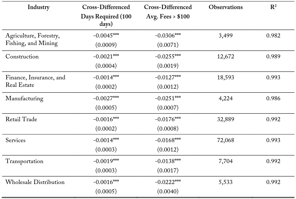
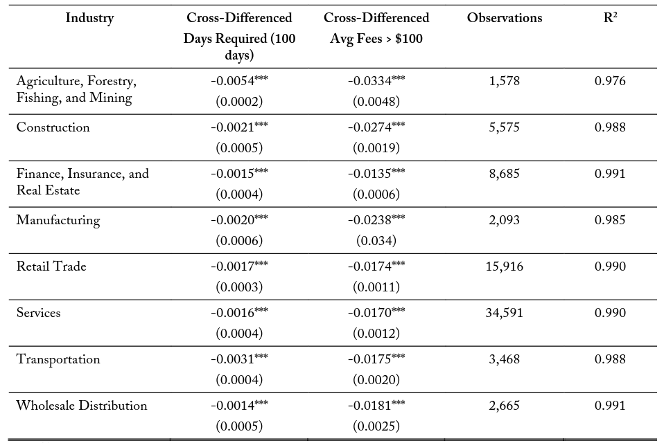
Table 8 explores potential differences in the correlation of occupational licensing costs and firm entry for various major industry classifications within a 10-kilometer buffer zone. These models are structured with the same control variable set at model (3) in tables 5-7. I find negative and significant marginal effects of an additional 100 days required on side 2 relative to side 1 for all industries. The correlations vary in magnitude from -0.0011 for the Services industry to -0.0032 for the Agricultural, Forestry, Fishing, and Mining industry. These industries with the larger coefficient estimate tend to be labor-intensive and are associated with better-known occupational license requirements. The average fees variable is also significant and negative across all specifications, ranging in magnitude from -0.0105 to -0.0267. Tables 9 and 10 repeat these industry specific models for the 5- and 2.5-kilometer border zones, respectively. These additional specifications maintain similar results in terms of magnitude, significance, and direction.
Since the data are cross-sectional, the results presented are meant only to be correlative and are not meant to make any causal claims. I find, using the DMT, that these firm location patterns around state borders are not arbitrary; instead, they are manipulated by entrants. Using a series of logistic regressions, I determine that there are significant negative marginal effects for both extra days required and a crossborder difference in monetary fees of greater than $100 in the firm entry decision for side 2. This means that when a state becomes more expensive relative to its adjacent state, firms are less likely to locate on the more expensive side of the border. These effects differ by industry and have larger magnitudes of marginal effects for firms in labor-intensive industries.
5.2 Firm Employment
In addition to firm entry decisions, I am also interested in the employment practices of firms. For example, it would make little empirical difference if we had twice the number of firms, provided those firms each had half as many employees. Therefore, both parts of the system must be analyzed. I use a geographic regression discontinuity design (GRDD) to determine if there is a systematic difference in average employment near state borders between high- and low-cost states. When considering areas within small buffer zones around state borders, this model assumes that that both sides of the border have similar populations of potential workers regarding density, education, and output quality. I also make the assumption that since these firms near state borders often make up a very small fraction of the total firms within a state, that they are not endogenously driving current occupational cost decisions at the state level. I believe these assumptions to be appropriate for considering the average number of workers per firm within small bins of distance on either side of the border, which abstracts away from the density of firms and employees.
Tables 12, 13, and 14 present the GRDD point estimates of the difference in employment trends at the border, when approaching over physical distance from the low-cost state on the left, and from the highcost state on the right. Table 12 shows the estimates at the 10-kilometer buffer zone. Column (1) is the basic GRDD point estimation for linear functions using a triangular kernel structure, bin width determined by minimizing the mean squared error, and standard errors clustered along the running 17 variable. The running variable in geographic regression discontinuity design framework is distance in the longitude and latitude space. Column (2) clusters the standard errors by the nearest neighbors along the running variable, by state. Column (3) allows for the non-linearity of the regressions on either side of the border by allowing polynomials of degree order 2. When analyzing changes in the average employee at 10 kilometers of distance, I find small and insignificant differences between the predicted border point estimates.
Table 13 limits the GRDD model to firms within a 5-kilometer buffer zone around the shared state borders. This specification may be more appropriate when analyzing border differences in average employment because occupational licensing cost effects may be larger for firms situated closer to an adjacent state. As with the 10-kilometer buffer, column (1) presents the base specification, column (2) clusters the standard errors by the nearest neighbor along the running variable by state, and column (3) allows for non-linearity of the regressions by allowing for higher order polynomials. In this specification I find that all models for the 5-kilometer border have significant, and negative, point estimation differences at the state border. The point estimation in the base model is -2.3421, indicating that there are approximately 2.3 fewer employees at a firm in the high-cost states relative to the low-cost states at the discontinuity. I likewise find a point estimation of -2.2896 in column (2) and -2.4453 in column (3). These results indicate that there are substantial firm average employment differences when considering firms within 5 kilometers of the state border.
The models are repeated for a 2.5-kilometer buffer zone in table 14. I find similar negative regression discontinuity point estimations, though not significant in column (3) when allowing for non-linearity of the regressions. Using this model and the limiting assumptions on the employee populations, there are potential concerns that these observations may be biased or influenced by other policies. To provide additional insight into the determinants of these employment differences, I conduct a comparative analysis on pairs of related industries that differ in occupational licensing requirements. These industry pairs are described in section 3.3. I conduct a series of non-temporal difference-in-difference (DD) models to compare licensed and unlicensed industries over state borders. The purpose of this analysis in conjunction with the GRDD is to determine if there are substantial differences in how licensed versus unlicensed firms differ in employment across high- and low-cost states.
Table 15 conducts the DD analysis for all firms found across the six matched industry pairs. The models for the six different match types are presented in tables 16–21. These results present three model specifications at the 20-, 10-, 5-, and 2.5-kilometer buffer zones. High Side and Licensed Industry represent indicator variables equal to 1 if the firm is located on the costlier side of the border pair and if it is part of a generally licensed industry, respectively. These coefficients do not provide much analytical insight, as they just account for differences within the industry and firm pair subsets. The variable of interest is the interaction term  , which is equal to 1 if the firm is both located on the costlier side of the border and is a licensed industry, and 0 otherwise.
The model specifications in Column (1) within table 15 represents the baseline specification where only the three variables of interest are regressed against the number of individuals a firm has employed. Within this specification, “high side” is determined by whichever side of the border has a longer amount of days required. Column (2) is the same specification, but the standard errors are clustered over bins of distance, as is common practice with geographic models in the longitude-latitude space. Column (3) also includes additional cross-differenced control variables.
I find that for the total firm model in table 15, the interaction term (H*OL) is consistently negative for all specifications and buffer zone distances. This coefficient represents a negative effect on firm employment for licensed firms in high-costs states that is not accounted for by differences in the border sides or differences between industries. Though the interaction term is not always significant, this may be due to an imprecise selection of controls. It is important to observe that the magnitude of this interaction effect in the total firms case is larger when considering firms in smaller buffer zones, in all specifications. For example, the most restrictive model presented in column (3) has a negative interaction coefficient of – 1.8648 when considering all firms within 20 kilometers of a state border. This means that licensed firms in high-cost states typically have 1.9 fewer employees, even when accounting for industry and border differences. When considering only firms within 10 kilometers of the state border, this interaction term increases in magnitude to -1.5785 and increases further to -3.9741 and -3.8537 for firms located within 5 and 2.5 kilometers of a state border, respectively.
The DD analysis is also conducted for the six match type pairs individually. These matches are pairs of industries that conduct similar functions within the economy but which differ in that one is often subject to occupational licensing for their workers while the other is not. Though these pairs of industries are similar, they are not perfect substitutes for one another. The analysis is meant to evaluate the validity of a possible interaction but not to make exhaustive causal claims. Table 16 compares the differences over borders for transportation industries, Match Type (1), with the licensed industry being Taxi Services (NAICS 485310) and the unlicensed industry being Other Transit and Ground Passenger Transit (NAICS 485999). When conducting the regression for this pair we find consistent yet insignificant interaction effects at 20, 5, and 2.5 kilometers. These effects become larger when analyzing subsets of firms closer to the border. These results, while they are not perfect specifications, support the possibility that there is an additional negative effect on employment for firms who are often subject to occupational licensing in high-cost states. In table 17, I find similar negative interaction terms for Match Type (2), architecture and design, which are also increasing in magnitude at smaller buffer sizes. Table 18, Match Type (3), comparing building repair industries, has a negative coefficient at 20 and 10 kilometers, which becomes positive at 5 kilometers and then negative again at the 2.5-kilometer buffer zone.
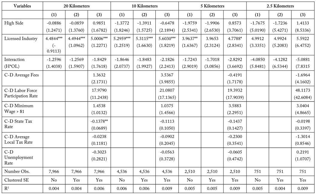
Table 19, Match Type (4), healthcare assistance, is the one subset group which does not exhibit these negative coefficients. Instead it finds a positive interaction term for typically licensed firms on the side of the border where employees lose more days of work to education and experience training. It is unknown if this feature is exclusive to the healthcare assistance industries, which may have greater benefits to 19 continuing education requirements for employees than other industries, possibly due to fast-paced advances in medical research. Tables 20 and 21—Match Type (5) comparing landscaping industries and Match Type (6) comparing lending industries—both exhibit a negative coefficient on employment for being a licensed industry firm in a costlier state relative to the adjacent state.
The DD models provide support that, though not perfectly specified or significant, there exists a potential negative effect on employment for licensed industries in states with a high cost of training days required relative to an adjacent state. This relationship persists, even when accounting for differences in the states and changes in employment for unlicensed industries. These DD models do require strong assumptions and are not significant in some instances—this is a limitation of this study and serves to identify important correlations rather than make causal claims. However, this correlative observation is reinforced by the GRDD point estimations of the average employee difference for the 10-, 5-, and 2.5-kilometer buffer zones. In summary, I find evidence of a negative impact on firm employment in high-cost states relative to adjacent low-cost states for firms near state borders.
6 Conclusion
In this study I analyze how occupational licensing costs impact firm entry and employment decisions near state borders. Although there has been significant research on product quality and consumer behavior in response to occupational licensing costs, no studies to my knowledge have attempted to determine how these costs affect firms in the latitudinal and longitudinal space over adjacent states. My improved webscraped data set of specific firm location information allows regression models to be conducted at finer levels of geography. With this sample, I am able to predict both changes to probability of firm entry location as well as changes in average firm employment.
I find that increasing the days required for education and experience training relative to an adjacent state or having average monetary fees greater than the adjacent state by over $100 correlates with a decrease in the probability of a firm entering the market on that side of the state border. These changes in probability are larger for labor-intensive and heavily regulated industries such as construction, manufacturing, wholesale distribution, agriculture, etc.
I find that when considering firms within a 5- or 2.5-kilometer buffer zone around a shared state boundary, there is a negative discontinuity point estimation between the low-cost and high-cost states in average firm employment. This means that there is a significant difference in the expected average number of employees at the state border between low- and high-cost state pairs, and that high-cost states have fewer expected employees than low-cost states. To substantiate the validity of these observations, I compare the average firm employment of pairs of similar licensed and unlicensed industries over state borders. I observe a negative effect in the interaction of being a licensed industry and residing in a highcost state on the number of employees a firm has on its payroll.
These findings have several implications for policymakers. With a growing percentage of the US workforce requiring an occupational license, understanding the implications of these policies on firm outcomes is crucial for fostering business and economic growth. My results suggest that states can attract new businesses and improve overall employment through small changes in cost requirements for occupational licenses relative to adjacent states, which can have a variety of public policy effects. While my findings have limitations due to the cross-sectional nature of the data, this study serves as an exploratory introduction into to the influence of occupational licensing costs on firms.
Appendix A: Border Zone Design
There are 109 different state border pairs, including a few that consist of a single point, such as GeorgiaNorth Carolina. For the empirical results, I conduct this analysis on buffer zone sizes of 1, 5, and 10 kilometers. First, I use geographic information systems (GIS) to overlay my cross-sectional firm location data from April 2017 onto detailed state maps. I use the longitude and latitude for the location of each firm to determine both the firm’s exact location on a map and its distance from other geographic features. I identify the shortest possible distance from each firm to its closest state border containing two or more states. I then use GIS to draw buffer zones around state borders and identify each firm that falls within particular ranges of distance. For graphical illustration, figure 2 shows a map of the 299,746 businesses launched within a 10-kilometer buffer of a state border pair. Figure 3 provides a zoomed-in look at a selection of states.
Figure 2. Map of Firm Locations within 10 km of a State Border Pair
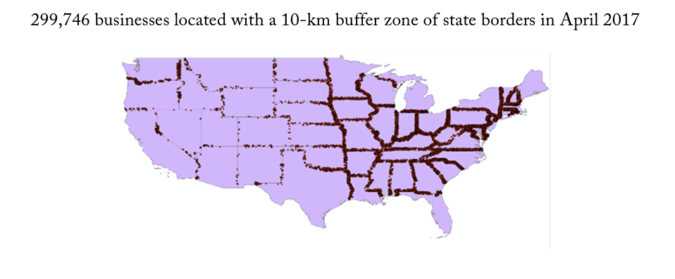
Figure 3. Zoomed-in Map of Firm Locations within 10 km of a Border Pair
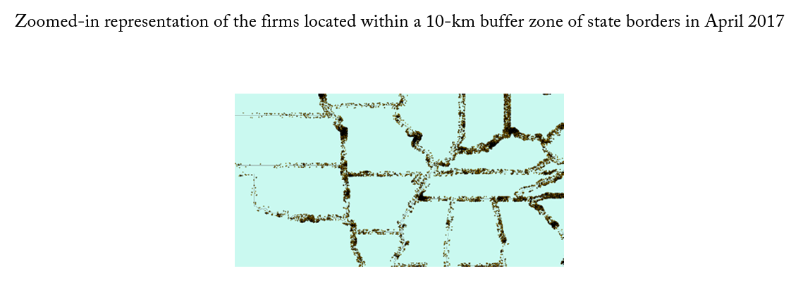
Table 1. Summary Statistics
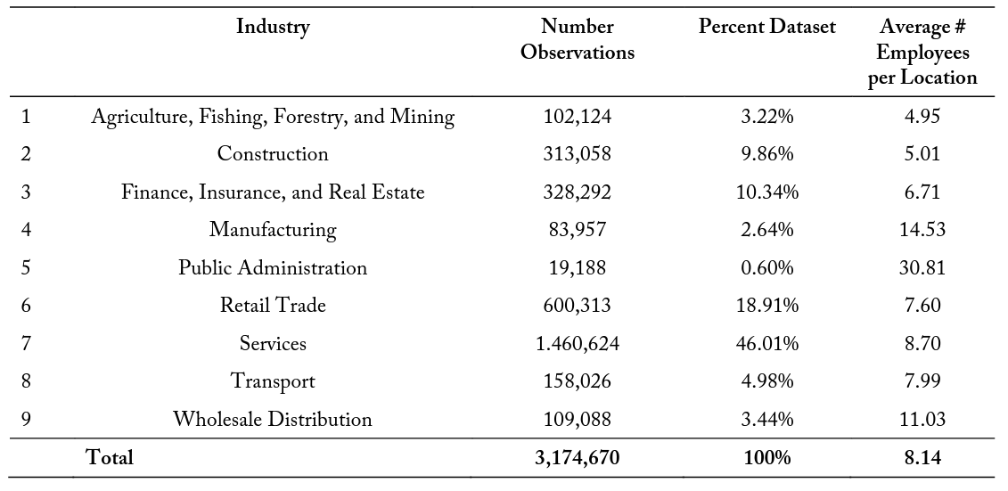
Table 2. Match Industry Pairs
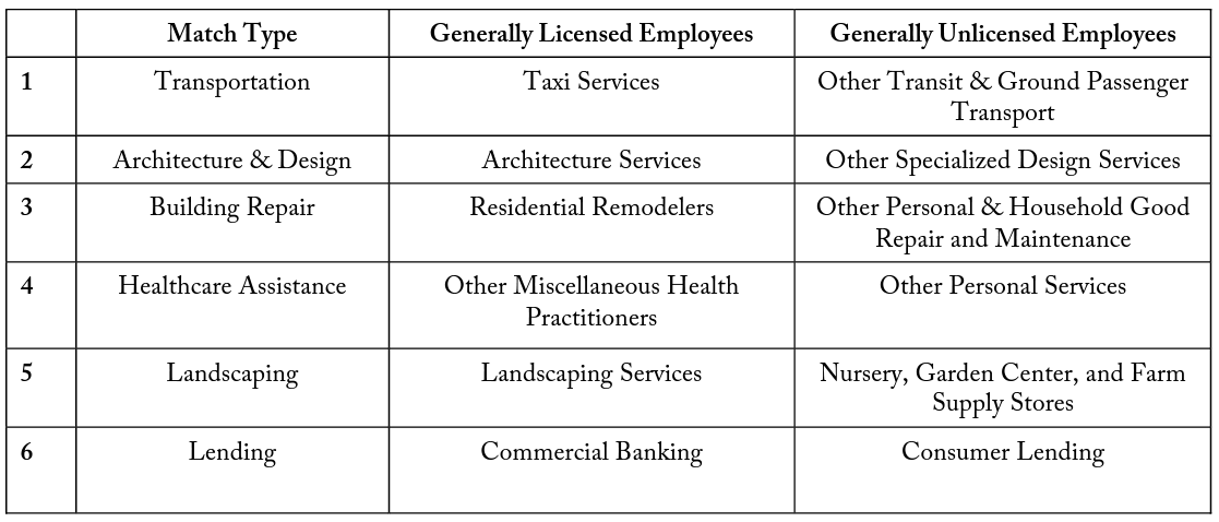
Figure 4. Density of Firms around Border
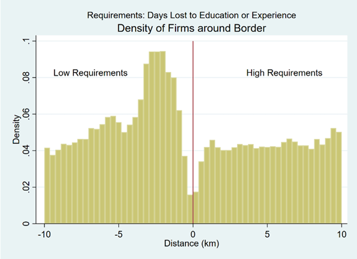
Table 3. Summary Statistics of State Variables
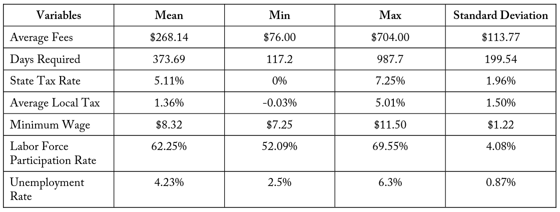
Table 4. Summary Statistics of Cross-Differenced State Variables
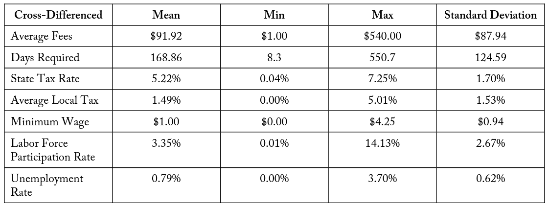
Table 5. Logit Function for Days Required within 10 km
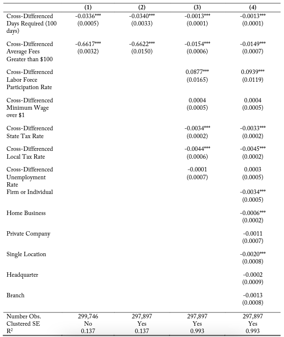
Notes: Each coefficient represents the change in the probability of electing onto a side of the border based upon a change in the variable. For example, in column (1), a 100-day increase in the days of education and experience requirement relative to the other side decreases the probability of electing onto that side of the border by 3.36 percent. A state being more expensive than the adjacent state by more than $100 reduces the probability by 66.17 percent.
Table 6. Logit Function for Days Required within 5 km
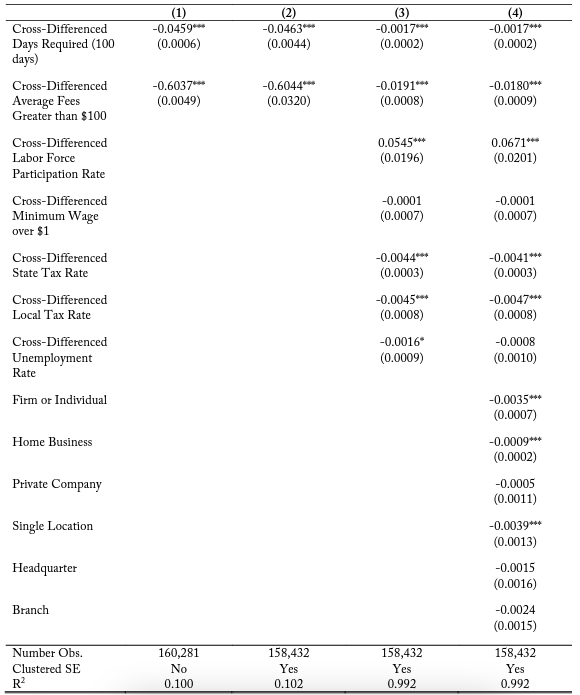
Notes: Each coefficient represents the change in the probability of electing onto a side of the border based upon a change in the variable. For example, in column (1), a 100-day increase in the days of education and experience requirement relative to the other side decreases the probability of electing onto that side of the border by 4.59 percent. A state being more expensive than the adjacent state by more than $100 reduces the probability by 60.37 percent.
Table 7. Logit Function for Days Required within 2.5 km
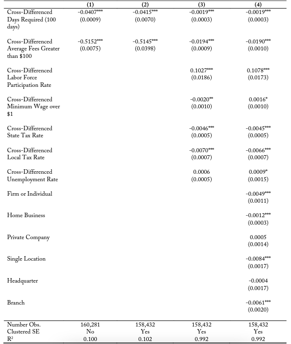
Notes: Each coefficient represents the change in the probability of electing onto a side of the border based upon a change in the variable. For example, in column (1), a 100-day increase in the days of education and experience requirement relative to the other side decreases the probability of electing onto that side of the border by 3.36 percent. A state being more expensive than the adjacent state by more than $100 reduces the probability by 66.17 percent.
Table 8. Logit Function on Days Required within 10 km of Border, by Industry
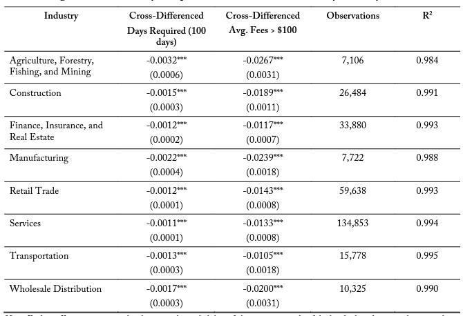
Notes: Each coefficient represents the change in the probability of electing onto a side of the border based upon a change in the variable, separated by industry. Though not depicted, each of these regressions includes cross-border state controls. For example, for Construction, a 100-day increase in the days of education and experience requirement relative to the other side decreases the probability of electing onto that side of the border by 0.15 percent. A state being more expensive than the adjacent state by more than $100 reduces the probability by 1.89 percent.
Table 9. Logit Function on Days Required within 5 km of Border, by Industry
 Notes: Each coefficient represents the change in the probability of electing onto a side of the border based upon a change in the variable, separated by industry. Though not depicted, each of these regressions includes cross-border state controls. For example, for Construction, a 100-day increase in the days of education and experience requirement relative to the other side decreases the probability of electing onto that side of the border by 0.21 percent. A state being more expensive than the adjacent state by more than $100 reduces the probability by 2.55 percent.
Table 10. Logit Function on Days Required within 2.5 km of Border, by Industry
 Notes: Each coefficient represents the change in the probability of electing onto a side of the border based upon a change in the variable, separated by industry. Though not depicted, each of these regressions includes cross-border state controls. For example, for Construction, a 100-day increase in the days of education and experience requirement relative to the other side decreases the probability of electing onto that side of the border by 0.21 percent. A state being more expensive than the adjacent state by more than $100 reduces the probability by 2.74 percent.
Table 11. Density Manipulation Test
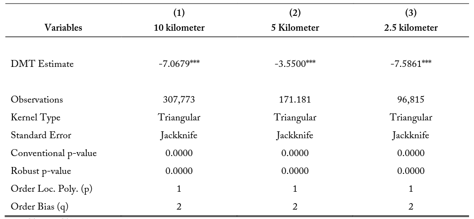
Notes: The DMT Estimate represents the difference in the density of firms on either side of the state border and identifies if these location decisions could have been due to random chance.
Table 12. GRDD: Employment within 10 km of Border
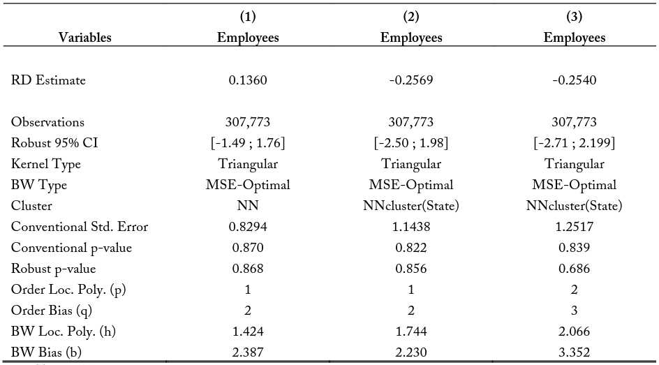
Notes: The RD Estimates represent the difference in the point estimate at the border when approaching the state border from either state interior. For example, the estimate for model (3) shows when considering all the first within a 10-kilometer buffer of the state border, the model predicts firms from the state with the higher education and experience requirements will have 0.2540 fewer employees on average.
Table 13. GRDD: Employment within 5 km of Border

Notes: The RD Estimates represent the difference in the point estimate at the border when approaching the state border from either state interior. For example, the estimate for model (3) shows when considering all the first within a 5-kilometer buffer of the state border, the model predicts firms from the state with the higher education and experience requirements will have 2.4453 fewer employees on average.
Table 14. GRDD: Employment within 2.5 km of Border
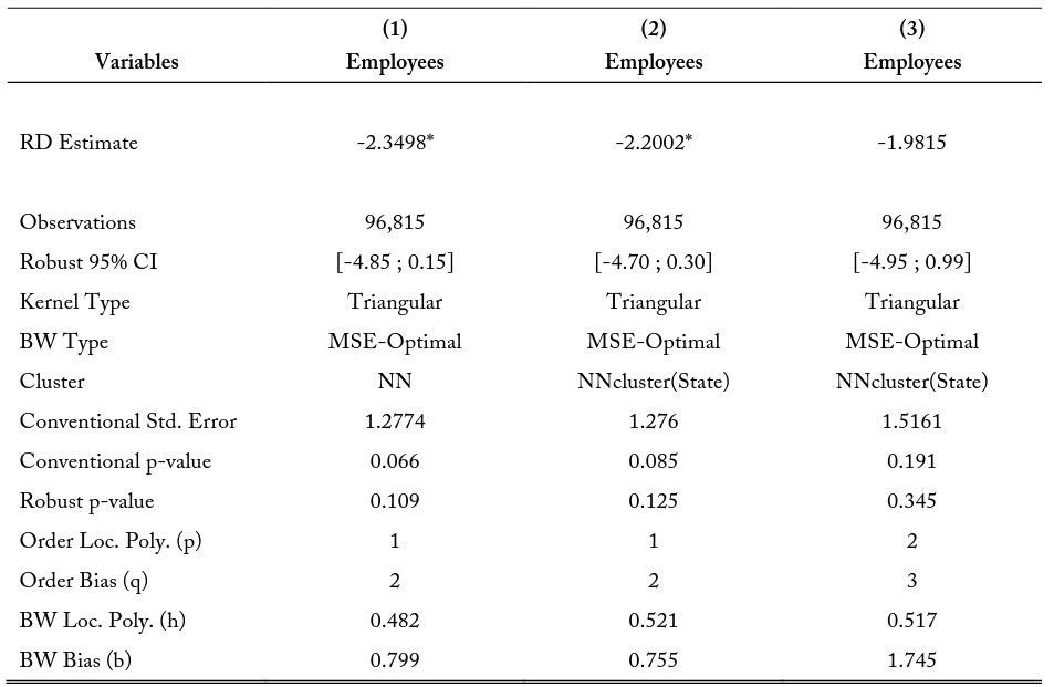
Notes: The RD Estimates represent the difference in the point estimate at the border when approaching the state border from either state interior. For example, the estimate for model (3) shows when considering all the first within a 2.5-kilometer buffer of the state border, the model predicts firms from the state with the higher education and experience requirements will have 1.9815 fewer employees on average.
Table 15. Difference-in-Difference for Firm-Industry Pairs: All Groups
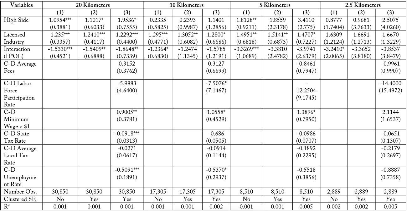
Table 16. Difference-in-Difference for Firm-Industry Pairs: Group Pair 1
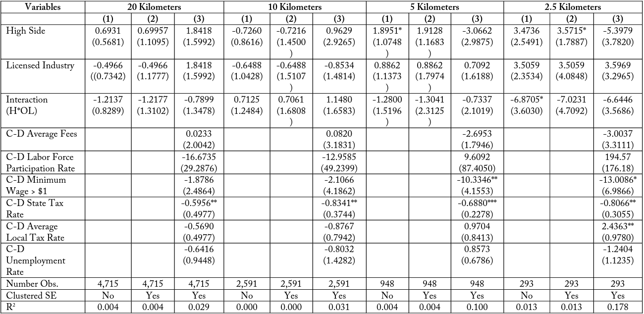
Table 17. Difference-in-Difference for Firm-Industry Pairs: Group Pair 2
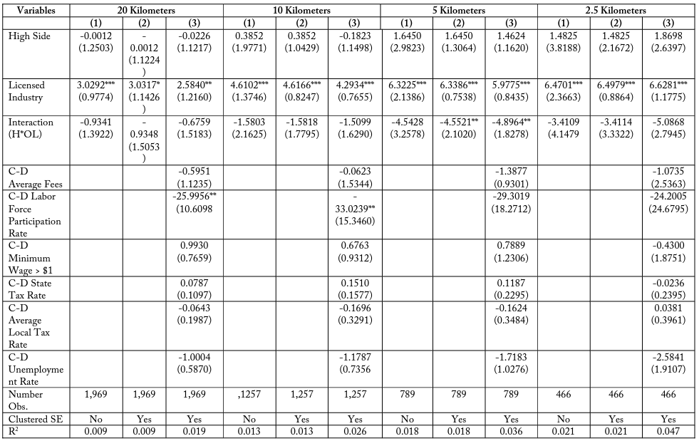
Table 18. Difference-in-Difference for Firm-Industry Pairs: Group Pair 3
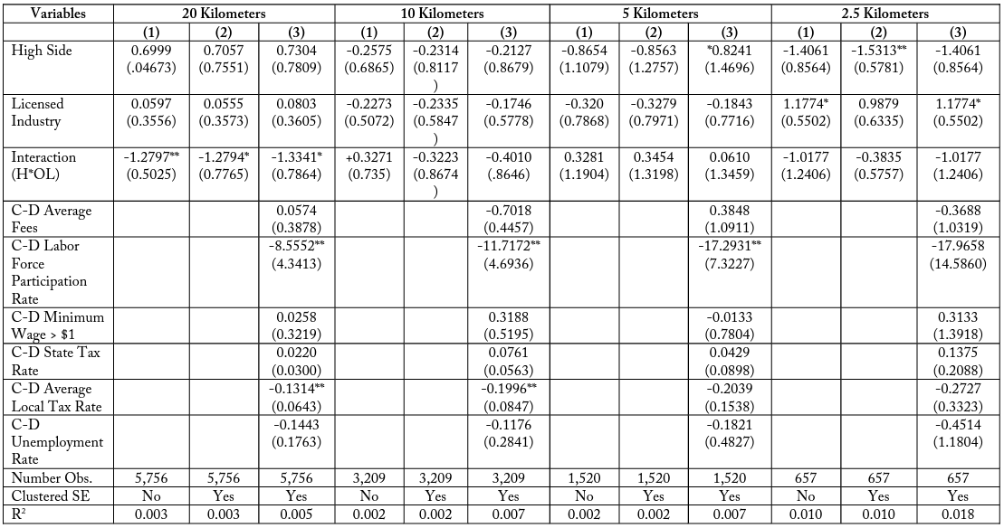
Table 19. Difference-in-Difference for Firm-Industry Pairs: Group Pair 4
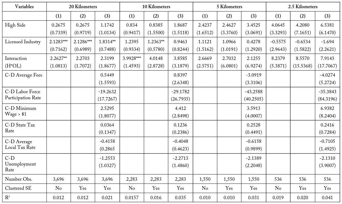
Table 20. Difference-in-Difference for Firm-Industry Pairs: Group Pair 5
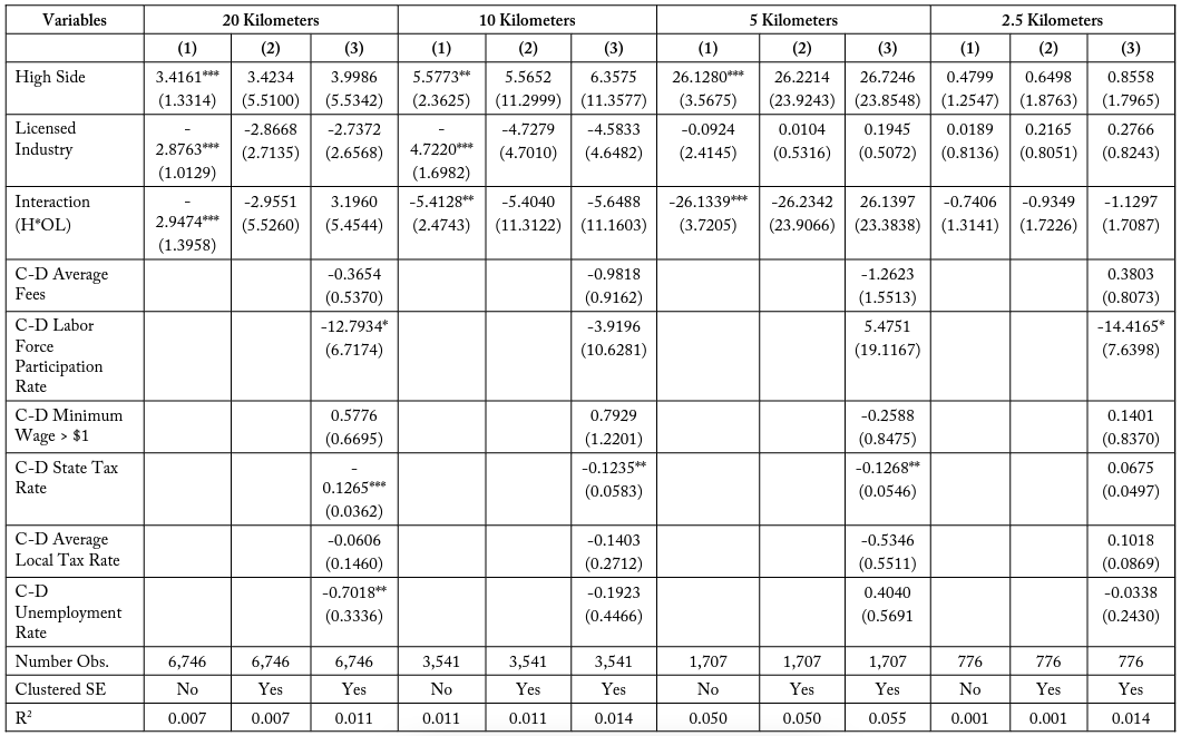
Table 21. Difference-in-Difference for Firm-Industry Pairs: Group Pair 6
References
Adams, F. A., Jackson, J. D., & Ekelund, R. B. (2002). Occupational licensing in a ‘competitive’ labor market: The case for cosmetology. Journal of Labor Research, 23(2), 261–278.
Akerlof, G. (1970). The market for lemons: Qualitative uncertainty and the market mechanism. Quarterly Journal of Economics, 84(August), 488–500.
Angrist, J. D., & Guryan, J. (2008). Does teacher testing raise teacher quality? Evidence from state certification requirements. Economics of Education Review, 27(5), 483–503.
Arrow, K. (1971). Essays in the theory of risk-bearing. Markham Publishing.
Blair, P. Q., & Chung, B. W. (2018). How much of a barrier to entry is occupational licensing? (Working paper No. 25262). National Bureau of Economic Research. doi:10.3386/w25262
Bond, R. S., Kwoka, J. E., Jr., & Whitten, I. T. (1980). Staff report on effects of restrictions on advertising and commercial practice in the professions: The case of optometry (United States, Federal Trade Commission, Bureau of Economics).
Card, D., & Krueger, A. B. (1994). Minimum wages and employment: A case study of the fast-food industry in New Jersey and Pennsylvania. The American Economics Review, 84(4), 772–793.
Carroll, S. L., & Gaston, R. J. (1981). Occupational restrictions and the quality of service received: Some evidence. Southern Economic Journal, 47(4), 959–976.
Cattaneo, M. D., & Escanciano, J. C. (2017). Regression Discontinuity Designs: Theory and Applications. Emerald Insight.
Cattaneo, M. D., Idrobo, N., & Titiunik, R. (in press). A practical introduction to regression discontinuity designs (Vol. 1). Cambridge University Press.
Cattaneo, M. D., Jansson, M., & Ma, X. (2018). Manipulation testing based on density discontinuity. Stata Journal, 18(1), 234–261.
Cheng, M. (1997). Boundary aware estimators of integrated density products. Journal of the Royal Statistical Society, 59(1), 191–203.
Conrad, D. A., & Sheldon, G. G. (1982). The effects of legal constraints on dental care prices. Inquiry, 19(1), 51–67.
Cox, C., & Foster, S. (1990). The costs and benefits of occupational regulation (United States, Federal Trade Commission, Bureau of Economics). U.S. Government Printing Office.
Dell, M. (2010). The persistent effects of Peru’s mining Mota. Econometrica, 78(6), 1863–1903.
Federman, M. N., Harrington, D. E., & Krynski, K. J. (2006). The impact of state licensing regulations on low-skilled immigrants: The case of Vietnamese manicurists. The American Economic Review, 96(2), 237–241.
Gittleman, M., Klee, M. A., & Kleiner, M. M. (2017). Analyzing the labor market outcomes of occupational licensing. Industrial Relations, 57(1), 57–100.
Guis, M. (2016). The effects of occupational licensing on wages: A state level analysis. International Journal of Applied Statistics, 13(2), 30–45.
Haas-Wilson, D. (1986). The effect of commercial practice restrictions: The case of optometry. The Journal of Law and Economics, 29(1), 165–186.
Holen, A. S. (1965). Effects of professional licensing arrangements on interstate labor mobility and resource allocation. Journal of Political Economy, 73(5), 492–498.
Johnson, J. E., & Kleiner, M. M. (n.d.). Is occupational licensing a barrier to interstate migration? (United States, Federal Reserve Bank of Minneapolis, Research Division). Staff Report 561.
Kane, T. J., Rockoff, J. E., & Staiger, D. (2008). What does certification tell us about teacher effectiveness? Evidence from New York City. Economics of Education Review, 27(6), 615–631.
Keele, L., Titiunik, R., & Zubizarreta, J. R. (2015). Enhancing a geographic regression discontinuity design through matching to estimate the effect of ballot initiatives on voter turnout. Journal of the Royal Statistical Society, 178(1), 223–239.
Kleiner, M. M. (2017, July). Regulating access to work in the gig labor market: The case of Uber. W. E. Upjohn Institute for Employment Research Employment Research Newsletter, 24 (3), 4–6.
Kleiner, M. M., & Krueger, A. B. (2010). The prevalence and effects of occupational licensing. British Journal of Industrial Relations, 48(4), 1–12.
Kleiner, M. M., & Krueger, A. B. (2013). Analyzing the extent and influence of occupational licensing on the labor market. Journal of Labor Economics, 31(2), S173–S202.
Kleiner, M. M., & Kudrle, R. R. (2000). Does regulation affect economic outcomes? The case of dentistry. The Journal of Law and Economics, 43(2), 547–582.
Kleiner, M. M., & Park, K. W. (2010). Battles among licensed occupations: Analyzing government regulations on labor market outcomes for dentists and hygenists (pp. 1–40, Working paper No. 16560). NBER.
Kleiner, M. M., & Vorotnikov, E. (2017). Analyzing occupational licensing among the states. Journal of Regulatory Economics, 52(2), 132–158.
Law, M. T., & Kim, S. (2005). Specialization and regulation: The rise of professionals and the emergence of occupational licensing regulation. The Journal of Economic History, 65(3), 723–756.
Maurizi, A. R. (1980). The Impact of Regulation on Quality: The Case of California Contractors. In Occupational Licensure and Regulation (pp. 26-47). Washington D.C.: American Enterprise Institute Press.
McCrary, J. (2008). Manipulation of the running variable in the regression discontinuity design: A density test. Journal of Econometrics, 147, 698–714.
Meehan, B., Timmons, E., & Meehan, A. (2017). Barriers to mobility: Understanding the relationship between growth in occupational licensing and economic mobility (Rep.). Archbridge Institute.
Pashigian, B. P. (1979). Occupational licensing and the interstate mobility of professionals. The Journal of Law and Economics, 22(1), 1–25.
Perloff, J. M. (1980). The impact of licensing laws on wage changes in the construction industry. The Journal of Law and Economics, 23(2), 409–428.
Shapiro, C. (1986). Investments, moral hazard, and occupational licensing. The Review of Economic Studies, 53(5), 843–862.
Slivinski, S. (2017). Weighing down the bootstraps: The heavy burden of occupational licensing on immigrant entrepreneurs (pp. 1–12, Rep. No. 2017-01). Center for the Study of Economic Liberty at Arizona State University.
Timmons, E., & Thorton, R. (2008). The effects of licensing on the wages of radiologic technologists. Journal of Labor Research, 29(4), 333–346.
U.S. Bureau of Labor Statistics. (2016). Data on certificates and licensing. http://www.bls.gov/cps/certifications-and-licenses.htm#highlights.
Van Stel, A., Storey, D. J., & Thurik, A. R. (2007). The effect of business regulations on nascent and young business entrepreneurship. Small Business Economics, 28(2/3), 171–186.
Zapletal, M. (2018). The effects of occupational licensing: Evidence from business-level data. British Journal of Industrial Relations, 1–25.