The US Postal Savings System and the Collapse of Building and Loan Associations during the Great Depression

Introduction

Regulatory competition is often blamed for causing financial crises. For example, studies have highlighted the instigating role of trust companies in the Panic of 1907 (Moen and Tallman 1992), saving and loans associations (S&Ls) in the S&L crisis (Shoven et al. 1992), and shadow banks in the Great Recession (Gertler and Gilchrist 2018). Typically, this outcome occurs due to the attraction of funds to less regulated and more risky financial institutions that offer a high return. However, regulatory competition also worsens financial crises when they do occur as investors often shift funds into commodities such as gold, which extends runs on institutions, and as commercial banks accumulate reserves at the Fed, which prevents funds from being put to use in the community. This paper examines whether this dynamic could partially be responsible for the slow rebound of the mortgage market during the Great Depression. O’Hara and Easley (1979) blame the federally insured US Postal Savings System for attracting needed funds from building and loan associations (B&Ls) during the 1930s, which prevented them from supporting the mortgage market. O’Hara and Easley show a negative correlation between B&Ls and postal savings at the national level, but lacking disaggregated data, they are not able to rule out alternative explanations and reverse causality. In this paper, we use annual town-level data from 1920 to 1935 on both B&Ls and postal savings depositories to formally test this relationship by comparing changes in deposits in institutions in the same location during the same year.

The US Postal Savings System (1911–67) was created to offer the unbanked and marginalized households a fully guaranteed deposit account at post offices. While the system was disbanded in 1966, its reestablishment has become an increasingly prominent modern prescription to address the gap in affordable banking options for low-income households. For example, Sen. Bernie Sanders has proposed its reestablishment in his 2016 and 2020 presidential campaigns, and Sen. Kirsten Gillibrand proposed legislation in 2018 to not only re-establish the system but also allow check cashing and loan services. Despite the renewed interest, however, we know little about how the postal savings system affected other financial institutions.

The literature on postal savings banks has focused on the patterns of usage (Kemmerer 1917; Schewe 1971; Sprick Schuster et al. 2019) or on postal savings’ response to commercial bank failures (Sissman 1936; Kuwayama 2000; Davidson and Ramirez 2016). Meanwhile, the literature on B&Ls has focused on their popularity at an aggregate level (e.g., Clark and Chase 1925; Bodfish 1931, 1935) or the role they played in the success of the mortgage market during the 1920s and 1930s (Courtemanche and Snowden 2011; Fishback et al. 2011, 2013, and 2019; Rose 2014; Fleitas et al. 2018). O’Hara and Easley (1979)is the one study that examines the competition between postal savings banks and B&Ls. The authors argue that postal savings drew funds from B&Ls. Unlike commercial banks, B&Ls were prohibited from receiving redeposits from postal savings banks and sought out the same small private savers that postal savings banks did. Lacking disaggregated data that have only recently become accessible to researchers, O’Hara and Easley are not able to test for a causal relationship between B&Ls and postal savings usage. For instance, the government guarantee of postal savings deposits would have attracted funds during the Great Depression regardless of the presence of B&Ls, and B&Ls would likely have struggled during the real estate price decline regardless of the presence of a postal savings bank.

To provide a comprehensive analysis of the competition between postal savings banks and B&Ls, we com- bine annual town-level data for three representative states from 1920 through 1935, allowing us to address potential reverse causality while controlling for unobserved heterogeneity across towns and across time. In this way, we can be sure that the results are not being spuriously driven by the nature of the Great Depres- sion or differential selection of financial institutions across towns. Instead, we identify the relationships using deposit changes in B&Ls and postal savings depositories in the same location in the same year.

The results of a panel vector autoregression (Panel VAR) show that level of postal savings deposits have a negative and statistically significant effect on the total value of B&L shares, but B&L share value does not have a statistically significant effect on postal deposits. Impulse response functions (IRFs) show that a positive shock to postal savings deposits leads to a persistent decline in B&L share value. These results hold even after controlling for town population growth and commercial bank activity. We thus confirm that the existence of a federally insured deposit alternative for small depositors drew funds from B&Ls during the Great Depression and may even have prevented a quick return to normal conditions after the banking panics subsided.

Background on Postal Savings Banks and B&Ls

The US Postal Savings System offered individuals the ability to start savings accounts at thousands of local post offices.¹See Sprick Schuster et al. (2019) for a discussion of the political economy of the Postal Savings System. Postal deposits earned a fixed rate of 2 percent nominal simple interest and was fully insured by the US government. In order to prevent competition with commercial banks, postal savings redeposited nearly all of its funds in commercial banks and did not make any loans. The system thus offered a guaranteed return for all depositors throughout the period, and its services did not vary during the Great Depression.

B&Ls were local, cooperative institutions that specialized in residential mortgage lending. What set B&Ls apart from commercial banks was their share accumulation contracts (SACs). The SACs allowed borrowers to repay mortgage debt gradually by buying shares of the associations, rather than making a single final payment as with the balloon contracts at commercial banks.²The SAC is a combination of, first, an interest-only balloon loan with an indefinite maturity for which the borrower made monthly interest payments and, second, a pledge to purchase installment equity shares in the association until they were equal in nominal value to the principal of the loan. The shares paid interest based on the B&Ls’ loan portfolio and thus could lengthen or shorten the loan contract. The shares generally achieved a high return for their investors, but that return varied across local real estate markets.

B&Ls attracted both borrowing and nonborrowing members. As nonborrowing members, like borrowing members, had to purchase shares of the associations (instead of holding regular deposits), both types of members were owners of the association with “one member, one vote” voting rights, had equal shares in profits and losses, and had very limited withdrawal privileges. A nonborrower “withdrawal” involved the repurchase of their equity by the remaining owners in the association. Withdrawals thus decreased the liquidity of the association, and B&Ls had penalties for those made before the date of full maturity (Clark and Chase 1927).³Withdrawal policies had become more liberal in the 1920s with the rapid expansion of investments in B&Ls, even suspending withdrawal penalties. However, the liberalization was undone in the 1930s because of the reduced inflow of new members, defaults on outstanding loans, and state laws that explicitly restricted withdrawals (Snowden 2003). While informal secondary markets appeared in some larger cities to provide liquidity, B&L shares were purchased at very discounted prices relative to their book value (Rose 2014; Kendall 1962).

B&Ls dramatically changed in the mid-1930s as a result of new policies established to improve the mortgage market and to help B&Ls replace their SACs with direct reduction contracts⁴Under DRCs, borrowers paid monthly interest and principal payments to their bank. (DRC) and convert themselves into S&Ls.⁵The Federal Housing Administration mortgage-loan insurance program, which amortized DRC loans that ran for fifteen years or more, was one of these programs (Snowden 2010). As a result, S&Ls became the dominant mortgage lenders by the beginning of the 1940s, and B&Ls dramatically declined in number and importance (Rose 2014; Rose and Snowden 2013; Snowden 2003 and 2010). The government assisted B&Ls during the mid-1930s through direct lending, purchases of distressed mortgages, and the liberal refinancing of loans, thus changing the behavior of the remaining B&Ls going forward.⁶ For instance, the Federal Home Loan Bank (FHLB) system and the Reconstruction Finance Corporation provided short-term loans to B&Ls (Vossmeyer 2016) while the Home Owners’ Loan Corporation purchased distressed mortgages and refinanced loans on more liberal terms. Note that the state of New York organized its own “FHBL” in 1916 (Frame, Hancock and Passmore 2012). By 1927, about half of New York’s B&Ls had joined this institution, and by 1940, about half of those firms had also joined the federal FHLB while staying in the state FHLB.

Usage trends differed greatly between postal savings and B&Ls. Figure 1 compares postal savings banks’ and B&Ls’ usage patterns between 1920 and 1940 for our three sample states (New York, South Carolina, and Wisconsin). Postal savings were decreasing in popularity during the 1920s, but the Great Depression led to a sudden expansion. Between 1930 and 1934, the amount on deposit at post offices increased by more than 400 percent. In contrast, B&Ls expanded rapidly in the 1920s, financing 4.2 million of the 7 million homes built during that decade. Then, between 1930 and 1934, total B&L share value fell by over 25 percent and only rebounded slightly going forward.

The negative correlation in figure 1 between postal savings deposits and B&L share value suggests competition between postal savings banks and B&Ls, but there are additional reasons to believe the two competed with each other. Sprick Schuster et al. (2019) argue that the surge of postal savings deposits in the 1930s was the result of a flight to quality. Representative Emanuel Celler of New York stated that “while banks were failing all over the country and a veritable avalanche of funds came out of other banks, it was the Postal Savings System that salvaged much of the money withdrawn by the frightened and the timid” (Congressional Record, December 9, 1931, p. 235). Both postal savings and B&Ls appealed to small- scale and probably relatively risk-averse customers.⁷The requirement that postal savings be redeposited in commercial banks was an explicit attempt to eliminate any competition between the two types of institutions. The approach was the result of the very effective commercial bankers’ lobby association, the American Bankers Association. The lack of any concessions for B&Ls is likely due to their relatively small numbers when the Postal Savings Act was passed in 1911. A congressional representative even highlighted this specific competition: “There is practically no money in the state available for home financing. The money which ordinarily would find its way into S&Ls is either hoarded in safety deposit boxes or deposited in postal savings” (cited in O’Hara and Easley 1979, p. 748). Moreover, while B&Ls were previously able to attract and retain investors because of their high dividend payments compared to the low but fixed interest on postal savings, this advantage disappeared during the 1930s as foreclosures and the lack of new loans led to much lower returns on mortgages.

The competition took place on at least two dimensions. First, investors could have been tempted to withdraw their investments in B&Ls and deposit them in postal saving banks. However, while B&Ls often allowed withdrawals by nonborrower members in the 1920s, the directors largely suspended withdrawals during the 1930s and borrowing members opposed the liquidation of insolvent associations until their loans had been paid off (Fleitas et al. 2018). Therefore, while nonborrower investors might have wanted to withdraw their money for better opportunities, many could not quickly liquidate their shares. Second, postal savings banks may have competed away new business that would have otherwise gone to B&Ls.

New investors during the Depression may have avoided the low returns and potential lock-in of B&L shares and turned to the guaranteed fixed return and liquidity of postal savings. The rest of the paper uses new town-level data on both B&L shares and postal savings deposits to tease out the relationship between the two institutions.

Data and Empirical Analysis

Postal savings data come from Sprick Shuster et al. (2019). The papers’ authors digitized the annual amount of deposits in each post office from the Annual Reports on the Operation of the Postal Savings System. The data on B&Ls come from Fishback et al. (2019). The paper’s authors digitized the name, location, and annual balance sheet of each B&L from the state banking and insurance reports of New York, North Carolina, and Wisconsin between 1920 and 1935.⁸ See appendix table A.1 for summary statistics on each state. While Fishback et al. (2019) have data for Iowa and Fleitas et al. (2018) have data for New Jersey, we do not include those data here because information is missing for the 1920s. B&L data were aggregated up to the town/village/ hamlet level to match the postal-deposit data. We measure depositor activity in B&Ls by the value of all outstanding shares⁹There is heterogeneity across the three states in the way they present the information on B&L balance sheets. Fishback et al. (2019) create categories of balance sheet variables that are standardized across states. We use the “shares” category, which includes installment shares and other balance sheet categories that reflect deposits, such as paid-up shares, income shares, and one-payment shares. and depositor activity in postal savings banks by total deposits. Our sample stops in 1935 in order to avoid the confounding effects of the conversion of B&Ls into S&Ls and governmental policies implemented to directly assist B&Ls in the second half of the thirties.

While postal deposits could be made in virtually any post office, B&Ls were not present in many cities. Since we are focused on the competition between B&Ls and postal savings deposits rather than the total growth of postal savings (previously studied by Sprick Shuster et al. 2019), we constrain our analysis to any town/year combination in which a B&L is observed. Clearly, there can be no competition between B&Ls and postal savings in places where B&Ls do not exist.¹⁰The inverse is not true. In places with B&Ls and no observed postal savings activity, B&Ls could have affected postal savings anyway, especially since each place had a post office. The Post Office constantly re-evaluated the placement of postal depositories, and post offices lost and gained depositories frequently. In fact, it is at times difficult to determine whether a town lacked a postal depository or whether there happened to be $0 on deposit. At an aggregate level, B&Ls had steeper declines during the Great Depression in places with positive values of postal savings, and postal savings had higher growth in locations with B&Ls. When adding the places that never had a B&L to our regressions, we obtain similar point estimates, although the effect is more imprecisely estimated. The map in figure 2 shows that the 387 towns with a B&L and a listed post office (i.e., those included in our sample) are not biased toward a particular geographic area nor significantly different from those cities that had a listed post office but never had a B&L. If anything, B&Ls are clustered in larger cities with sufficient housing demand whereas postal savings offices were located throughout each of the states.

This sample is representative of the nation during the twenties and the first half of the thirties. The three states we examine represent different parts of the country and have large and diverse economies as measured by share of employment in various industries: New York has financial markets and manufacturing, North Carolina has cotton and tobacco agriculture, and Wisconsin has corn, wheat, and dairy agriculture. Moreover, the B&L industry in all of these states expanded during the twenties and contracted during the Depression, matching the national-level B&L trends.

The goal of this paper is to disentangle the relationship between B&Ls and postal savings. Because we do not want to impose a particular pre-existing relationship, we proceed with a panel VAR approach.¹¹We make use of the code provided in Love and Zicchino (2006). As a robustness check, we also calculate impulse responses using the local projection method ( Jordà 2005). This approach provides similar results for the effect of postal deposits but shows a greater role for B&L share values. Given the relatively small number of time observations per city, we prefer the panel VAR method to linear projection (Kilian and Kim 2011). The VAR methodology allows the variables of interest to enter into a system of equations as endogenous, enabling us to estimate the bidirectional relationship between postal savings deposits and B&L usage. The panel-data approach allows us to control for unobserved heterogeneity across towns and across time. The identifying variation comes from changes over time at the town level, controlling for time-invariant town effects and general time trends. We thus can be sure that our estimated coefficients are not being driven by differential selection of B&Ls and postal depositories into particular areas of the country or the general effect of the Great Depression itself. We also include the population of each location as an exogenous control for the growth in the supply of investment funds in any particular area.¹²Population comes from the Census of Population each decade. Values in between observations are filled with a linear trend.

Indeed, a threat to identification in our setting is unobserved town-level factors correlated over time with the differential behavior of deposits in both postal savings and B&Ls that is not correlated with population growth. For example, for our results to overestimate the negative effect of postal savings banks on B&Ls, there would have to be some time-varying unobserved factors at the town level that are responsible for both the decline of postal savings and rise of B&Ls during the 1920s and the rise of postal savings and decline of B&Ls during the 1930s. While we do not have town-level data on factors that could be declining during the Great Depression such as income and employment, the results are not sensitive to aggregating to the county level or to including annual total tax returns instead of the interpolated town population.¹³We prefer using population because it does not require aggregating to the county level and studying competition between institutions that could be many miles apart. So it is unlikely that any particular unobserved variable could be driving the result.

To estimate competition between B&Ls and postal savings banks from 1920 to 1935, we use the follow- ing system of equations:

(1)  

is a vector of endogenous variables (natural log of postal deposits; natural log of B&L shares), is a set of lags for each of the dependent variables, is the natural log of population of each location, is a vector of year fixed effects that capture common, year-specific shocks, is a vector of town-specific fixed effects, and is a robust error term.¹⁴We convert all variables into log form (after adding 1). We select one lag based on the modified Akaike information criterion, the modified Bayesian information criterion, and the modified Hannan-Quinn information criterion. We also confirm that the system satisfies the necessary stability conditions using the unit root test (see appendix figure A.1). Fixed effects are removed using forward orthogonal deviation (the Helmert procedure).

In choosing the Cholesky ordering of the endogenous variables, we assign the total value of B&L shares a higher order and assume postal deposits can only affect B&L share value with a lag for two reasons. First, we believe that B&L share value is more exogenous than postal deposits. For instance, an increase in foreclosures could reduce the value of B&L shares without having any direct effect on postal deposits. Second, B&L shares faced restrictions on withdrawal. Therefore, even if a depositor wanted to cash in their B&L shares and make a deposit in a postal savings account, they could not always do so, particularly during the 1930s. Note also that the ordering chosen introduces a bias away from finding an effect of postal savings deposits on B&L share value and toward an effect of B&L share value on postal savings deposits. Indeed, when we reverse the ordering of the two institutions, the effect of postal savings deposits on B&L share value becomes larger while the effect of B&L shares on postal savings deposits becomes even smaller.

The parameter estimates for the system of equations are reported in table 1. They show that postal savings deposits have a negative, statistically significant effect on total B&L share value, but the effect of B&L share value on postal deposits is not statistically significant. The coefficient on postal deposits suggests that a 1 percent increase in postal savings leads to a 0.08 percent decrease in B&L share value. While this marginal effect might seem small in most years, the massive growth in postal savings growth during the Great Depression would have led to a substantial decline in B&L share value. For example, towns in our sample saw postal savings deposits increase 485 percent from 1930 to 1934. If the marginal effect was constant, this suggests that postal savings decreased B&L shares by nearly 40 percent, which translates into a decrease in mortgages of about $300 million (more than $4 billion in today’s dollars) for the three sample states alone.

Figure 3 shows the IRFs for our system of equations which estimates the effect of a positive one-standard-deviation shock to each of the endogenous variables on both itself and the other endogenous variable.¹⁵Note that the IRFs should be interpreted as disturbances to the equilibrium. Therefore, a shock in any year will disturb the system from the existing equilibrium to a new equilibrium. We assume that the parameters describing the equilibrium are the same during the whole period of estimation and during the next years that are implied by the IRFs. Therefore, the IRFs are counterfactuals that allow us to understand the average effects over the whole period of the sample. The IRFs imply that such a shock to the log of postal savings leads to a 0.1-point decrease in the log of total B&L share value that persists for several years: the 99 percent confidence interval does not include zero until almost eight years following the initial shock. The persistence of the estimated effect signals that the decline in B&L share value as a result of the postal savings shock is likely to have been a semi-permanent fixture rather than a temporary deviation from a steady state. The IRFs also indicate that a positive shock to B&L share value has a positive effect on postal deposits in the contemporaneous period but the effect becomes insignificant after one period. This finding of a positive contemporaneous effect of B&Ls on postal deposits stems entirely from the assigned Cholesky ordering: when we switch the ordering, the IRF shows B&Ls to have no effect on postal deposits in any period.

Variance decompositions in table 2 highlight the overall effect of postal deposits on B&L share value. The variation in postal deposits explains 12.9 percent of share-value changes for the second year, and the percentage only rises over time. By five years out, postal savings explains about 36.99 percent of the variation in total B&L share value. This was a period of large changes in B&L share value: total value in the sample grew by an average of 18 percent annually from 1922 to 1930, then decreased an average of 10 percent annually for the next five years. The decomposition also indicates that B&L share value explain very little of the variation of postal deposits: only 1.59 percent after ten years. Therefore, even though the absolute size of B&L share value is significantly larger than postal deposits, share value seems to have little influence on changes in deposits.

Until now, we have assumed that commercial banks’ activity had no effect on postal savings banks and B&Ls because they pursued different clientele and could receive postal savings redeposits. However, as a robustness check, we scale the model up to the county level and add the logarithm of commercial bank deposits from FDIC (1992) as an additional control variable.¹⁶16 If we allow commercial banks to be a fully endogenous variable, we find a similar pattern for postal savings banks and B&Ls but no significant effects between postal savings and commercial banks. This regression includes all counties that had at least one B&L and thus spans nearly all locations in each of the states. Admittedly, the county-level analysis reduces the number of observations and introduces noise in the measurement by comparing changes in deposits in different cities, but the model illustrates whether the results at the city level are driven by any effect that commercial bank activity has on B&Ls and postal savings banks.

The county-level panel VAR with commercial bank deposits as a control is provided in table 3. The effect of postal savings deposits on B&L shares is reduced compared to table 1 but remains statistically and economically significant. The effect of B&L shares on postal savings deposits remains statistically insignificantly different from zero. While unreported here, the IRFs and variance decompositions are similar to those observed at the town level. We are confident that postal savings banks attracted funds from B&Ls during the Great Depression regardless of the behavior of local commercial banks.

Conclusion

Postal savings and B&Ls were two important players in the financial system at the beginning of the 1930s. The characteristics of these two players put them in an intensified competition when real estate markets plunged. Using new town-level data on both B&Ls and postal savings banks, we formally test this relationship by comparing institutions in the same location in the same year. We find that postal savings banks were able to attract new and existing funds from B&Ls during the 1930s. A positive shock to postal savings led to a semi-permanent decline in B&L share values. Thus, even if a depositor wanted to cash in their B&L shares and make a deposit in a postal savings account, they could always do so, particularly during the 1930s. we are able to confirm that the existence of a federally insured deposit alternative for small depositors was capable of drawing funds from B&Ls during the Great Depression. In the absence of postal savings banks, B&Ls would have maintained a significantly larger number of deposits and may have been able to expand lending during the period.

The competition between postal savings and B&Ls may even have prevented a quick return to normal conditions after the banking panics subsided. B&Ls were the nation’s leading residential mortgage lenders, and their troubles during the Great Depression are often linked with further problems in local mortgage markets (Fishback et al. 2019). By the mid-1930s, money flowing into postal savings instead of B&Ls was leaving communities. Despite the redeposit structure of postal savings, commercial banks surviving the Great Depression began turning away postal funds, finding the required fixed interest payments too high. Instead, postal savings funds were used to purchase federal government debt. Therefore, postal savings depositories were not only attracting money from B&Ls specifically, but also drawing money out of communities that desperately needed it during the Depression.

Though the historical context is different from that which surrounds modern-day proposals to reintroduce postal savings, our findings provide a warning about potential unintended consequences. Postal savings led to significant, persistent declines in B&Ls and may have allowed the nation’s mortgage market to further deteriorate. Ironically, postal saving’s negative impact on financial institutions could be encouraging to supporters of reintroducing postal savings, as they hope for exactly that result by using postal savings to crowd out payday loan businesses. These findings suggest that postal savings can have large negative effects on private businesses offering similar services, at least in the historical setting studied here.

Appendix

Table 1: Panel VAR of postal savings and B&Ls: 1920–35

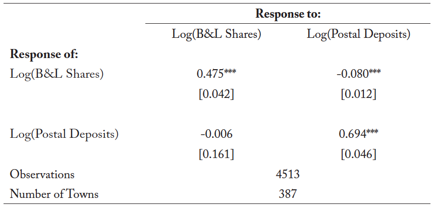
Notes: The table provides the results of a panel VAR regression. Each observation is a town-year. The sample contains all towns with at least one active B&L in a particular year. The two main variables are the logarithms of the vale of B&L shares and the value of postal savings deposits. All values are deflated to 1920 dollars. The regression includes both town and year fixed effects and the log of town population. Robust standard errors are presented in parentheses below the coefficients. * denotes significance at the 10% level, ** at 5%, and *** at 1%.

Table 2: Variance decomposition of postal savings and B&Ls: 1920–35

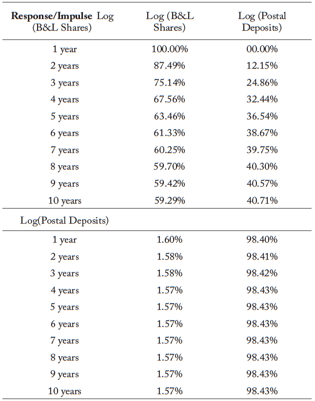
Notes: The table provides the variance decomposition of the panel VAR regression in table 1. The sample contains all towns with at least one active B&L in a particular year. Each observation is a town-year. The two main variables are the natural log of the number of B&L shares and the natural log of the value of postal savings deposits. The regression includes both town and year fixed effects and the log of town population.

Table 3: Panel VAR of postal savings and B&Ls, controlling for commercial banks: 1920–35

Notes: The table provides the results of a panel VAR regression. Each observation is a county-year. The sample contains all counties with at least one active B&L in a particular year. The two main variables are the logarithms of the number of B&L shares and the value of postal savings deposits. All values are deflated to 1920 dollars. The regression includes both county and year fixed effects, the log of county population, and the log of deposits at FDIC member banks. Robust standard errors are presented in parentheses below the coefficients. * denotes significance at the 10% level, ** at 5%, and *** at 1%.

Table A.1. Summary statistics

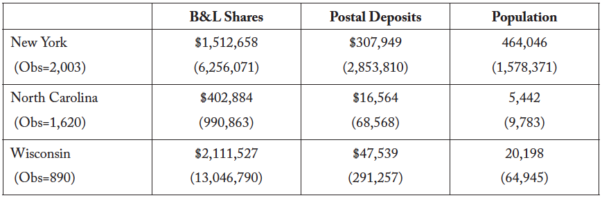
Notes: This table provides the town-level mean and standard deviations for our sample. B&L shares and postal deposits are deflated to 1920 values.

Figure 1: Postal Savings Deposits and B&L Shares: 1920–1940

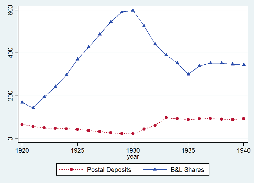
Notes: Figure provides the aggregate value of B&L shares and postal savings deposits in the three sample states. Values are deflated to 1920 values.

Figure 2: Locations of B&Ls (1920–1935)

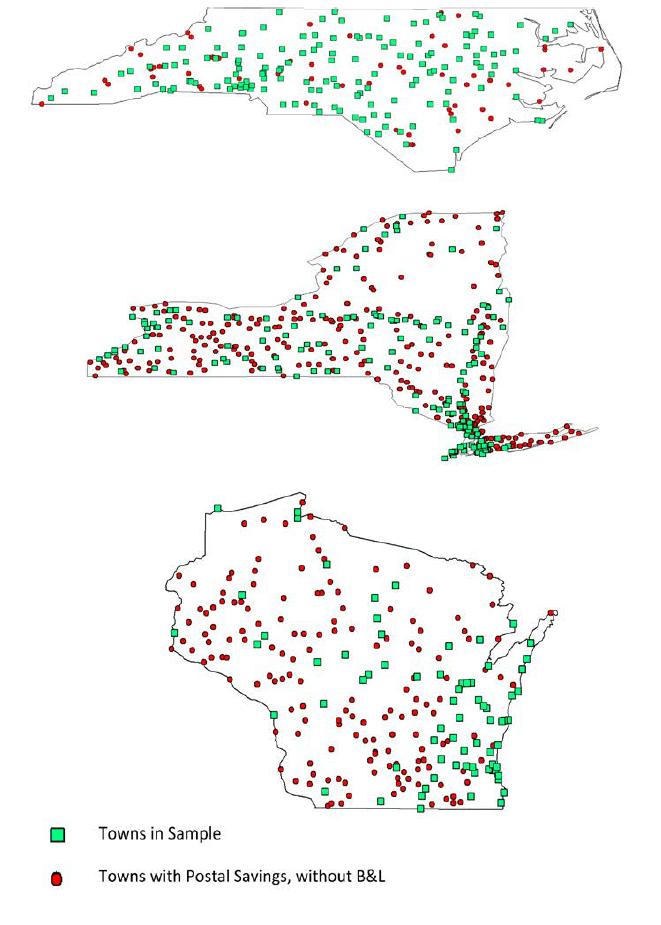
Notes: Figures map the locations based on the presence of a B&L. Locations denoted with squares have both a B&L and post office listed in the postal savings data (and are included in our sample), whereas locations with circles have only a listed post office (and are excluded from our sample).

Figure 3: Impulse Response Functions of Postal Savings and B&Ls: 1920–1935

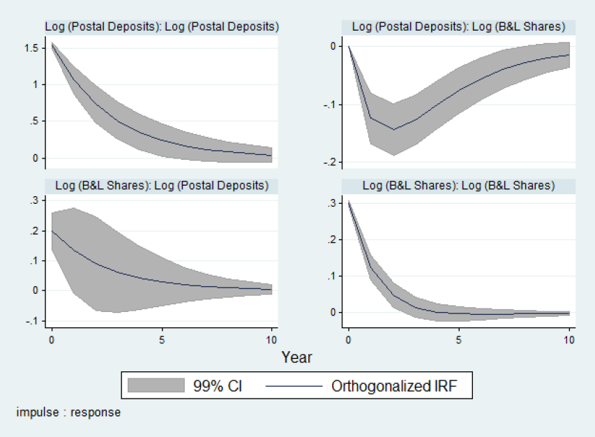
Notes: This figure provides the IRFs of the panel VAR regression in table 1. The sample contains all towns with at least one active B&L in a particular year. Each observation is a town-year. The two dependent variables are the natural log of the number of B&L shares and the natural log of the value of postal savings deposits. The regression includes both town and year fixed effects and the log of town population.

Figure A.1. Unit root tests

A1(i): Unit root test for regression results presented in table 1

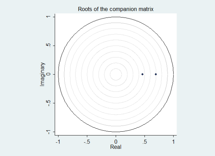
Figure A1(ii): Unit root test for regressions presented in table 3

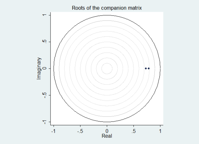
Note: Figures show the unit root tests for the regressions presented in this paper. These estimates were obtained using STATA’s pvarstable command, which calculates the modulus of each of the model’s eigenvalues. Figure A1(i) corresponds to the town-level regressions and A1(ii) to county-level regressions. Both tests show that the regression satisfies stationarity conditions.

References

Bodfish, H. 1931. History of Building and Loan in the United States. Chicago: United States Building and Loan League.
Bodfish, M. 1935. The Depression Experience of Savings and Loan Associations in the United States. Chicago: United States Building and Loan League.
Clark, H. F., and F. A. Chase. 1927. Elements of the Modern Building and Loan Associations. New York: Macmillan.
Courtemanche, C., and K. Snowden. 2011. “Repairing a Mortgage Crisis: HOLC Lending and Its Impact on Local Housing Markets.” Journal of Economic History 71 (2): 307–37.
Davidson, L., and C. D. Ramirez. 2016. “Does Deposit Insurance Promote Financial Depth? Evidence from the Postal Savings System during the 1920s.” GMU Working Paper no. 16-37.
Federal Deposit Insurance Corporation. Federal Deposit Insurance Corporation Data on Banks in the United States, 1920–1936. Ann Arbor, MI: Inter-university Consortium for Political and Social Research, 1992-02-16. https://doi.org/10.3886/ICPSR00007.v1.
Fleitas, S., P. Fishback, and K. Snowden. 2018. “Economic Crisis and the Demise of a Popular Contractu- al Form: Building & Loans in the 1930s.” Journal of Financial Intermediation 36: 28–44.
Fishback, P., S. Kantor, A. Flores-Lagunes, W. Horrace, and J. Treber. 2011. “The Influence of the Home Owners’ Loan Corporation on Housing Markets during the 1930s.” Review of Financial Studies 24 (6): 1782–1813.
Fishback, P., J. Rose, and K. Snowden. 2013. Well Worth Saving: How the New Deal Safeguarded Home Ownership. Chicago, IL: University of Chicago Press.
Fishback, P., S. Fleitas, J. Rose, and K. Snowden. 2019. “Collateral Damage: The Impact of Foreclosures on New Home Mortgage Lending in the 1930s.” NBER Working Paper 25246, National Bureau of Economic Research.
Gertler, M., and S. Gilchrist. 2018. “What Happened: Financial Factors in the Great Recession.” Journal of Economic Perspectives 32 (3): 3–30.
Jordà, Ò. 2005. “Estimation and Inference of Impulse Responses by Local Projections.” American Economic Review 95 (1): 161–82.
Kemmerer, E. 1917. “Six Years of Postal Savings in the United States.” American Economic Review 7 (1): 46–90.
Kendall, L. 1962. The Savings and Loan Business. Englewood Cliffs, NJ: Prentice-Hall.
Kilian, Lutz, and Yun Jung Kim. 2011. “How Reliable Are Local Projection Estimators of Impulse Re- sponses?” Review of Economics and Statistics 93 (4): 1460–66.
Kuwayama, P. 2000. “Postal Banking in the United States and Japan: A Comparative Analysis.” Monetary and Economic Studies 18 (1): 73–104.
Love, I., and L. Zicchino. 2006. “Financial Development and Dynamic Investment Behavior: Evidence from Panel VAR.” Quarterly Review of Economics and Finance 46 (2): 190–210.
Moen, J., and E. Tallman. 1992. “The Bank Panic of 1907: The Role of Trust Companies.” Journal of Economic History 52 (3): 611–30.
O’Hara, M., and D. Easley. 1979. “The Postal Savings System in the Depression.” Journal of Economic History 39 (3): 741–53.
Rose, J., and K. Snowden. 2013. “The New Deal and the Origins of the Modern American Real Estate Loan Contract.” Explorations in Economic History 50 (4): 548–66.
Rose, J. 2014. “The Prolonged Resolution of Troubled Real Estate Lenders during the 1930s.” In Housing and Mortgage Markets in Historical Perspective, edited by E. N. White, K. Snowden, and P. Fishback, 245–84. Chicago, IL: University of Chicago Press.
Schewe, D. 1971. A History of the Postal Savings System in America, 1910–1970. PhD diss., The Ohio State University.
Shoven, J., S. Smart, and J. Waldfogel. 1992. “Real Interest Rates and the Savings and Loan Crisis: The Moral Hazard Premium.” Journal of Economic Perspectives 6 (1): 155–67.
Sissman, L. 1936. “Development of the Postal Savings System.” Journal of the American Statistical Association 31 (196): 708–18.
Sprick Schuster, S., M. Jaremski, and E. Perlman. 2019. “An Empirical History of the United States Postal Savings System.” NBER Working Paper 25812, National Bureau of Economic Research.
Snowden, K. 2003. “The Transition from Building and Loan to Savings and Loan.” In Finance, Intermediaries and Economic Development, edited by S. Engerman, P. Hoffman, J. Rosenthal, and K. Sokoloff, 157–206. Cambridge: Cambridge University Press.
Snowden, K. 2010. “The Anatomy of a Residential Mortgage Crisis: A Look Back to the 1930s.” In The Panic of 2008: Causes, Consequences and Proposals for Reform, edited by L. Mitchell and A. Wilmarth, 51–76. Northampton, MA: Edward Elgar Publishing.
Snowden, K. 2014. “A Historiography of Early NBER Housing and Mortgage Research.” In Housing and Mortgage Markets in Historical Perspective, edited by E. N. White, K. Snowden, and P. Fishback, 15–38. Chicago: University of Chicago Press.
US Congress. 1931. Congressional Record.
Vossmeyer, A. 2016. “Sample Selection and Treatment Effect Estimation of Lender of Last Resort Policies.” Journal of Business and Economic Statistics 34 (2): 197–212.