The Costs of Building Walls: Immigration and the Fiscal Burden of Aging in Europe

Bernadino, Tiago; Franco, Francesco; Teles Morais, Luís

1 Introduction

Population aging is a major concern for developed economies, particularly in Europe. Over the last decades, fertility rates have fallen, and as life expectancy continues to rise, the population share of working-age individuals has shrunk. In Europe, the old-age dependency ratio – the ratio of the 65-plus to 20- to 64-year-old population – is projected to increase by more than 20 percentage points, from 34.8 percent in 2019 to 56.7 percent in 2050 (Eurostat, 2020). Absent any adjustment, these trends represent a burden for public finances – the fiscal burden of aging. Revenue from social security contributions and income taxes falls as the share of the working-age population decreases. At the same time, public spending grows, namely on retirement benefits and healthcare services, which are primarily consumed by the elderly.

Immigration often appears in public debate as a remedy for the fiscal burden of aging. Indeed, as Figure 1 shows, individuals immigrating to the European Union (EU) in 2019 were much younger than the existing resident population. Crucially, current immigration flows to Europe are much more concentrated in the working-age group than the resident population stock. By rejuvenating the population and enlarging the labor force, immigration could help relieve the fiscal burden of aging. Yet, political platforms that portray it as a problem are gaining more and more traction. As a result, many European countries are discussing policies to contain or even cut down immigration from the developing world.

Figure 1. Age Distribution of the Population Stock and the Immigration Flow to the EU in 2019

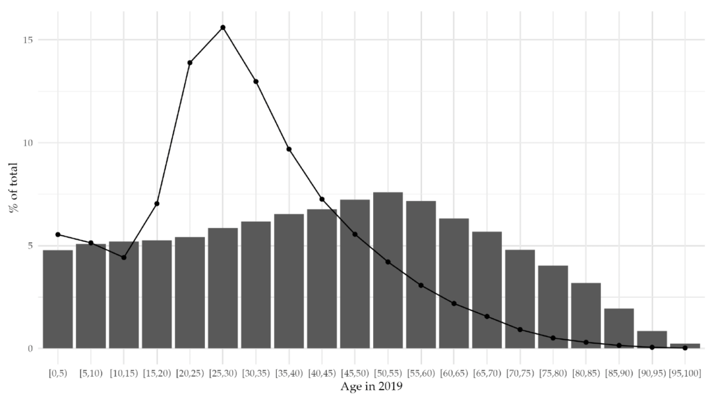
Note: Each gray bar represents the percentage of the resident population in the EU belonging to a specific age group in 2019. The solid black line represents the percentage of immigrants arriving in the EU from outside the union in 2019, also segmented by age group.

In this paper, we study the implications of changing migration inflows for public finances in the Euro area (EA). We find a nonlinear relationship between the size of immigration and its impact on public finances. Specifically, we find that while restricting immigration could increasingly strain public finances by exacerbating the age-dependency ratio, expanding immigration inflows yields diminishing returns for public finances and has a limited effect on altering the population’s age structure. This conclusion draws from a classic result in demographic modeling. In populations where native fertility rates are below the replacement level, like in much of Europe, immigration is vital: not only for stabilizing population dynamics and preventing its decline, but also for maintaining a balanced age-dependency ratio in the medium term.

Building on these theoretical insights, we explore the implications for public finances through an empirical application to present-day Europe. Using multiple survey data sources, we estimate demographic profiles of taxes and benefits segmented by age, gender, skill level, and country of birth, within the EA. We combine these data, covering the complete government budget, with customized population projections.

With these data, we measure the fiscal burden of aging. In line with the generational accounting tradition, we compute a counterfactual government budget series, by keeping the demographic profiles of taxes and benefits fixed and applying them to our population projections. The fiscal burden of aging is measured by calculating the net tax increase required to ensure public debt sustainability under this counterfactual budget. By producing this measure under different scenarios for migration, we trace out the role of immigration flows in mitigating the fiscal burden of aging.

As of 2019, the EA aggregate primary balance had a small deficit of 0.2 percent of the potential GDP, due to a positive net contribution from non-EU immigrants. Without their contribution, this small deficit would have been larger. Projecting into the future, if we held the current demographic profiles of taxes and benefits constant, with population aging as forecasted, the primary deficit would become 8 percent of potential GDP by 2060 and 9.6 percent by 2100. In this scenario, to ensure fiscal sustainability in the EA, the total tax burden would have to permanently increase by 15 percent across the EA.

These baseline results rely on sustaining the positive migration inflow of 2019 in the future, both in its overall size and current age-skill structure. In this year, the immigration inflow to the EA was about 1 percent of the population (i.e. around 3.34 million new immigrants). A decrease of this flow by 50 percent would cause the fiscal burden of aging to be much larger, necessitating a permanent tax increase of 16.3 percent to ensure fiscal balance. On the contrary, increasing the immigration flow by 50 percent would result in a 0.9 percentage point decrease in the rebalancing tax increase.

Restrictions on immigration from outside the EU have become a focus of political debate in many European countries. Our results highlight that policymakers considering such restrictions risk worsening the fiscal burden of aging for their constituents, because of the effects of immigration on demographic dynamics. Nevertheless, fostering immigration on its own cannot solve the fiscal gap caused by aging. We confirm this conclusion but add that this result is rooted in the nonlinearity that we uncover. We also show empirically that at the current levels of immigration in the EU, there is still room for gains from increasing immigration flows.We find a nonlinear relationship between the size of immigration flows and the rebalancing tax increase. The effects of reducing the immigration flow grow with the restriction’s size. Conversely, increasing the immigration flow has a decreasing beneficial impact on the rebalancing tax increase. These results are robust to different assumptions for the fertility rates of immigrants and their descendants, as well as for macroeconomic parameters. This nonlinearity has its roots in demographic dynamics, which generally apply to any population where fertility is below replacement and where there is a constant inflow of working-age immigrants.

Related literature and contribution The debate on the fiscal consequences of immigration, and its potential to relieve the fiscal burden of aging, is not new. Existing literature has been using three primary approaches to investigate this issue: fiscal accounting (both static and dynamic), general equilibrium models, and time-series models. In the first approach, and the one most used in the literature, static studies have calculated the costs and benefits of immigrants for public finances in a given year. A notable work in this area is by Dustmann and Frattini (2014), who estimated the impact of immigration on the United Kingdom economy between 1995 and 2011. However, immigration has a long-term impact on public finances as immigrants not only pay taxes but also have descendants who benefit from public education and will eventually benefit from retirement pensions.

As such, a dynamic approach that includes the dynamics of all benefits and contributions is more adequate. Auerbach and Oreopoulos (1999) is one of the first studies to adopt this approach. The authors estimate the fiscal contribution of immigration in the United States using net present value calculations. Subsequently, other papers have done the same for several European countries (Bonin et al. (2000) for Germany, Storesletten (2003) for Sweden, Collado et al. (2004) for Spain, Mayr (2005) for Austria, and Chojnicki (2013) for France). The consensus is that while increasing immigration may alleviate long-term fiscal imbalances, the quantitative impact is relatively modest. Preston (2014) provides an encompassing review.

Additional studies, such as Storesletten (2000) and Fehr et al. (2004), adopt the second methodology that uses general equilibrium models. These works consider the potential spillover effects of immigration on factors such as labor productivity and wages. They do not substantially alter the conclusions from the fiscal accounting papers strand, except for Hansen et al. (2017), who find that in Scandinavian-type welfare states, the effects of lower-skilled immigration on social transfer spending may be enough to overturn the positive effects of increasing young immigrant inflows.

A third different strand of studies such as D’Albis et al. (2019) and Furlanetto and Robstad (2019) addresses the issue using a vector autoregressive approach. Using a panel of OECD countries, they estimate the impact of well-identified immigration shocks on several macroeconomic variables, including public finances. They find evidence of a small, positive demographic dividend from immigration.

Our paper aligns with the first group of studies, investigating the contributions not only in a single year (static fiscal accounting) but also over the entire life cycle (dynamic fiscal accounting). Due to distinct hypotheses guiding budget projections, there are few comparable studies. One of our contributions to the literature is applying the same methodology to different countries and hence allowing cross-country comparisons. Furthermore, and more importantly, our paper is the first, to the best of our knowledge, to document the nonlinear fiscal contribution of immigration to public finances.

More recently, two papers have also sought to contribute to this literature by examining the whole EU, as we do. Using the static fiscal accounting approach, Fiorio et al. (2023) find that migrants had a positive net contribution to the EU budget between 2014 and 2018. Our paper sets itself apart by focusing on the dynamic fiscal accounting methodology, which we consider more relevant to answer this question. A second paper by Christl et al. (2022) moves toward a dynamic fiscal accounting approach, employing the projection model of Sutherland and Figari (2013) to estimate the net contributions of immigrants up to 2035. Our empirical analysis differs from this paper in three main aspects. First, it speaks to the effects on long-run demographic dynamics, considering the entire life cycle of migrants. Second, it simulates different levels of migration inflows in Europe, allowing us to derive our main result regarding the nonlinearity of the immigration effects on public finances. Last, it carefully estimates the demographic profiles of taxes and benefits that cover a larger part of the government budget and are consistent with national accounts.

In summary, our paper goes beyond simply demonstrating the positive net contribution of immigrants to the government budget. We reveal a nonlinear effect of altering immigration flows on the demographic dynamics of an aging population, along with the subsequent implications for public finances. We show that these effects are present in the results of this large literature on the fiscal impact of immigration.

Organization The rest of the paper is organized as follows. Section 2 describes the accounting methodology used to assess the impact of aging on public finance. Section 3 describes the data and some implementation details. Section 4 presents the budget balance decomposed by different demographic characteristics and our customized population projections. Section 5 describes the results on the role of migration in European public finances, and Section 6 concludes.

2 Measuring Intertemporal Fiscal Imbalances

Our methodology is based on the seminal work of Auerbach et al. (1991), who proposes generational accounting as a meaningful alternative to standard public accounts that consider how demography affects public finances. In this section, we show how to map the budget aggregates into different demographic groups to estimate the demographic profiles of the budget for each country in the EA. We also show how we build our customized population projections. We then compute the budget implied by these population projections, under the estimated demographic profiles. Last, we aggregate the budget across countries and derive an imbalance metric that corresponds to the permanent tax increase needed for the EA public finances to be sustainable.

2.1 Mapping Budget Aggregates to Demographic Groups

The government of country n faces a yearly nominal budget constraint, where government bonds at the end of a period are equal to the sum of the primary deficit with the government debt of the previous period plus the interest paid on that debt:

(1) $\begin{equation*}B_{t}=G_{t}-T_{t}+(1+i_{t})B_{t-1},\end{equation*}$

where $B_t$ is government debt in period $t$ , $G_t$ is total public expenditure net of interest payments on the outstanding debt in period $t$ , $T_t$ is total revenues received in period $t$ , and it is the implicit nominal interest rate paid on the debt during period $t$ . For simplicity of notation, we abstract from the country index, $n$ , unless it is fundamental for understanding.

Total revenues and expenditures are sums of different revenue categories, such as different types of taxes and social benefits, respectively. Each total is an aggregate of its respective categories. As we want to understand the impact of demographics on public finance, we map each budget category, $i$ , to a demographic group, $x$ . Government revenues in a year $t$ can be expressed as

(2) $\begin{equation*}T_{t}=\sum_{i}T_{t}^{i}=\sum_{i}\sum_{x\in X}\tau_{t,x}^{i} P_{t,x}, \end{equation*}$

where $\tau_{t,x}^{i}$ is the average per capita government revenue of category $i$ that is attributed to an individual of cohort $x$ in the year $t$ , and $P_{t,x}$ is the number of individuals of cohort $x$ alive in year $t$ . Similarly, government expenditures in a given period $t$ can be expressed as the sum of all expenditure items, $G_{t}^{i}$ , across all demographic groups:

(3) $\begin{equation*}G_{t}=\sum_{i}G_{t}^{i}=\sum_{i}\sum_{x\in X}g_{t,x}^{i}P_{t,x}, \end{equation*}$

where $g_{t,x}^{i}$ is the average per capita government expenditure of category $i$ attributed to a person of cohort $x$ in year $t$ . We refer to $\tau_{t,x}^{i}$ and $g_{t,x}^{i}$ as the demographic profile of revenue item $i$ and expenditure item $i$ , which correspond to the demographic structure of the government budget. In Section 3, we estimate them for the different EA countries using a combination of several microdata sources and macro aggregates.

2.2 Projecting toward the Future

To build a counterfactual path of the budget balance, we must project both total revenues and total expenditures over time. As shown in Equations (2) and (3), we need the population stock for each demographic group and the demographic profile of each budget item to compute the budget aggregates. In this subsection, we show how we project these two elements toward time for each EA country.

For the first element, the population stock, we combine projections for the fertility rate, the mortality rate, and net migration. While long-run population projections are readily available from several statistical institutions, they do not possess the granularity that we need for our exercise. We consider that a demographic group corresponds to people with the same age $a$ , gender $g$ , country of birth $c$ , and, as in Chojnicki and Rabesandratana (2018), skill level $k$ . We build our own projections using the cohort component method, which is standard in several demographic studies.¹ The population stock of a demographic group with age $a$ , gender $g$ , and country of birth $c$ evolves according to

(4) $\begin{equation*} P_{t,a,g,c}=\begin{cases} \begin{array}{cc} (1-m_{t-1,a,g,c})P_{t-1,a,g,c}+\bar{I}_{t,a,g,c}, & \forall a>0\\ \sum_{a,g,c}P_{t-1,a,g,c}f_{t-1,a,g,c}\lambda_{t}+\bar{I}_{t,a,g,c} & \text{for }a=0 \end{array} & \text{for }t>\bar{t} \end{cases} \end{equation*}$

where $m_{t,a,g,c}$ , $\bar{I}{t,a,g,c}$ , and $f{t,a,g,c}$ correspond to the mortality rate, the net migration, and the fertility rate at time $t$ of the population with characteristics $a,g$ and $c$ , respectively. $\lambda_{t}$ is the gender breakdown of newborns in period $t$ .² Afterward, we split each of these groups of the population by skill level, assuming that (i) for each individual, skill does not change after the age of 25 and (ii) the skill distribution observed at age 25 in the initial year is constant throughout time.³

For the second element, the demographic profiles, we set the growth rate of the path of nominal per capita revenue item $i$ , for each demographic group $x$ , to be the growth rate of the EA’s labor productivity, $\gamma$ , plus the EA inflation rate, $\pi$ :

(5) $\begin{equation*}\tau_{t,x}^{i}=\tau_{\bar{t},x}^{i}\prod_{j=\bar{t}+1}^{t}\left(1+\gamma_{j}\right)\left(1+\pi_{j}\right),\text{ for }t>\bar{t},\end{equation*}$

and mutatis mutandis for government expenditure items. This methodology allows us to project taxes and expenditures, for each country in the EA, throughout time.

2.3 Aggregation and Imbalance Metric

We next assess the implications of demography in the EA’s public finances. We take the projected government revenues and expenditures for the different countries of the EA and sum them to obtain the aggregated EA revenues and expenditures:

(6) $\begin{equation*}T_{t,EA}=\sum_{n\in EA}T_{t,n},\end{equation*}$

and similarly for the EA government expenditures, $G_{t,EA}$ .

Next, we derive a metric to measure the intertemporal fiscal imbalances. We assume that the current demographic structure of the budget in the EA does not change except in size. It is important to note that we do not aim to accurately forecast the different budget aggregates, whose future paths certainly depend on many factors beyond demographics. Our goal is to quantify the fiscal imbalances created by aging and, by changing the demographic projection, the role of migration in closing them.

Following the generational accounting literature, we define public finances to be balanced if the present discounted value of current and future revenues is equal to the present discounted value of current and future expenditures plus current debt, that is if the intertemporal government budget constraint (IGBC) holds. The IGBC is simply the sum, over infinite periods into the future, of the yearly budget constraint described in Equation (1), starting in the base year $\bar{t}$ :

(7) $\begin{equation*}\sum_{s=0}^{\infty}\prod_{j=1}^{s}\frac{G_{\bar{t}+s,EA}}{\left(1+i_{\bar{t}+j}\right)}-\sum_{s=0}^{\infty}\prod_{j=1}^{s}\frac{T_{\bar{t}+s,EA}}{\left(1+i_{\bar{t}+j}\right)}+B_{\bar{t}-1,EA}=\lim_{s\rightarrow\infty}\prod_{j=1}^{s}\frac{B_{\bar{t}+s,EA}}{\left(1+i_{\bar{t}+j}\right)}.\end{equation*}$

Let $D_{t}\equiv\frac{\left(1+\gamma_{t}\right)\left(1+\pi_{t}\right)}{1+i_{t}}$ represent a growth/discount factor, which we assume (for simplicity) is constant; that is, $D_{t}=D\;\forall t$ . Following our definition of balanced public finances, we must have the limit on the right-hand side of Equation (7) equal to zero and the equation to hold. The first condition corresponds to a no-Ponzi game condition; that is, the public debt is not on an exploding path. For the second condition to hold, we introduce a wedge, $(1+\theta_{\tau})$ , which corresponds to a proportional adjustment factor to revenues. Given a set of demographic profiles at $\bar{t}$ , future paths for the population of each country $n$ and each cohort $x$ , and a starting value for public debt $B_{\bar{t}-1}$ , we can derive the adjustment factor, $\theta_{\tau}$ :

(8) $\begin{equation*}\sum_{s=0}^{\infty}\sum_{n\in EA}\sum_{i}\sum_{x\in X}D^{s}\left[g_{\bar{t},n,x}^{i}-(1+\theta_{\tau})\tau_{\bar{t},n,x}^{i}\right]P_{\bar{t}+s,n,x}+B_{\bar{t}-1,EA}=0.\end{equation*}$

The adjustment factor $\theta_{\tau}$ represents the permanent increase, across all revenue categories, countries, and cohorts, necessary to ensure intertemporal fiscal balance, keeping the same demographic structure of the budget. We refer to $\theta_{\tau}$ as the rebalancing tax increase. Furthermore, given that this is an adjustment for all countries of the EA, the value of $\theta_{\tau}$ might imply cross-country redistribution. In other words, the surpluses of some countries might finance the deficits of other countries.

Before we proceed, let us discuss two technicalities of this adjustment factor. First, note that the same exercise could be performed by instead introducing an adjustment factor on government expenditure. This factor would represent the permanent change required in all expenditure categories to ensure the IBC holds. The results of doing so are symmetric, and therefore, for presentation purposes, we focus only on the rebalancing tax increase. Second, we are projecting the budget aggregates departing from a base year, $\bar{t}$ , that carries two year-specific effects: (i) effects associated with the particular histories of cohorts alive in $\bar{t}$ , such as wage trends or retirement choices, and (ii) business-cycle effects on the budget at $\bar{t}$ , such as higher unemployment benefits due to $\bar{t}$ being a recession year. To clean the latter effects, we use cyclical adjustments to fiscal aggregates, following the approach of Bonin et al. (2014), who apply the cyclically neutral budget adjustments of Girouard and André (2006) to a generational accounting exercise.⁴

For comparison purposes with other studies that have been done on the impact of demographics on public finance, we also report two other imbalance metrics. The first metric is the one used in traditional generational accounting studies following Auerbach et al. (1991) ( $\theta_{\tau}^{AGK}$ ), which distinguishes between presently living and unborn generations. This metric represents the permanent change in revenues solely attributable to future generations – the generation born after the base year – while taxes for current generations remain unchanged.⁵ The second measure commonly reported is the intertemporal budget gap ( $IBG$ ). This metric does not rely on a definition of intertemporal fiscal balance and instead simply sums the projected budget deficits, reported as a ratio to GDP in the initial period ( $Y_{\bar{t}}$ ). This metric provides insights into the size of future liabilities arising from aging.⁶ We show these two measures in Section 5, alongside the rebalancing tax increase.⁷

3 Data

In this section, we describe the data sources we use as well as the implementation details of the accounting methodology described in Section 2. With that, we estimate the demographic profiles of the different revenue and expenditure items and build our customized population projection for each EA country, by age, gender, skill level, and country of birth.

3.1 Data Sources

We must build two objects: the set of demographic profiles for various budget items for the universe of EA countries, and the demographic projections for each cohort $x$ for all EA countries. The first object requires individual micro-level data with the demographic characteristics of individuals, their contributions to each tax, and their benefits from each social subsidy and public service. Furthermore, we want our exercise to be consistent with the national accounts. As such, we need the macro-aggregate values of the different budget items. For the second object of the population projections, we need forecasts for fertility, mortality, and net migration by age, gender, and country of birth. Moreover, we also need to know the skill distribution for the initial period.

Individual microdata on taxes and benefits come mostly from the EU Statistics on Income and Living Conditions (EU-SILC) survey. This data set aims to collect timely and comparable cross-sectional and longitudinal data on income, poverty, social exclusion, and living conditions. We use cross-sectional individual data on labor income, income and property taxes, and social transfers, including pensions and demographic characteristics to estimate $\tau_{\bar{t},x}$ and $g_{\bar{t},x}$ . This covers most of the spending and revenue items that we map to different demographic characteristics.

To achieve a more complete coverage of the government budget, we use two additional microdata sources. We obtain household-level data on consumption from the Household Budget Survey (HBS), in order to derive the demographic profile of consumption, used to allocate value-added tax. We also use the European Central Bank’s Household Finance and Consumption Survey (HFCS) data on household business wealth holdings, which we take as a proxy measure for the incidence of corporate income tax.⁸

For healthcare spending, we obtain an age-gender profile of government health expenditure reported directly by the European Ageing Working Group (Aging-Working-Group, 2021). For education, we use data from Eurostat that report expenditures by level of studies. This allows us to map level of studies to an associated age group. Appendix D summarizes these different microdata sources.

Macrodata on public revenues and expenditures, as well as on government assets and liabilities, are retrieved from Eurostat. In all cases, we refer to data for the general government sector. For the interest rate, $i$ , we compute the historical average implicit rate from the outstanding stock of public debt. We also obtain data on labor productivity, to compute $\gamma$ , and on the inflation rate, to compute $\pi$ , using the time average from 1995.

Demographic data also come from Eurostat, where we obtain population breakdowns by skill and country of birth. Specifically, we use the EUROPOP2019 central projection to obtain forecasts for mortality and fertility rates (Eurostat, 2020).

3.2 Implementation

We choose 2019 as our base year, which corresponds to the year of the data where we estimate the demographic profiles as well as the starting year for the population projections. We choose this base year for two reasons. First, it is the latest complete year of data before the COVID-19 pandemic, and hence the data are not contaminated by effects specific to the health crisis, affecting both the life-cycle profiles of taxes and benefits and the demographic data. Second, it allows our exercise to be in sync with the starting year of the EUROPOP2019 population projections. Nevertheless, we conduct robustness checks for other choices of the base year. We perform our estimations for the 19 countries that were part of the EA in 2019.⁹

The methodology takes the total revenue and total expenditure and breaks it down into different budget categories. It then decomposes the value of each item by age, gender, skill, and birthplace. However, the breakdown cannot be performed for every item in the government budget, due to data limitations and conceptual reasons. Benefits from government activities such as defense, justice, or regulation do not vary among individuals, as they are a public good that, by definition, is nonexcludable. For these reasons, we distinguish mappable items from uniform items. For the first group of items, which covers roughly two-thirds of the government budget in 2019, we estimate the demographic profiles. This group consists of five taxes (personal income tax, corporate income tax, value-added tax, social security contributions, and property tax) and seven spending items (old-age pension, disability pension, survival pension, sickness allowance, unemployment subsidy, education services, and healthcare services). For the revenues of the second group, we uniformly distribute them to all individuals older than 18 years, and for the expenditures, we distribute them uniformly, independent of any demographic characteristic.¹⁰ In Appendix C.3 we describe the estimation of the different profiles.

In terms of demographic characteristics, our accounting framework considers ages between 0 and 100, where 100 corresponds to individuals who are 100 or more years of age, and two genders (male and female). Regarding skill level, we consider three different levels: skill level 1, which corresponds to having completed lower secondary education or below (ISCED 2 and below); skill level 2, which corresponds to having completed upper- and post-secondary education (ISCED 3 and 4); and skill level 3, which corresponds to having obtained a college degree (ISCED 5 and higher). Finally, we consider two groups in terms of birthplace: those born in the EU and those born outside the EU. Appendix C.4 describes how we build the population projections.

We assume that mortality rates are the same for individuals of the same age and gender living in the country. In other words, these rates do not vary across different skill levels or country of birth. For the fertility rate, we have different assumptions, dependent on the country of birth. For those born in the EU, we directly use Eurostat forecasts that project a slight increase in the fertility rate until 2100, but always below replacement. For those not born in the EU, we set a linear downward convergence path aiming to reach 2.1 by the year 2100. Furthermore, the second generation of immigrants has the same fertility rate as their parents.¹¹ Similarly to Section A, we set the immigration flow to be constant and equal to the value observed in 2019.

Furthermore, our accounting framework implies projecting the population toward a very distant future. In practice, we use the population laws of motion in the system of Equations (4) until 2100, and after that year, we assume a full stationary population distribution. This simplification, together with $D\in(-1,1)$ , implies that we can solve Equation (8) for the rebalancing tax increase, where the infinite sums are convergent geometric series.

4 Demographic Profiles and Population Projections

In this section, we discuss the estimation results of the demographic structure of the EA government budget primary balance of 2019. We also discuss the population projection that we use to forecast the counterfactual evolution of the primary balance and, ultimately, to assess the role of immigration in the public finances balance.

4.1 Primary Balance Decomposition

Using the microdata sources described in Section 3, we estimate the tax and benefit distribution by age, gender, skill level, and country of birth, for each country in the EA. We sum these objects across countries, following Equation (6), to have the demographic structure of the EA government budget for the base year, 2019.

This structure is also interesting per se. It allows us to know, for example, how much a 45-year-old man born outside the EA with a high school degree, on average, pays on personal income tax in the base year. Moreover, it allows us to decompose the base year’s primary balance by the different demographic characteristics, that is, age, gender, skill level, and country of birth. Figure 2 shows that decomposition.¹²

Figure 2. Decomposition of the EA Primary Balance for the Base Year, 2019

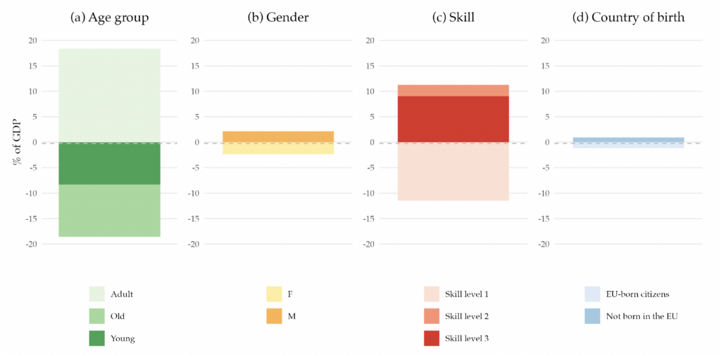
Note: The figure presents the decomposition of the EA primary balance by demographic characteristics. It represents the sum of revenues, net of benefits, attributable to individuals with specific demographic characteristics, expressed as a percentage of the 2019 potential GDP. The dashed line denotes the 2019 value of the primary balance (-0.2 percent). All values are shown as a percentage of the potential GDP.

When we decompose the primary balance by age groups, we find that the young and the elderly populations are net receivers of the government budget, while the working-age population is a net contributor to the budget. Their contribution rises to more than 15 percent of the GDP. This pattern can be easily understood when we think about the life-cycle dynamics regarding taxes and social benefits. The young generation benefits almost exclusively from education expenditure, as they only start paying taxes when they enter the labor market, which for most people is in their 20s. Hence, their net contribution to the primary balance is negative. Although they pay some taxes, the older generation is a net receiver from the government budget due to the social benefits they receive, namely retirement pensions and healthcare. Finally, the adult population receives very little social benefits, except occasionally for events such as unemployment or sickness. However, they are the biggest taxpayers since income and consumption peak during the working years, making them net contributors to the government budget.

Examining the gender decomposition, we find that men are net contributors to the budget, whereas women are net receivers. This disparity arises for a few reasons. While education is the same for the two genders, the taxes paid are different due to the variations in income received. These variations may be due to differences in labor market participation rate or differences in salaries across genders. Furthermore, due to their longer life expectancy, women receive pension benefits and use healthcare services for a longer period compared to men.

Regarding the skill decomposition, individuals with lower skills have a net negative contribution to the budget. In contrast, those with skill levels 2 and 3 contribute positively yet not enough to achieve an overall positive primary balance. The underlying reason is similar to the male-female dichotomy: lower skills, means, on average, lower income, leading to lower tax contributions.

More relevant to our research question is the decomposition by country of birth. We find that those not born in the EU have a small but positive contribution, while EU-born individuals are net receivers of the public budget. This fact is linked to the younger age profile of immigrants, as shown in Figure 1. In 2019, immigrants already have a positive contribution to public finances as their absence would have resulted in a more negative primary balance.

4.2 Demographic Projections

As described in Section 2, a key object for our exercise is the detailed population forecast that will be used to project the government balance. For each country in the EA, we project the population stock by age, gender, country of birth, and skill level according to Equation (4), until 2100. After that year, we assume a full stationary population. Figure 3 plots, for selected years of the projection, the implied EA age, gender, skill level, and country of birth distribution. Our population projections imply that the population will age. The dependency ratio (the ratio of the young and old populations to the adult population) increases from 0.89 in 2020 to 1.13 by 2100. Panel (a) shows that the share of the adult population decreases, while the share of the old population increases. The share of the young population first decreases, due to the low fertility rates, but then slowly recovers to its initial value as fertility slowly rises. The gender distribution, represented in panel (b), is projected to remain constant, with the female population making up slightly half of the total population.

Our demographic forecasts imply the skill distribution of the adult population will change, as panel (c) illustrates. The highest skill level is expected to increase by 12 percentage points, whereas the lowest will fall by about 10 percentage points, between 2020 and 2100. Last, panel (d) shows that the share of non-EU immigrants is projected to rise from 10 percent of the adult population to 26 percent. The children of this part of the population, which has a higher fertility rate, are projected to represent 25 percent of the adult population in 2100.

Figure 3. Demographic Distributions Implied by the Population Projections

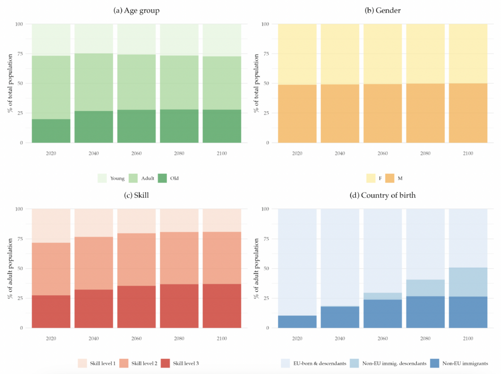
Note: The figure shows the percentage of people with given demographic characteristics. Panel (a) displays the age distribution by age group (young, adults, and old age). Panel (b) shows the gender distribution (female and male). Panel (c) presents the skill-level distribution as a percentage of the adult population, where skill level 1 corresponds to those who did not complete high school, skill level 2 corresponds to those who completed high school, and skill level 3 corresponds to those who completed college. Panel (d) depicts the distribution of country of birth as a percentage of the adult population.

5 Immigration and Public Finance Sustainability

In this section, we examine our counterfactual government budget implied by the population projection. We first use it to compute the rebalancing tax increase previously defined in Section 2, and examine the contributions of the different age and country of birth groups over time. We then present our main results on the impact of changing the immigration inflow in the EA on public finances. The section closes with a list of robustness exercises that we perform.

5.1 The Fiscal Burden of Aging

As described in Section 4, demographic projections until 2100 show that the population of the EA will age, with the dependency ratio increasing substantially. Other things equal, this trend is likely to put pressure on the sustainability of public finances. To quantify this fiscal burden of aging, we build the counterfactual government budget under our customized population projections, keeping fixed the demographic profiles of the different budget items.

In Figure 4 we plot the resulting primary balances, for selected years of the projection. The current deficit of 0.2 percent of the GDP in 2019 widens over time. By 2040, the primary deficit would be 5.1 percent, and by 2100, it would be almost 10 percent of potential GDP. This transformation of the primary balance into a permanent deficit is robust to the starting point, as the same trend is observed for individual EA countries. See Appendix F for the projected primary balance of each country.

Figure 4. Counterfactual Primary Balance Implied by the Population Projections Decomposed by Age Group and Country of Birth

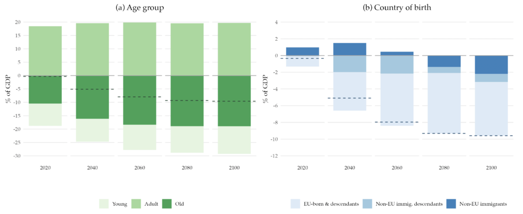
Note: The dashed lines in the figure represent the primary balance for selected years of the projection. Panel (a) shows the decomposition of the primary balance by age group (young: 0–24 years old; adult: 25–65 years old; and old: more than 65 years old). Panel (b) shows the decomposition of the primary balance by country of birth. All values are shown as a percentage of the potential GDP.

Under this counterfactual budget, by how much would the government need to increase taxes to rebalance public finances? To answer this question, we look at our rebalancing tax increase, $\theta_{\tau}$ , derived in Section 2, which is the increase necessary to ensure the IGBC holds. Table 1 shows this metric, together with two others: $\theta_{\tau}^{AGK}$ , a similar metric but considers the tax increase is only imposed on future generations, and $IBG$ , the intertemporal budget gap.¹³ Governments across the EA would need to increase taxes by 15 percent, for everyone and permanently. If instead they only put the burden on the generations born after 2019, then they would need to raise taxes by almost 30 percent.¹⁴

We now examine the contributions to the overall balance by different age and country of birth groups.¹⁵ Panel (a) of Figure 2 shows, for selected years, the decomposition of the primary balance by age group. As the dependency ratio rises, the negative contribution of the elderly population becomes larger, increasing from around 10 percent of GDP in 2019 to almost 20 percent of GDP in The young generations’ negative contribution is relatively stable throughout the projection time, with a slight increase in the later years. Similarly, the positive contribution from the adult population is close to 18 percent in 2020 and remains stable for most of the projection.

Panel (b) of Figure 4 decomposes the projected primary balance by country of birth. The negative net contribution from EU-born citizens and their descendants is projected to widen. Furthermore, while the immigrant group initially has a positive net contribution, after 2060, it also becomes a net receiver. This is due to the life-cycle effects that also occur in this case: when these individuals immigrate, they are mostly at working age and hence are contributing positively to the government budget. Eventually, they will also retire, becoming net receivers. As a whole, the immigrant group is also aging, which is not compensated by the relatively younger new immigration flow, nor by the return migration of non-EU-born individuals at older ages.

Throughout the projection horizon, the descendants of immigrants have a negative contribution. This negative contribution comes from the age composition and the life-cycle net contribution pattern of this subpopulation.¹⁶ In the first years of the projection, they are mostly benefiting from the education services provided by the government and hence have a negative contribution. This negative contribution decreases as they start entering the labor market but never reaches a positive value. In the later years of the projection, it increases as the older members of this group start to enter into retirement ages. This sets the baseline scenario of what aging would imply for public finances. Next, we analyze the extent to which immigration can help solve the fiscal burden that aging creates.

5.2 The Nonlinear Effects of Immigration on Public Finances

Immigrants from outside the EU currently have a positive contribution to the budget. In our baseline projection, this contribution turns negative, as they are subject to the same aging trends as natives. This decomposition does not, however, speak to the effect that the size of immigration flows has on fiscal aggregates. We turn to this issue in this subsection by running different population projections with different immigration flow sizes.

Our baseline projection assumes a constant net migration flow each year at the level observed in 2019, which constitutes around 1 percent of the 2019 EA population. We now explore various scenarios by considering different levels of net migration flow—multiples of the 2019 observed level– such that we have percentage increases and reductions of this flow. These transformations do not modify the age/gender/skill distribution of migration, only the total size of the net migration flow.¹⁷ This exercise is equivalent to what we do in the stylized demographic model of Appendix A, where we simulate the demographic transition for different constant migration flows.

We start by looking at the primary government budget balance under the different migration scenarios. The left panel of Figure 5 plots the counterfactual path of the primary deficit in these different scenarios. Regardless of the migration level, the current small primary deficit is anticipated to increase and stabilize around the year 2080. Our results show that immigration and public finance performance have a positive relation. A reduction in migration leads to a larger primary deficit, while an increase results in smaller deficits. This result aligns with other studies showing that immigration cannot fully solve the public finance sustainability issue faced by developed economies (Preston, 2014).

Figure 5. Primary Balance and the Age-Dependency Ratio under Different Net Migration Scenarios

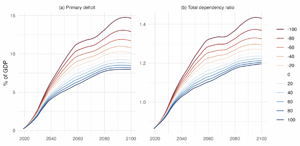
Note: Panel (a) shows the projected primary balance deficit as a percentage of the potential GDP for the different net migration scenarios. Panel (b) plots the total age-dependency ratio (computed as the sum of the young and the old populations divided by the working-age population) for these same migration scenarios.

Notably, the relationship between immigration size and the primary deficit is not linear. Instead, there is a uniform convergence pattern of the primary deficit as the immigration flows into Europe increase. Conversely, constraining migration has an increasing effect on the primary deficit; that is, reducing immigration is linked to growing costs for public finances. This observed pattern is connected to the dynamics of the dependency ratio in the population projections, as evident in the comparison of both panels in Figure 5.

Figure 6 illustrates the connection between immigration flow levels and the dependency ratio for selected years. The figure reveals a convex relationship, implying a diminishing impact of immigration on the dependency ratio, or conversely, increasing costs for the dependency ratio with immigration restrictions.¹⁸

Figure 6. Age-Dependency Ratio under Different Net Migration Scenarios

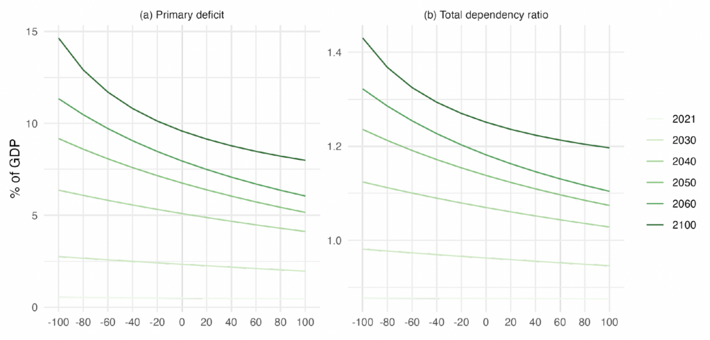
Note: Panel (a) shows the projected primary balance deficit as a percentage of the potential GDP for the different net migration scenarios. Panel (b) plots the total age-dependency ratio (computed as the sum of the young and the old populations divided by the working-age population) for these same migration scenarios.

Given the different paths for the primary balance implied by the population's age structure, let us now compute the corresponding rebalancing tax increase measure, $\theta_{\tau}$ , implied by the different values for the net migration flow. Figure 7 draws the frontier between the change in the migration flow and $\theta_{\tau}$ . Consistent with the patterns in the primary balance projection, the tax adjustment necessary to restore sustainability increases if migration flows are reduced. The difference is substantial: if immigration from non-EU countries is completely shut down, the rebalancing tax increase widens by a quarter, from 15 to 18 percent. Without immigrants coming in, the fiscal burden of aging becomes far heavier. For comparison, the metric $\theta_{\tau}^{AGK}$ , without migration flows, would rise from 29.9 to 46.3 percent.

Moreover, as the plot clearly shows, the relationship between immigration and the fiscal burden of aging is not linear but rather convex. Each marginal reduction of the migration flow has an increasing cost for public finances. In the case of the EA, this convexity matters quantitatively. Notice that if, hypothetically, immigration flows doubled in size, the rebalancing tax adjustment would decrease by only 1.5 percentage points. These gains are smaller, by about half than the costs of shutting down migration, meaning immigration cannot per se eliminate the fiscal burden of aging. In this sense, there are diminishing returns to increasing immigration on public finances. Nevertheless, even at the current level of immigration, Europe has not reached a point where it experiences no benefits from immigration in terms of public finances.

Figure 7. Frontier between the Level of Immigration and the Rebalancing Tax Increase Implied, $\theta_{\tau}$

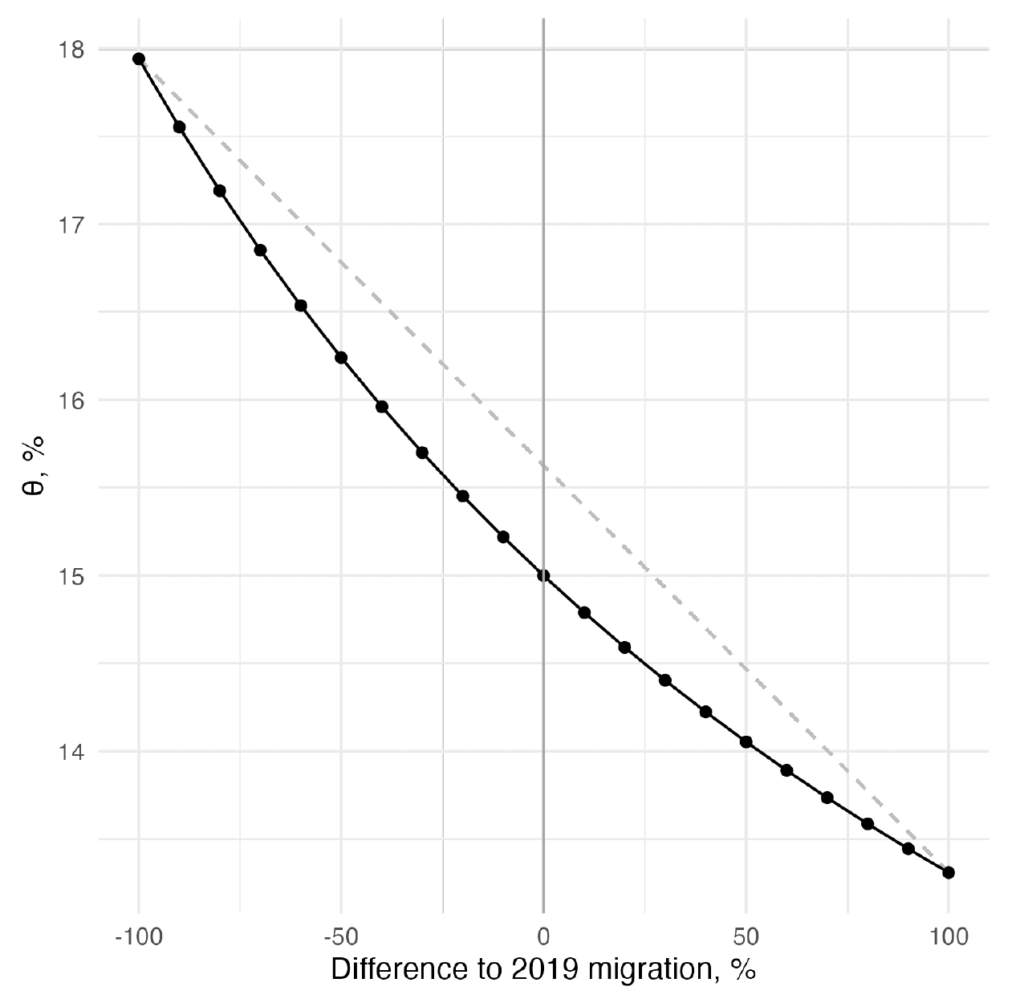
Note: The figure shows the $\theta_{\tau}$ value implied by different immigration scenarios. $\theta_{\tau}$ is computed according to Equation (8). The dashed line is an auxiliary straight line connecting the two extremes.

This convexity comes as a direct consequence of demographic dynamics presented in the stylized demographic model in Appendix A. In that model, this convexity emerges in the effects of immigration flows on the dependency ratio during the transition. We have shown that this carries through to a full, detailed demographic model, with information on the age, gender, and skill profiles of immigrants, and maps into the budget deficit using the demographic profiles of taxes and benefits in the data. To the best of our knowledge, this is a new result in the literature measuring the effects of immigration on public finances in developed countries.

5.3 Rebalancing Tax Increases at the Country Level

Our results, namely our headline imbalance metric $\theta_{\tau}$ , assume there is a common EA budget. This metric provides a summary of the situation at the European level, which is very heterogeneous across countries. Although the dependency ratio has been increasing in all EA countries and is projected to continue to do so, there are substantial differences within the EA. Spain has a dependency ratio of 0.52 dependents per working-age person, whereas France has a dependency ratio of 0.64. The demographic trends are also heterogeneous, with countries projected to have higher fertility rates than others.

With these different aging trends, the sustainability of the public finance situation is also quite heterogeneous. In Table 2, we compute the country-specific rebalancing tax increase under different migration scenarios. The baseline column shows the implied rebalancing tax increase under the observed 2019 migration scenario, allowing us to see which countries face a heavier fiscal burden of aging. Slovakia and Spain have the most unbalanced public finance situation and would need a permanent increase in taxes of 24 percent and 26 percent, respectively. On the other hand, Cyprus and the Netherlands are among the countries with the smallest rebalancing tax increase metric. Given this wide heterogeneity across countries, our main results, by assuming a common EA budget, might imply substantial fiscal redistribution. Countries whose budgets are more robust to aging would need to support those facing a higher fiscal burden of aging.

The table also shows the rebalancing tax increase for the two most extreme scenarios of migration that we consider in our exercise: one where all migrant flows are shut down, and another where migration is doubled compared to the baseline. By comparing them with the baseline, we can see to which countries migration flows are (or can be) more important. Portugal would be the most severely affected in terms of public finance sustainability if immigration flows were shut down, with the rebalancing tax increase rising by 7 percentage points. For other countries, the impact of immigration is smaller. This is due to the age structure of immigrants in each country and the point along the frontier between the flow size and $\theta_{\tau}$ , as determined by the country’s baseline proximity to a flat area (either closer or further away).

One of the contributions of our paper is providing and applying a common methodology to measure the fiscal imbalances brought by aging and the role that migration can have in minimizing it in different countries. Given the amount of data necessary to do this exercise and the different hypotheses that the methodology needs, there are not many papers that offer reasonable comparisons across countries.¹⁹

5.4 Robustness Exercises

Interest rate and productivity growth rate. In our baseline exercise, we set the demographic profile growth rate, $\gamma$ , the nominal interest rate, $i$ , and the inflation rate, $\pi$ , to the historical average of these variables between 1995 and 2021, that is, 0.7 percent, 3.8 percent, and 1.68 percent, respectively. This implies a discount factor, $D$ , equal to $0.986$ . Our result of increasing costs of reducing migration flows to public finance sustainability does not depend on the discounting effect. In fact, the metric for the rebalancing tax increase changes very little when we choose other values for $D$ . This becomes evident when solving Equation (8) for $\theta_{\tau}$ , which yields a ratio between expenditures and debt, and revenues. Since the debt's value is much smaller compared to the size of the present discounted value of the stream of revenues and expenditures, changing $D$ increases both the numerator and the denominator essentially in the same proportion. In Appendix E.1, we compute $\theta_{\tau}$ and plot the frontier between the level of migration and the imbalance factor, for different values of $D$ .

Fertility rate of immigrants. In our baseline scenario and in the different migration levels examined in the previous section, we take the fertility rate of the population born outside the EU in 2019 and assume a convergent path toward 2.1 children per woman by 2100. The choice for this path, arguably, could have an impact on the size of the immigrant population and consequently on the fiscal benefits that migration brings. However, our results are robust to this hypothesis. Changing the fertility path only slightly affects the value of the rebalancing tax increase metric and does not change the convex relationship between migration and this metric. In Appendix E.2, we compute $\theta_{\tau}$ for different assumptions of the fertility rate of the immigrants as well as the frontier between the imbalance factor and the level of migration.

6 Conclusion

Many European countries have been experiencing an increase in political polarization, and migration policy has played a central role in that trend. Notably, immigration from developing countries has become a contentious issue. In this study, based on detailed data on taxes, benefits, and demographic dynamics, we revisited the question of how immigration can help relieve the fiscal burden of aging. Our analysis uncovers a novel fact, informing both policy discussions and future research on immigration and public finance. Immigration has a positive, nonlinear effect on public finances. This indicates that restricting migration has increasing costs for public finances and, at the same time, that immigration alone cannot solve the fiscal burden of aging.

To arrive at this result, we first show that immigrants currently have a positive contribution to the government budget. Without them, the primary balance would be even more negative. Other things equal, the projected demographic trends in Europe bring the primary balance down to a large – and permanent – deficit within a few decades. With the same demographic profiles (by age, gender and education level) of the different budget items, sustainable public finances would require a permanent tax increase of 15 percent for everyone across the EA. The migration flows embedded in our population projections play a significant role in this result: without them, the necessary permanent tax increase would be about 3 percentage points higher. Conversely, doubling the migration inflows would only make the permanent tax increase be 1.5 percentage points lower.

Additionally, by applying a common methodology to different European countries, this paper provides a cross-country comparison of the impact of migration on public finances. These results are relevant for European policymakers considering restrictions on immigration from the developing world. Due to the effects of immigration on demographic dynamics, reducing immigration could significantly exacerbate the fiscal burden of aging.

Appendix

A Theoretical Background

In this appendix, we build a simple stylized demographic model that explains the demographic result that the immigration size has a nonlinear effect on the age-dependency ratio. This simple model allows us to trace out the same population dynamics that are present in the projections underlying our empirical exercise but in a simplified structure that allows us to understand them better. We start by describing the model, which is a stylized representation of the population dynamics. We then describe some properties of the model’s steady state. Finally, we show, with simulation, how migration affects the dependency ratio during the demographic transition.

A.1 Setup

The model structure aims to capture the essential features present in current European population dynamics. The population $P$ is composed in each period of three generations, the young generation $P_{y}$ , the adult generation $P_{a}$ , and the old $P_{o}$ . The adult generation is characterized by the ability to have children. Immigrants enter the population as adults, capturing the feature of the data that most immigrants from outside the EU are of working age.²⁰ The adult population is further split into $P_{a}^{F}$ , foreign adult population, and $P_{a}^{N}$ , native adult population. There is an exogenous flow of immigrants, a constant absolute value $M$ , in keeping with the most common assumption in the demographic literature and indeed in official population projections.

The fertility of immigrants $f^{f}$ may potentially differ from the fertility of natives $f^{N}$ , as in the data. The children of immigrants enter the native young population. The population stock of each group evolves according to the following system of difference equations:

(9) $\begin{equation*} \begin{aligned} & P_{o, t}=\left(1-\pi_m\right) P_{o, t-1}+\pi_o\left(P_{a, t-1}^N+P_{a, t-1}^F\right), \\ & P_{a, t}^N=\left(1-\pi_o\right) P_{a, t-1}^N+\pi_a P_{y, t-1}, \\ & P_{a, t}^F=\left(1-\pi_o\right) P_{a, t-1}^F+M, \\ & P_{y, t}=\left(1-\pi_a\right) P_{y, t-1}+f^N P_{a, t-1}^N+f^F P_{a, t-1}^F . \end{aligned} \end{equation*}$

Each period, the old face a certain probability $\pi_{m}$ of death (mortality rate), adults (both foreign and native) enter retirement with a probability $\pi_{o}$ , and young people enter adulthood with a probability $\pi_{a}$ . The Markov chain structure allows us to capture the key features of the life cycle: a certain time spent in infancy before becoming fertile and productive, and aging, where after some time individuals are no longer fertile and productive and enter a stage in which they face some likelihood of death. This model has two simplifying assumptions. First, there is no distinction between ages within groups, so for a given individual, the expected time spent in each age group will be counterfactual to the data. Second, non-old people have zero likelihood of death. These assumptions do not influence any of the results we highlight here.

This stylized model captures all the main features of the demographic dynamics present in our empirical exercise and, in fact, in most demographic projections, including official scenarios such as those produced by Eurostat.

A.2 Stable Population Results

We begin by highlighting in our framework some stable population results well-known in the demography literature (Schmertmann (1992) provides a summary of these results). When discussing results related to the population’s age structure, our focus will be on the total dependency ratio, which is defined as the ratio of the nonworking-age population (young and old) to the working-age population (adults). This measure is particularly pertinent for fiscal considerations as it provides a good approximation of the ratio of net beneficiaries from the government budget per net contributor.

Stationary through immigration. When native fertility rates are below replacement, this model gives rise to a long-run solution characterized by a stationary population, with a fixed age structure and population size (i.e., a population growth rate of zero). This stationary population consists, in essence, of immigrants and their descendants. The size of the immigration flow will be important in determining the stationary population’s size but not its age structure. If immigrants’ fertility is higher than that of natives, this will affect the age structure of the stationary population, but not the overall conclusion, as long as immigrants’ children revert to native fertility.²¹ We therefore focus on the simplest case of $f^{F}=f^{N}\equiv f$ in the ensuing discussion, and show in Appendix ?? that the results carry through to the case $f^{F}>f^{N}$ .

This can be easily seen by casting the model in state space form:

(10) $\begin{equation*}\textbf{P}{t}=A\textbf{P}{t-1}+B,\end{equation*}$

where $\textbf{P}{t}=\left[\begin{array}{ccc} P{o,t} & P_{a,t} & P_{y,t}\end{array}\right]'$ , $B=\left[\begin{array}{ccc}0 & M & 0\end{array}\right]'$ , and

$A=\left[\begin{array}{ccc} 1-\pi_{-} & \pi_o & 0 \\ 0 & 1-\pi_o & \pi_a \\ 0 & f & 1-\pi_a \end{array}\right]$

All of the eigenvalues of A are inside the unit circle given our parameter definitions and in the case of fertility below replacement ( $f<\pi_{0}$ ). This means $I-A$ is invertible, so we can solve the model backward, computing

(11) $\begin{equation*}\textbf{P}{t}=A^{t}\textbf{P}{0}+(I-A)^{-1}(I-A^{t})B.\end{equation*}$

The stationary population is then given by

(12) $\begin{equation*} \begin{aligned}\lim_{t\rightarrow\infty}\textbf{P}_{t}\equiv\textbf{P} & =(I-A)^{-1}B\\ \textbf{P} & =M\times\frac{1}{\pi_{\mathrm{o}}-\mathrm{f}}\times\left[\begin{gathered}\frac{\pi_{\mathrm{o}}}{\pi_{\mathrm{m}}}\\ 1\\ \frac{\mathrm{f}}{\pi_{\mathrm{a}}} \end{gathered} \right]. \end{aligned} \end{equation*}$

This equation makes it clear that the immigration flow’s size only matters for determining the scale of the stationary population and not its age structure.²² In the stationary population, the total dependency ratio is given directly by $\frac{f}{\pi_{a}}+\frac{\pi_{o}}{\pi_{m}}$ , which does not depend on $M$ , although it does depend on other parameters. The dependency ratio increases in $f$ (there will be a higher share of children) and in $\pi_{o}$ , as the ratio of time spent in old age to adulthood increases, increasing the share of the old population. It decreases in $\pi_{m}$ (higher mortality means lower life expectancy and time spent in old age, reducing the share of the old population) and in $\pi_{a}$ , as children becoming adults faster means a lower share of the young population.

Population dynamics of this kind are often called “stationary through immigration” or “SI” in the demography literature. All population projections for advanced economies incur this kind of dynamics, and the demographic dynamics that we have in our empirical section are no exception.

Extinction without immigration. Without immigration (i.e., $M = 0$ ), there is still a stable population, with constant population growth and a fixed age structure. However, in this case, as native fertility rates are below replacement, in the long run total population becomes zero, or, in demographic terms, faces extinction.²³ In this model, this stable population is characterized by a negative growth rate given by the largest eigenvalue of $A$ (Coale, 1986). The dependency ratio becomes a more complicated combination of parameters, which we numerically show next that, under a realistic calibration, gives a higher value than in the case of a population with a migration inflow.

A.3 Transitional Dynamics

Given any initial population, with positive migration inflows, the model's long-run solution will be given by Equation (12), the first case above. If $M$ is set to zero, we are instead at the second case. Importantly for our purposes, there is one single long-run dependency ratio for any $M>0$ , and another, higher, in the case of $M=0$ .

In the transition to those long-run solutions from some initial population, matters are different. In particular, the relevant case considering the data in most European countries is marked by an initial dependency ratio markedly lower than the corresponding stationary solution (an aging population). In this case, we will observe that as $M\rightarrow0$ , the dependency ratio in the transition becomes closer to the path associated with the extinction case and takes many periods to latch on to a different path, taking it to the stationary SI solution. For higher values of $M$ , the transition path is, from the outset, clearly different and associated with its final stationary state.

We provide an example of this by simulating the model above. The calibration does not intend to reproduce any specific country but reflects the fact that as observed in most European countries, the fertility rate of native adults is below replacement, while that of foreign adults is above replacement.²⁴ We set the initial values of the age group shares to match the shares observed in the EA in 2021 such that the initial dependency ratio is 57 percent.

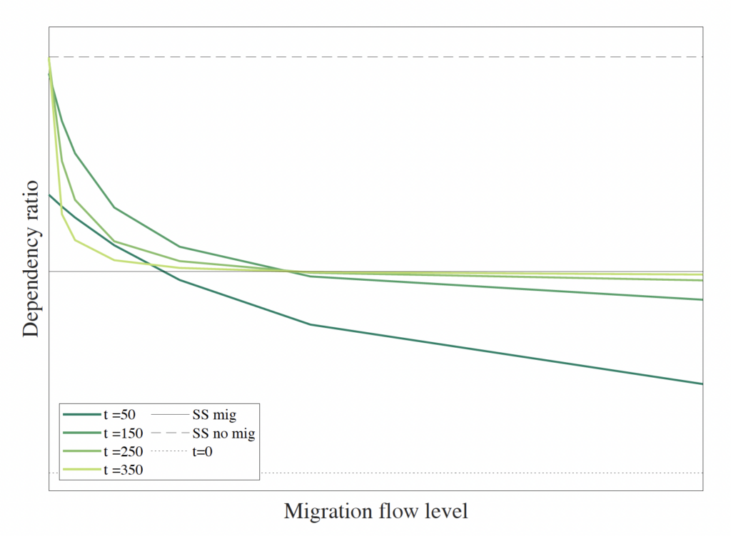
We examine the transition of the dependency ratio under different values for the size of the immigration flow, between 0 and 10 percent of the initial population (0, 0.1 percent, 0.2 percent, 0.5 percent, 1 percent, 2 percent, 5 percent, 10 percent). Figure A.1 plots the value of the dependency ratio along the transition for the different scenarios.

Figure A.1. Total Dependency Ratio Along the Demographic Transition

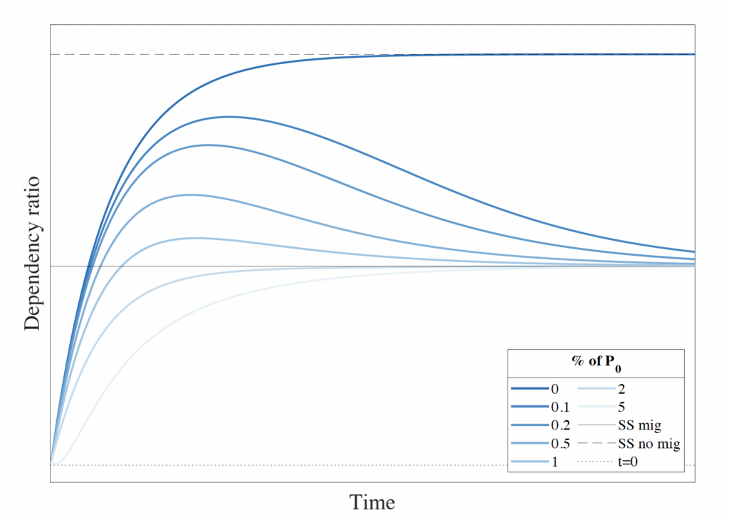
Note: The total dependency ratio is the quotient between the young and old populations over the adult population. The figure plots this ratio for different scenarios of an immigration reduction along the first 500 periods of the demographic transition to the steady state.

The model simulation produces an age distribution throughout the transition, demonstrating a convergence pattern to the stationary dependency ratio value of 1.17 for all positive values of immigration. However, this value is only attained after several hundred periods, illustrating that the immigration flow’s size has no impact on the age structure of the SI, as shown before.

Nevertheless, immigration does impact the age distribution during the demographic transition toward the stationary population. A smaller immigration flow leads to higher dependency ratios. As the dependency ratio serves as a concise representation of the fiscal burden of aging, higher ratios are associated with increased deficits, indicating a larger fiscal burden of aging. This aligns with established findings that immigration can alleviate long-term fiscal imbalances, as shown by studies like Lee and Miller (2000).

In the absence of migration, the dependency ratio converges to a higher value. However, with any positive value of immigration, the steady-state dependency ratio remains unchanged. As the size of immigration approaches zero from below, the dependency ratio follows a transition path closer to the convergence path observed in the no-migration scenario but does so for an extended period.

Furthermore, there exists a nonlinear relationship between the immigration flow and the dependency ratio throughout the transition. Increasing the immigration flow reduces the dependency ratio, but the reductions diminish as the flow size increases for any period during the transition. This implies that starting from a baseline, the increase in immigration has a diminishing effect on reducing the dependency ratio, whereas decreasing the immigration flow results in an increasing effect on the ratio.

Figure A.2. Total Dependency Ratio and Migration Flow for Selected Years of the Transition

Note: The total dependency ratio is the quotient between the young and old populations over the adult population. The figure plots this ratio for different scenarios on selected years of the demographic transition.

To illustrate this, we depict in Figure A.2 the connection between migration flow levels and the dependency ratio for three specific years during the transition. The figure reveals the convex relationship, implying a diminishing impact of immigration on the dependency ratio, or conversely, increasing costs for the dependency ratio with immigration restrictions throughout the transition. Additionally, the figure indicates that over later periods, immigration flow exerts a smaller influence, evident in the flattening of the relationship for higher immigration levels.

In summary, our simple demographic model has two implications for the impact of the immigration flow on the population age distribution. First, the immigration flow’s size does not have an impact on the stationary population age distribution, except in the knife-edge case of zero migration. Second, a smaller level of immigration worsens the dependency ratio along the transition but at an increasing rate. With these conclusions in mind, we explore in the main part of the paper the role of immigration in closing the aging gap in Europe. In that empirical exercise, we use full population projections by age, gender, education, and country of birth. Still, the main results depend on the same dynamic forces that we have illustrated in the simple model above.

B Additional Model Results

In the case $f^{N}<f^{f}$ , the model no longer collapses into a three-equation structure. Thus, in the state space representation we have

(13) $\begin{equation*}\textbf{P}{t}=A\textbf{P}{t-1}+B, \end{equation*}$

where $\textbf{P}{t}=\left[\begin{array}{cccc} P{o,t} & P_{a,t}^{N} & P_{a,t}^{F} & P_{y,t}\end{array}\right]'$ , $B=\left[\begin{array}{cccc}0 & 0 & M & 0\end{array}\right]'$ , and

$A=\left[\begin{array}{cccc} 1-\pi_{-} & \pi_{o} & \pi_{o} & 0\\ 0 & 1-\pi_{o} & 0 & \pi_{a}\\ 0 & 0 & 1-\pi_{o} & 0\\ 0 & f^{N} & f^{F} & 1-\pi_{a} \end{array}\right].$

All of the eigenvalues of A are inside the unit circle given our parameter definitions and in the case of fertility below replacement ( $f<\pi_{0}$ ), as in the $f^{N}=f^{f}$ case, the difference being that $f^{N}$ appears in place of $f$ :

$\left[\begin{array}{cccc} 1-\pi_{m} & 0 & 0 & 0\\ 0 & 1-\pi_{o} & 0 & 0\\ 0 & 0 & -\frac{\pi_{a}}{2}-\frac{\pi_{o}}{2}-\frac{\sqrt{4f^{N}\pi_{a}+\pi_{a}^{2}-2\pi_{a}\pi_{o}+\pi_{o}^{2}}}{2}+1 & 0\\ 0 & 0 & 0 & -\frac{\pi_{a}}{2}-\frac{\pi_{o}}{2}+\frac{\sqrt{4f^{N}\pi_{a}+\pi_{a}^{2}-2\pi_{a}\pi_{o}+\pi_{o}^{2}}}{2}+1 \end{array}\right].$

And the stationary population is given by

(14) $\begin{equation*} \begin{aligned}\textbf{P} & =(I-A)^{-1}B\\ \textbf{P} & =M\times\left[\begin{gathered}\frac{1}{\pi_{\mathrm{o}}-\mathrm{f}_{N}}\times\frac{\pi_{\mathrm{o}}+\mathrm{f}_{\mathrm{F}}-\mathrm{f}_{\mathrm{N}}}{\pi_{\mathrm{m}}}\\ \frac{1}{\pi_{\mathrm{o}}-\mathrm{f}_{N}}\times\frac{\mathrm{f}_{\mathrm{F}}}{\pi_{\mathrm{o}}}\\ \frac{1}{\pi_{\mathrm{o}}}\\ \frac{1}{\pi_{\mathrm{o}}-\mathrm{f}_{N}}\times\frac{\mathrm{f}_{\mathrm{F}}}{\pi_{\mathrm{a}}} \end{gathered}\right]. \end{aligned} \end{equation*}$

This equation makes clear that the size of the immigration flow only matters for determining the scale of the stationary population and not its age structure. In the stationary population, the total dependency ratio is now given by

$\frac{\pi_{\mathrm{a}}\pi_{\mathrm{m}}\left(\mathrm{f}_{\mathrm{F}}-\mathrm{f}_{\mathrm{N}}+\pi_{\mathrm{o}}\right)}{\pi_{\mathrm{o}}\left(\mathrm{f}_{\mathrm{F}}\pi_{\mathrm{m}}+\pi_{\mathrm{a}}\left(\mathrm{f}_{\mathrm{F}}-\mathrm{f}_{\mathrm{N}}+\pi_{\mathrm{o}}\right)\right)},$

which collapses to the same dependency ratio as discussed in the main text, if $f_{F}=f_{N}$ . It still does not depend on $M$ . Again, the size of the immigration flow only matters for determining the scale of the stationary population and not its age structure.

C Methodological Details

C.1 Cyclical-Neutral Fiscal Aggregates

Our methodology implies choosing a base year, $\bar{t}$ , from which the demographic and macroeconomic assumptions operate to project the demographic profiles of the different budget items and, finally, to compute the different imbalance metrics. Therefore, the results depend on this choice as, when we project from $\bar{t}$ onward, we are implicitly carrying the business-cycle position of the base year. To clean the long-term projections from the initial business-cycle position, the literature uses different solutions.

A first approach is choosing a base year where the GDP is close to the potential GDP. This approach is used by Franco et al. (2020) where the authors pick 2017 as a base year, which, according to the AMECO database, is the year in the last decade when the output gap was closer to 0. A second approach used by Feist et al. (1999) consists of departing from the most contemporaneous period and making ad hoc adjustments along the projection to what is considered a cyclically neutral state. In this paper, we use a third approach that computes cyclical-neutral fiscal aggregates and projects from them toward the future.

The idea is to compute the budget item's level that would be observed if the economy in period $\bar{t}$ was at full employment and carry those values onto the subsequent steps of the methodology. This allows us to obtain cyclically neutral generational accounts, an innovation in the generational accounting methodology first introduced in Bonin et al. (2014) based on the work by Girouard and André (2006). To compute the cyclically neutral revenue item $i$ as $\left(T_{\bar{t}}^{i}\right)^{*}$ , consider the following relationship:

$\frac{\left(T_{\bar{t}}^{i}\right)^{*}}{T_{\bar{t}}^{i}}=\left(\frac{Y_{\bar{t}}^{*}}{Y_{\bar{t}}}\right)^{\varepsilon_{i,Y}},$

where $T_{\bar{t}}^{i}$ is the observed value of the revenue item $i$ in the base year, $Y_{\bar{t}}^{*}$ is the potential GDP of the year $\bar{t}$ , $Y_{\bar{t}}$ is the observed value of GDP in year $\bar{t}$ , and $\varepsilon_{i,Y}$ is the elasticity of revenue category $i$ with respect to the output gap. We compute the cyclically adjusted value of four out of the five revenue budget items: personal income tax, corporate income tax, value-added tax, and social security contributions. For the expenditure items, we only consider the unemployment benefits item, which observes the same relationship, mutatis mutandis. In Table D.2 we describe the sources of the elasticity numbers that we use as well as the source of the potential GDP.

C.2 Other Metrics for Comparison

While $\theta_{\tau}$ is our preferred metric, ensuring the IGBC holds, we compute two additional metrics used in the generational accounting literature for comparability with other studies. In this section, we provide the formulas using our notation. Note that, they refer to the adjustment in a single country $n$ . To get the EA adjustment one would need an additional sum across EA countries, as in Equation (8).

1. The Auerbach-Gokhale-Kotlikoff (AGK) imbalance factor: Developed in the seminal paper of this methodology, Auerbach et al. (1991), it corresponds to the percentage difference in net tax payments of future generations (those born after the base year) and the net tax payments of current generations. It can be interpreted as how much the government would need to increase taxes for future generations in order for the IGBC to hold. It is given by

$\theta_{\tau}^{AGK}=\frac{\sum_{s=0}^{J}\sum_{i}\sum_{a=s}^{J}\sum_{g,k,c}D^{s}\left(g_{\bar{t},a,g,k,c}^{i}-\tau_{\bar{t},a,g,k,c}^{i}\right)P_{\bar{t}+s,a,g,k,c} + \sum_{s=1}^{\infty}\sum_{i}\sum_{a=0}^{min\left\{ s,J\right\} }\sum_{g,k,c}D^{s}g_{\bar{t},a,g,k,c}^{i}P_{\bar{t}+s,a,g,k,c}+B_{\bar{t}-1}}{\sum_{s=1}^{\infty}\sum_{i}\sum_{a=0}^{min\left\{ s,J\right\} }\sum_{g,k,c}D^{s}\tau_{\bar{t},a,g,k,c}^{i}P_{\bar{t}+s,a,g,k,c}}-1.$

2. The IBG metric: It is the simplest way of measuring imbalances and corresponds to the discounted sum of future deficits plus current government debt divided by the current GDP. It can be seen as the “future public debt” in case the demographic structure of the budget remains the same. It is given by

$IBG=\frac{\sum_{s=0}^{\infty}\sum_{i}\sum_{x\in X}D^{s}\left(g_{\bar{t},x}^{i}-\tau_{\bar{t},x}^{i}\right)P_{\bar{t}+s,x}+B_{\bar{t}-1}}{Y_{\bar{t}}}.$

C.3 Estimation of the Age, Gender, Skill, and Country of Birth Profiles

Taxes and social benefits. Estimating the demographic profiles of each age-mappable budget item requires individual-level data, which we obtained in most cases. However, four of the tax items we use are paid at the household level. In these cases, allocating the tax burden to different demographic groups requires assumptions on how it is shared within the households. We do so by allocating taxes to household members in two ways: i) in proportion to the share of the total household income they earn (personal income and value-added taxes) and ii) uniformly (property and corporate income tax).

After this step, we derive subsamples by demographic group. Recall that a demographic group $x$ is the Cartesian product of age, $a$ , gender, $g$ , skill level, $k$ , and country of birth, $c$ . Due to sample size limitation and to increase the precision of our estimates, we consider age groups of five ages, two gender groups (men and women), and three levels of skill: low, medium, and high, defined based on the education attained as explained in Section 3. For some budget items, we do not consider gender or skill heterogeneity. Where the difference between male and female subsamples is statistically insignificant, we do not split on gender – and similarly for the skill level – to obtain more precise estimates. Table D.1 in Appendix D.1 describes these aggregation choices for each budget item.

We do not split the microdata by birthplace group due to the small percentage of immigrants in some countries. This limitation results in insufficient observations along other dimensions, namely age. By combining our detailed population data with skill heterogeneity in the tax-benefit profiles, differences between immigrants and natives are solely based on their different skill compositions. Our data show that individuals born in the EU are more educated than those born outside it.

Finally, we obtain demographic profiles for each tax or benefit and for each country by computing mean estimates for each subsample, accounting for complex survey design (survey weights and multiple imputations).

Education and healthcare. We derive an age-based profile of education spending using Eurostat data that provide government spending by level of studies. The allocation of this spending is based on the expected age at which an individual attends each level of study, according to the report by Motiejunaite-Schulmeister et al. (2022). We do not consider any heterogeneity in terms of gender, skill, or country of birth. In addition, healthcare age-gender profiles are obtained directly from the data made available in Aging Report of the European Commission (Aging-Working-Group, 2021).

Proportional adjustment to match national accounts. The last step is to adjust the estimated profiles, using a proportionality rule, to match national accounts aggregates for the different budget components of interest. This allows our projection exercise to be consistent with the aggregate budget balance. Note that this step is necessary not only in those cases where we use the distribution of proxy variables to map taxes and benefits to demographic groups (e.g., household private equity holdings for mapping corporate income tax) but also for variables that can be directly mapped in survey data. This is because the survey aggregate estimates are typically not consistent with the national accounts aggregates, either due to timing or to limitations of the survey data.

C.4 Building Population Projections

For the most part, we take inputs from EUROPOP2019 (such as mortality or fertility rates by age) and combine these with additional data and assumptions to build customized demographic projections for the population of each country by age, gender, skill, and birthplace for 2019–2100.

Fertility and mortality. The mortality rate used is the same across skill level and country of birth and only differs by age and gender.²⁵ We abstract from differences that could imply different life expectancy and mortality rates between EU-born and non-EU-born individuals or educational backgrounds.

For fertility rates, we take data on live births by age and country of birth of the mother for the base year, 2019. Then, for the EU-born group, we use the growth of the fertility rate assumed in the EUROPOP2019 projections. This leads to an increasing linear convergence path, achieving 1.6 in 2100. For the other two country of birth groups, different assumptions are required. For the non-EU-born group, we assume that it has a decreasing linear convergence path toward 2.1 by 2100. These fertility rates apply both to immigrants and their children.

Net migration and country of birth. Net migration is set to be constant and equal to the 2019 values and age distribution in the baseline. For each age and gender, these are split by country of birth group according to the shares observed in 2019. We do the same for emigrants and then compute the net migration as the difference between both. In the robustness subsection, we explore alternative assumptions for total net migration flows.

Skill/education. We further split the population by skill level. Data on skill and country of birth compositions by age group are available for 2019. Then, for the projections, we construct a future path for the skill distribution using the skill shares observed by country of birth for the cohort aged 25 in 2019. This further relies on some simplifying assumptions: (i) for each individual, skill does not fall or increase along the life cycle beyond age 25, (ii) all education paths are complete by that age, and (iii) immigrants’ children have the same skill distribution as the natives.

These assumptions imply that during the projection period, the skill distribution converges to a stationary distribution. In that stationary state, the low-skilled group share in the adult population is smaller than in the base period and, conversely, the medium- and high-skill adult population share is higher. Our skill distribution projection can be seen as a pessimistic scenario since most peripheral EU countries observe an increasing skill level. Because it is out of the scope of this paper to analyze the impact of different skill distributions for public finances, we stick with our conservative projection on the skill-level evolution. Furthermore, significant changes to the skill distribution have implications for productivity growth, with second-order effects on taxes and benefits possibly requiring a general equilibrium analysis.

D Additional Data Source Details

D.1 Microdata Sources

D.2 Macrodata Sources

E Robustness Tests

E.1 Macroeconomic Hypothesis

Our methodology implies hypothesizing about the interest rate, $i$ , and the productivity growth rate, $\gamma$ . For the present discounted value of revenues and expenditures to be a finite number, we must have these parameters such that $D\in(-1,1)$ . Otherwise, the intertemporal budget constraint loses its meaning and the exercise becomes inconsistent. Within these bounds, we perform a sensitivity analysis under two different extreme scenarios: the first with the demographic profiles not growing in real terms, and the second the knife-edge case where the profile growth rate is almost equal to the interest rate.²⁶ Table E.1 shows the imbalance metrics for these two different scenarios. The $\theta_{\tau}$ imbalance factor changes very little with respect to different macroeconomic assumptions.

Furthermore, we see that our preferred metric has an advantage over the other two due to its nonsensitivity to the macroeconomic assumptions. The discount factor affects both the revenues and the expenditure, and hence the effects on $\theta_{\tau}$ are very small—they are not zero because of the public debt value.

To see that the macroeconomic hypotheses do not play a role in the increasing costs on public finances of reducing migration, we also recompute the frontier between the rebalancing tax increase and the immigration level. It follows from the fact that $D$ has a minimal influence on $\theta_{\tau}$ that it also does not affect the convex relationship between migration and the tax adjustment. In Figure E.1 we plot the frontier between the immigration level and $\theta_{\tau}$ for the different assumptions regarding the discount factor.

E.2 Immigrant Fertility

Generally, fertility rates are higher in developing countries, and it is well-known that this carries over to higher fertility in migrants. We also observe this demographic behavior in our data. The total fertility rate of residents born in non-EU countries is almost double that of the native population. We perform sensitivity exercises to check to what extent the impact of migration relies on the fertility of non-EU immigrants. We change the assumption for this parameter with respect to the baseline, experimenting with two additional levels, high and low.

Figure E.1. Frontier between the Level of Immigration and the Imbalance Factor Implied for Different Values of the Discount Factor, $D$

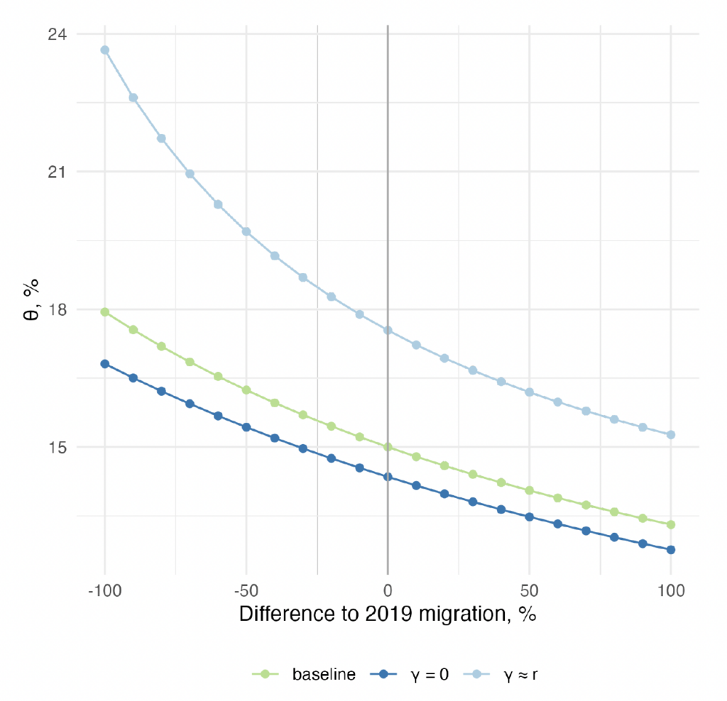
Note: The figure shows the $\theta_{\tau}$ value implied by different immigration scenarios. $\theta_{\tau}$ is computed according to Equation (8), under different values for the discount factor, $D$ .

1. High: Constant to the base year. This amounts to keeping constant the fertility of non-EU-born immigrants coming to the EA in 2019. This is an optimistic scenario as it seems more plausible that fertility will decline over time: the data on the fertility rates of developing countries show they have been decreasing in the last decades.

2. Low: Convergent to the natives’ value. The second alternative scenario is a rather pessimistic one. We set the fertility rate of non-EU immigrants to converge toward 1.6 children per woman, the same as nationals are expected to have by 2100.

We then recompute the rebalancing tax increase. Table E.2 shows this metric together with the $\theta_{\tau}^{AGK}$ and the $IBG$ . The differences are quite small across fertility scenarios. Even in the more extreme case, with immigrant fertility constant to the base year, $\theta_{\tau}$ only increases by 0.7 percentage points. This is due to an increase in the costs related to education that is not offset by a larger working-age population in the long run. On the other hand, a smaller fertility rate leads to a smaller rebalancing tax increase because of the same reasons. Nevertheless, the differences are not substantial for different non-EU-born fertility rates.

We then change the net migration scenario for the two additional fertility hypotheses. Figure E.2 plots the frontier between the level of migration and the imbalance factor for the different immigrants’ fertility hypotheses. The convex relationship between the two variables still holds, showing that the result is robust to this hypothesis as well.

Figure E.2. Frontier between the Level of Immigration and the Imbalance Factor for Different Immigrants’ Fertility Hypotheses

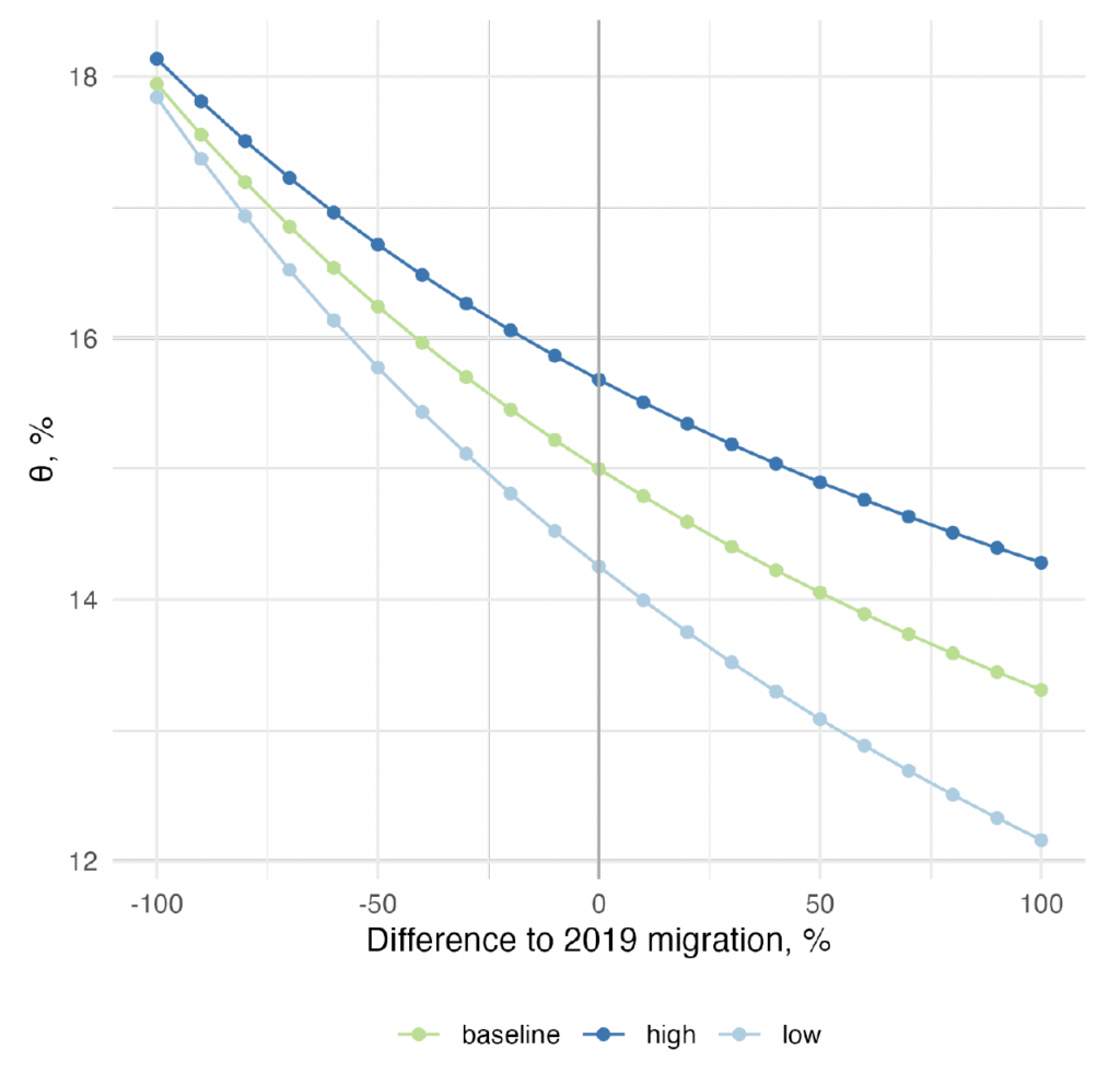
Note: Each line in the figure shows the relationship between $\theta_{\tau}$ and the immigration value in the EA, for different scenarios of non-EU-born fertility rates. $\theta_{\tau}$ is computed according to Equation (8).

F Additional Figures

Figure F.1. Primary Balance Decomposition by Demographic Characteristics for Different EA Countries

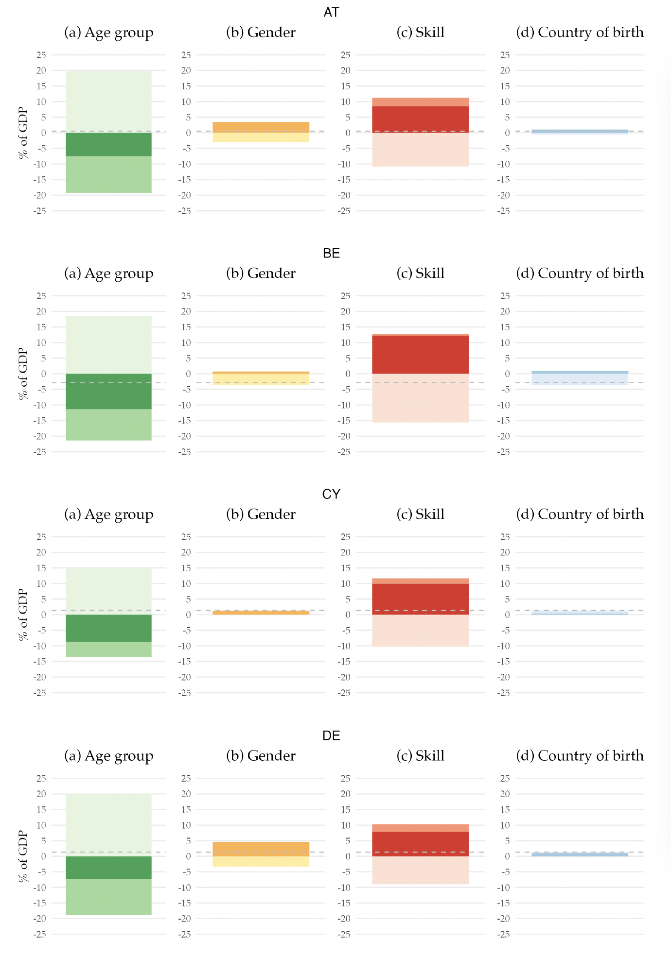
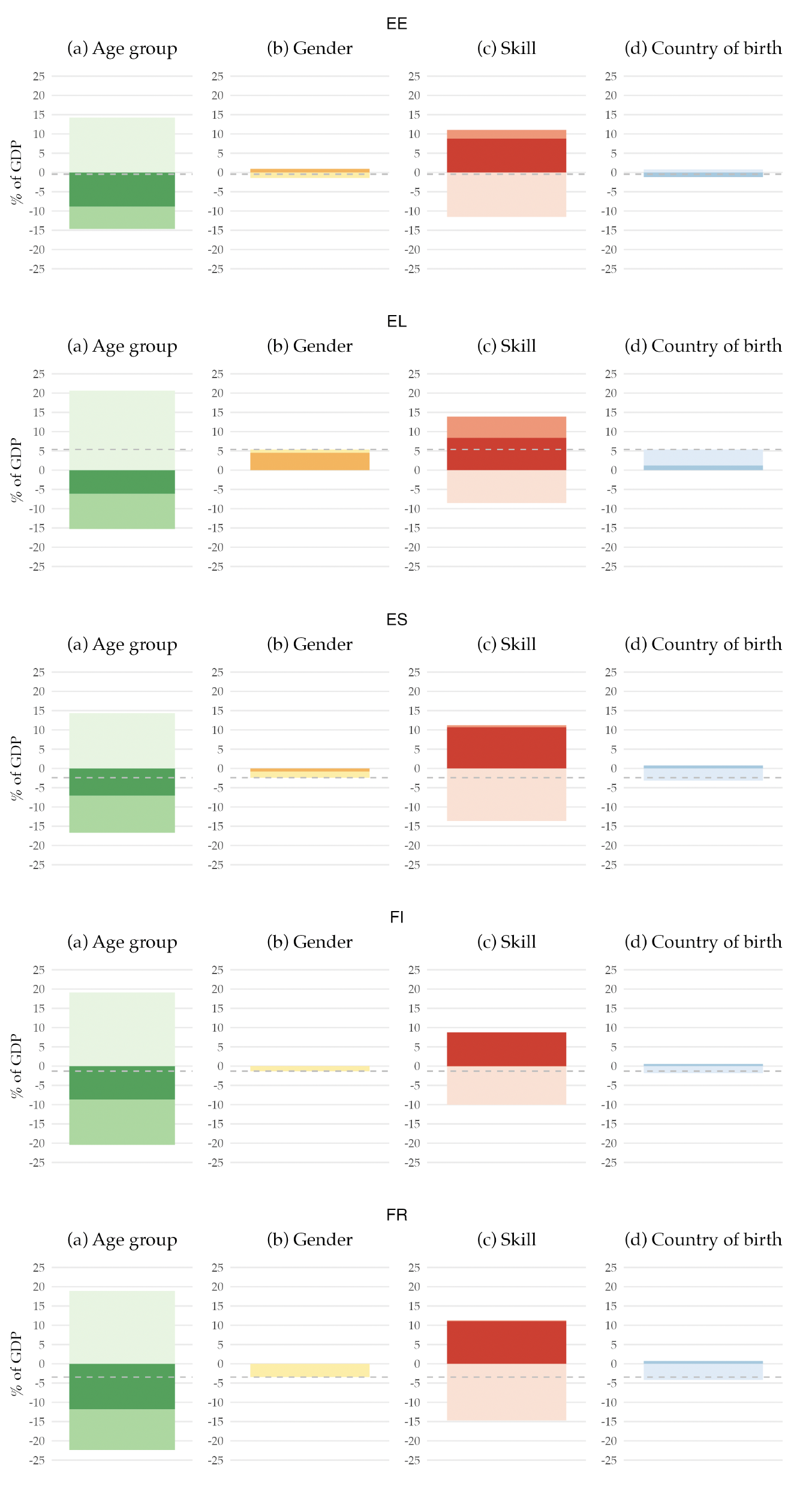
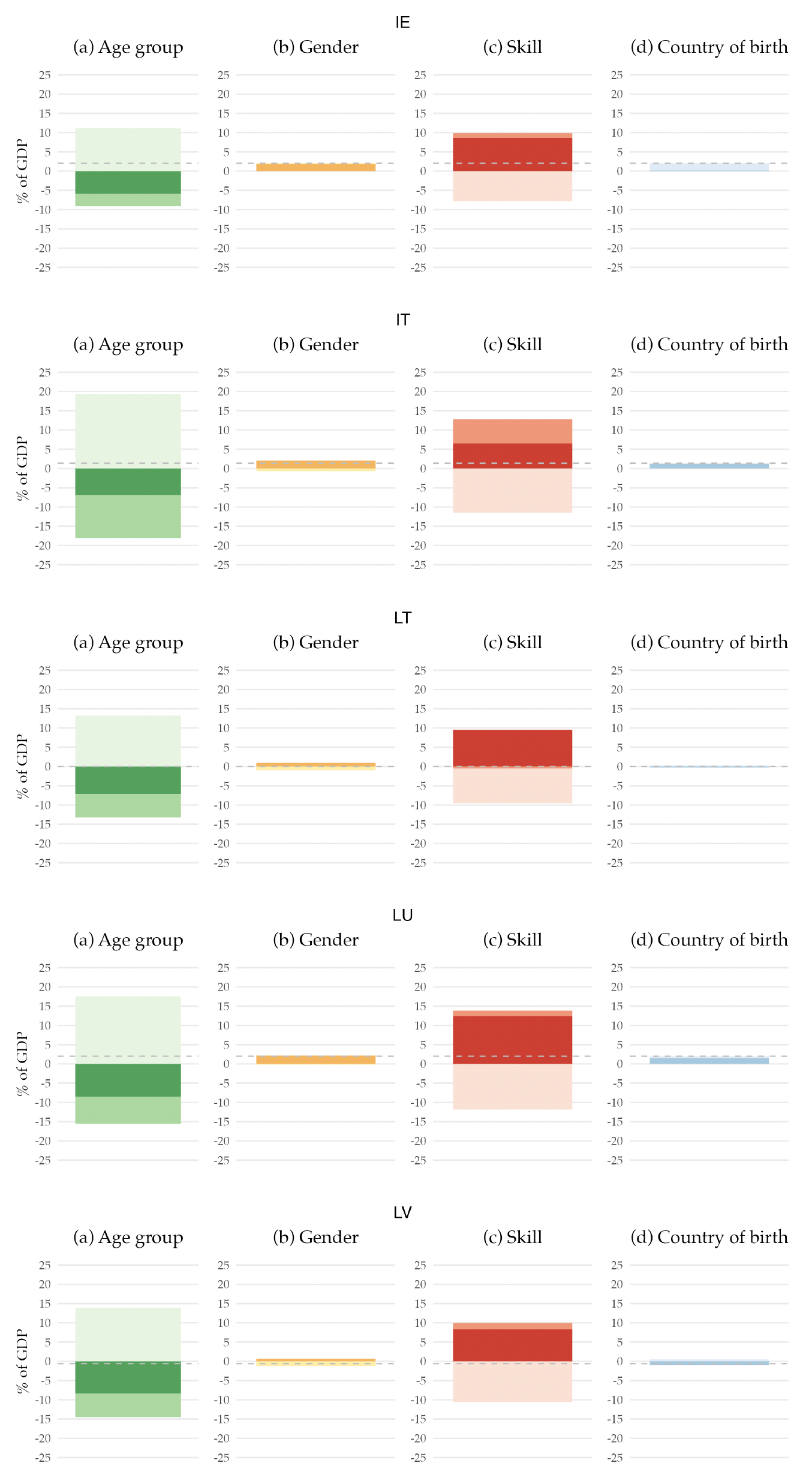
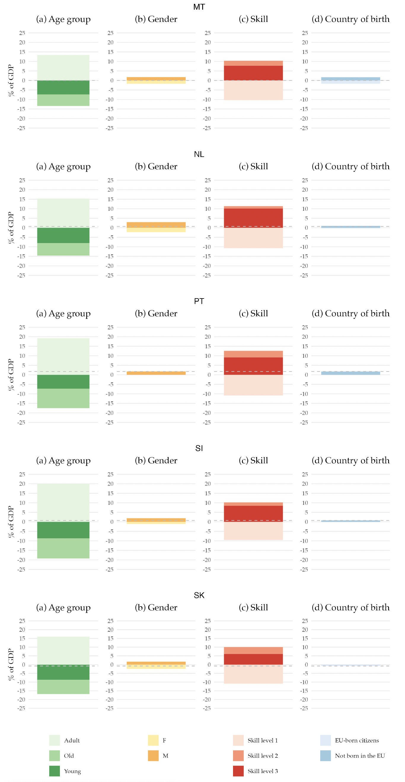
Note: The figure shows the primary balance decomposition by demographic characteristic for each country in the EA. It represents the sum of revenues, net of benefits, attributable to individuals with specific demographic characteristics, expressed as a percentage of the 2019 potential GDP. The dashed line indicates the value of the primary balance in 2019. All values are shown as a percentage of the potential GDP. The key for two-letter country codes is as follows: AT: Austria, BE: Belgium, CY: Cyprus, DE: Germany, EE: Estonia, EL: Greece, ES: Spain, FI: Finland, FR: France, IE: Ireland, IT: Italy, LT: Lithuania, LU: Luxembourg, LV: Latvia, MT: Malta, NL: the Netherlands, PT: Portugal, SI: Slovenia, and SK: Slovakia.

Figure F.2. Counterfactual Primary Balance Implied by the Population Projections Decomposed by Age Group and Country of Birth

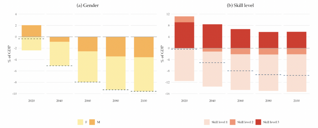
Note: The dashed lines in the figure represent the primary balance for selected years of the projection. The bars show the decomposition of the primary balance by skill level, where skill level 1 corresponds to the population who did not complete high school, skill level 2 corresponds to those who completed high school, and skill level 3 corresponds to those who completed college degree). All values are shown as a percentage of the potential GDP.

Figure F.3. Counterfactual Primary Balance Implied by the Population Projections for the Different EA Countries

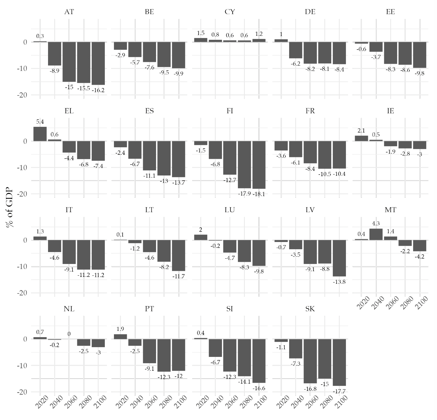
Note: The figure shows the primary balance implied by the population projections for selected years as a percentage of the potential GDP. The key for the two-letter country codes is as follows: AT: Austria, BE: Belgium, CY: Cyprus, DE: Germany, EE: Estonia, EL: Greece, ES: Spain, FI: Finland, FR: France, IE: Ireland, IT: Italy, LT: Lithuania, LU: Luxembourg, LV: Latvia, MT: Malta, NL: the Netherlands, PT: Portugal, SI: Slovenia, and SK: Slovakia.

References

Aging-Working-Group (2021). The 2021 aging report: Economic and budgetary projections for the EU member states (2019–2070). Technical report, Institutional Paper No. 148. Luxembourg: Publications Office of the European Union.

Auerbach, A. J., J. Gokhale, and L. J. Kotlikoff (1991). Generational accounts: A meaningful alternative to deficit accounting. Tax Policy and the Economy 5, 55–110.

Auerbach, A. J. and P. Oreopoulos (1999). Analyzing the fiscal impact of US immigration. American Economic Review 89 (2), 176–180.

Berti, K., A. Caretta, P. Eckefeldt, et al. (2019). The intergenerational dimension of fiscal sustainability. Technical report, Directorate General Economic and Financial Affairs (DG ECFIN), European Commission.

Bonin, H., C. Patxot, and G. Souto (2014). Cyclically neutral generational accounting. Fiscal Studies 35 (2), 117–137.

Bonin, H., B. Raffelhüschen, and J. Walliser (2000). Can immigration alleviate the demographic burden? FinanzArchiv 57 (1), 1.

Chojnicki, X. (2013). The fiscal impact of immigration in France: A generational accounting approach. World Economy 36 (8), 1065–1090.

Chojnicki, X. and P. E. Rabesandratana (2018). Aging, human capital, and productivity in France: A generational accounting perspective. Review of Income and Wealth 64 (4), 872–899.

Christl, M., A. Bélanger, A. Conte, J. Mazza, and E. Narazani (2022). Projecting the fiscal impact of immigration in the European Union. Fiscal Studies 43 (4), 365–385.

Coale, A. J. (1986). Demographic effects of below-replacement fertility and their social implications. Population and Development Review 12, 203–216.

Collado, M. D., I. Iturbe-Ormaetxe, and G. Valera (2004). Quantifying the impact of immigration on the Spanish welfare state. International Tax and Public Finance 11, 335–353.

D’Albis, H., E. Boubtane, and D. Coulibaly (2019). Immigration and public finances in OECD countries. Journal of Economic Dynamics and Control 99, 116–151.

Dustmann, C. and T. Frattini (2014). The fiscal and welfare effects of immigration. The Economic Journal 124 (580), 565–568.

Espenshade, T. J., L. F. Bouvier, and W. B. Arthur (1982). Immigration and the stable population model. Demography 19 (1), 125–133.

Eurostat (2020). Technical note: Summary methodology of the 2019-based population projections (EUROPOP2019).

Fehr, H., S. Jokisch, and L. J. Kotlikoff (2004). The role of immigration in dealing with the developed world’s demographic transition. FinanzArchiv 60 (3), 296.

Feist, K., B. Raffelhuschenm, and R. Vanne (1999). Finland: Macroeconomic turnabout and intergenerational redistribution. Generational Accounting in Europe 6.

Fiorio, C. V., T. Frattini, A. Riganti, and M. Christl (2023). Migration and public finances in the EU. International Tax and Public Finance, 1–50.

Franco, F., L. Teles Morais, T. Bernardino, and J. Jalles (2020). The implications of ageing for public finances in Portugal. Technical report, Gulbenkian Foundation.

Furlanetto, F. and Ø. Robstad (2019). Immigration and the macroeconomy: Some new empirical evidence. Review of Economic Dynamics 34, 1–19.

Girouard, N. and C. André (2006). Measuring cyclically-adjusted budget balances for OECD countries. Technical report, OECD.

Hansen, M. F., M. L. Schultz-Nielsen, and T. Tranæs (2017). The fiscal impact of immigration to welfare states of the Scandinavian type. Journal of Population Economics 30 (3), 925–952.

Lee, R. and T. Miller (2000). Immigration, social security, and broader fiscal impacts. American Economic Review 90 (2), 350–354.

Mayr, K. (2005). The fiscal impact of immigrants in Austria: A generational accounting analysis. Empirica 32 (2), 181–216.

Mitra, S. (1990). Immigration, below-replacement fertility, and long-term national population trends. Demography 27, 121–129.

Motiejunaite-Schulmeister, A., A. Sicurella, and P. Birch (2022). The structure of the European education systems, 2022/2023: Schematic diagrams. Technical report, ERIC.

Preston, I. (2014). The effect of immigration on public finances. Economic Journal 124 (580), F569–F592.

Price, R., T.-T. Dang, and J. Botev (2015). Adjusting fiscal balances for the business cycle: New tax and expenditure elasticity estimates for OECD countries. Technical report, OECD.

Rowthorn, R. (2008). The fiscal impact of immigration on the advanced economies. Oxford Review of Economic Policy 24 (3), 560–580.

Schmertmann, C. P. (1992). Immigrants’ ages and the structure of stationary populations with below-replacement fertility. Demography 29, 595–612.

Storesletten, K. (2000). Sustaining fiscal policy through immigration. Journal of Political Economy 108 (2), 300–323.

Storesletten, K. (2003). Fiscal implications of immigration: A net present value calculation. Scandinavian Journal of Economics 105 (3), 487–506.

Sutherland, H. and F. Figari (2013). EUROMOD: The European Union tax-benefit microsimulation model. International Journal of Microsimulation 6 (1), 4–26.

The Costs of Building Walls: Immigration and the Fiscal Burden of Aging in Europe

Executive Summary

Resources

Focuses

1 Introduction

2 Measuring Intertemporal Fiscal Imbalances

2.1 Mapping Budget Aggregates to Demographic Groups

2.2 Projecting toward the Future

2.3 Aggregation and Imbalance Metric

3 Data

3.1 Data Sources

3.2 Implementation

4 Demographic Profiles and Population Projections

4.1 Primary Balance Decomposition

4.2 Demographic Projections

5 Immigration and Public Finance Sustainability

5.1 The Fiscal Burden of Aging

5.2 The Nonlinear Effects of Immigration on Public Finances

5.3 Rebalancing Tax Increases at the Country Level

5.4 Robustness Exercises

6 Conclusion

Appendix

A Theoretical Background

A.1 Setup

A.2 Stable Population Results

A.3 Transitional Dynamics

B Additional Model Results

C Methodological Details

C.1 Cyclical-Neutral Fiscal Aggregates

C.2 Other Metrics for Comparison

C.3 Estimation of the Age, Gender, Skill, and Country of Birth Profiles

C.4 Building Population Projections

D Additional Data Source Details

D.1 Microdata Sources

D.2 Macrodata Sources

E Robustness Tests

E.1 Macroeconomic Hypothesis

E.2 Immigrant Fertility

F Additional Figures

References

Executive Summary

Resources

Related Publications

Related News

Related Blogs

Focuses

1 Introduction

2 Measuring Intertemporal Fiscal Imbalances

2.1 Mapping Budget Aggregates to Demographic Groups

2.2 Projecting toward the Future

2.3 Aggregation and Imbalance Metric

3 Data

3.1 Data Sources

3.2 Implementation

4 Demographic Profiles and Population Projections

4.1 Primary Balance Decomposition

4.2 Demographic Projections

5 Immigration and Public Finance Sustainability

5.1 The Fiscal Burden of Aging

5.2 The Nonlinear Effects of Immigration on Public Finances

5.3 Rebalancing Tax Increases at the Country Level

5.4 Robustness Exercises

6 Conclusion

Appendix

A Theoretical Background

A.1 Setup

A.2 Stable Population Results

A.3 Transitional Dynamics

B Additional Model Results

C Methodological Details

C.1 Cyclical-Neutral Fiscal Aggregates

C.2 Other Metrics for Comparison

C.3 Estimation of the Age, Gender, Skill, and Country of Birth Profiles

C.4 Building Population Projections

D Additional Data Source Details

D.1 Microdata Sources

D.2 Macrodata Sources

E Robustness Tests

E.1 Macroeconomic Hypothesis

E.2 Immigrant Fertility

F Additional Figures

References