Skilled Immigration Frictions as a Barrier for Young Firms

Mandelman, Federico; Mehra, Mishita; Shen, Hewei

1 Introduction

Skilled immigration policies in the United States, notably those involving the H-1B visa program, impose well-known frictions on firms. This program, the largest channel for hiring temporary foreign workers with at least a bachelor’s degree, involves several implicit and explicit costs. Additionally, there is a fixed aggregate quota of H-1B visas for private firms each fiscal year. Since 2004, when this quota is reached, visas are allotted through a random lottery.¹

The potentially larger impacts of these policy-imposed frictions on young, emerging firms in technology-intensive sectors have often been overlooked. Firms in multiple surveys have mentioned that H-1B policy restrictions are particularly onerous for emerging firms. GAO (2011) reports that in years when visas were limited by the cap, most large firms found alternative (and costly) ways to hire their preferred candidates. For instance, large multinational firms can hire skilled foreign workers in offshore affiliates (Glennon, 2020).² In contrast, small firms, as mentioned in the same survey (GAO, 2011), are more likely to fill their positions with different candidates. This often leads to delays and economic losses, particularly for firms in rapidly changing technology fields. Entrepreneurs interviewed also mentioned that H-1B regulations prevent many emerging technology companies from using the H-1B program to source the talent they need, constraining their ability to grow and innovate in the United States. This issue arises partly because small, emerging companies in high-tech sectors often require extremely specialized skills, and these firms cannot always find a suitable “second-choice” employee in the US labor market.³

Within this context, we study the impacts of current US skilled immigration policy frictions on young technology-intensive firms. We first evaluate the impact of H-1B visa lottery win rates (similar to Dimmock et al., 2021 and recently Brinatti et al., 2023) in fiscal years 2014 and 2015 on firm survival in subsequent years. To do this, we combine proprietary establishment-level data from the National Establishment Time Series (NETS) with firm-level data on Labor Condition Applications (LCAs) and H-1B petitions. This approach allows us to investigate how the random allocation of H-1B visas constrains firm operations. Our findings confirm that lower H-1B visa win rates significantly impact the survival of young firms (aged 0–5) in technology-intensive sectors, whereas this impact is not significant for older firms. We then include key skilled immigration policy frictions that mimic the H-1B policy and skilled foreign worker accumulation into a general equilibrium model based on Hopenhayn & Rogerson (1993). We find that eliminating major immigration policy frictions would increase average productivity in the high-tech sector. The main mechanism is through the increased entry and survival of younger firms, which leads to a greater exit of older, less productive firms.

There are several reasons why focusing on high-tech sectors is important within this framework. First, these sectors are directly linked to H-1B visa demand, with firms in high-tech sectors constituting 65 percent of the demand for skilled foreign workers.⁴ Second, the share of young high-tech firms has declined since the early 2000s, even when compared to the overall percentage of young firms across all sectors (Figure 1).⁵ Haltiwanger et al. (2014) emphasize the important role of young (aged 0–5), high-tech businesses in job creation and productivity and document the secular decline in the number of young high-tech firms after 2002.⁶ Importantly, this decline cannot be explained by business consolidation spurred by an increase in market power in recent decades. Evidence of this trend can be seen in the increase in the share of the smallest firms (with 1–19 employees) among the oldest age cohorts (aged 11 and older) in high-tech firms, as shown in Figure 2. In contrast, the non-high-tech sector has witnessed a clear declining trend in the share of the smallest firms among the oldest firms.

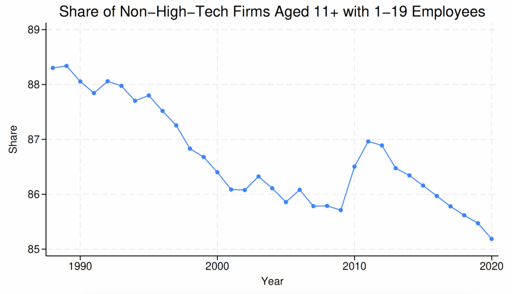
Note that the aging of the high-tech sector firms and the increase in the share of smaller firms within older firms coincided with a period of more restrictive skilled immigration policy. As seen in Figure 3, the H-1B cap fell from 195,000 in 2003 to 85,000 in 2005 and has remained constant since then. At the same time, this period witnessed an increasing demand for skilled foreign workers, as measured by LCAs. Given the high fraction of demand for skilled foreign workers in high-tech sectors and the trends observed in high-tech sectors since the early 2000s, it is important to analyze the impact of skilled immigration policy restrictions on young high-tech firms. This is particularly relevant given the recent push to bring high-tech production back to the United States (e.g., the Bipartisan Innovation Act).

While there has been extensive literature on the impacts of US skilled immigration policy, to the best of our knowledge, no study has specifically emphasized the effects of current policy frictions on younger firms nor has studied the direct effect on firm dynamics and general equilibrium impacts in the macroeconomy. This paper aims to fill this gap by studying both the direct impacts of frictions using firm-level data and general equilibrium impacts by age cohorts, using a quantitative general equilibrium model disciplined by data.

Our model is based on Hopenhayn & Rogerson (1993) with foreign labor accumulation and endogenous firm entry and exit. Firms in the technology-intensive sector face heterogeneous idiosyncratic productivity shocks. While they can hire skilled domestic workers, they may also want to hire skilled foreign workers, for two reasons. First, foreign and domestic workers are imperfect substitutes, and access to foreign workers reduces the per-effective worker wage cost. Second, foreign workers are more productive than domestic workers for the same wages.

Figure 1. Share of High-Tech Young Firms in All Young Firms

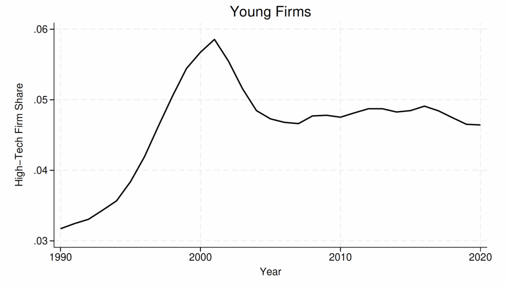
Notes: The figure is compiled using the US Census Bureau’s Business Dynamics Statistics (BDS). High tech firms are computed using four-digit NAICS codes and the BLS classification (Heckler, 2005). Young firms are defined as those with ages between 0 and 5.

Similar to the actual H-1B visa policy for skilled immigrant workers, our model features three immigration policy-imposed frictions for firms wanting to hire skilled foreign workers. First, there is a one-time sunk cost, which represents the cost of learning skilled immigration regulations and building connections with law firms that can help with the legal process of hiring foreign workers. Second, firms that have paid the sunk cost may face a negative idiosyncratic hiring shock, preventing them from hiring additional skilled foreign workers. This captures frictions similar to the H-1B lottery such that some firms cannot hire foreign workers even if they are willing to pay costs. Third, there is a per-worker hiring fee paid by firms that have overcome the first two frictions and end up hiring skilled foreign workers in a given period. This mimics the H-1B petition fee required for each worker.⁷

The model is calibrated to match the US economy between 2005 and 2020, using data from the Business Dynamics Statistics (BDS), the Current Population Survey (CPS), and the US Citizenship and Immigration Services (USCIS). The distribution of firms in the model by age cohorts is consistent with the corresponding distribution in the data. Using value function iteration for solving the decentralized equilibrium, our model demonstrates how changes in immigration policies can influence firm dynamics consistent with the data trends.

Figure 2. Share of Smallest Firms in Oldest Age Cohorts

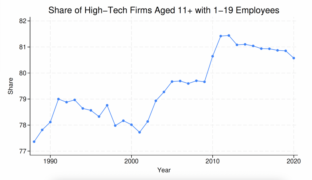
Notes: The figure is compiled using the US Census Bureau’s BDS. The upper (lower) panel corresponds to the high-tech sector (non-high-tech sector). High-tech firms are computed using four-digit NAICS codes and the BLS classification (Heckler, 2005).

Our counterfactual policy exercises show that easing immigration policy frictions has the following effects. All firms will have a higher chance of increasing their hiring of foreign workers, which is beneficial due to the imperfect substitutability between domestic and foreign workers and additional productivity gains from hiring foreign workers. Therefore, there is a higher chance that new entrants can hire foreign workers immediately, which increases the chance of survival, consistent with our empirical results. In a counterfactual environment with no skilled immigration policy frictions, there is a higher mass of entrants, a lower exit rate of younger firms, a larger foreign labor stock, and a higher aggregate skilled-intensive output produced but a lower average production per firm. Moreover, a higher mass of firms in the economy feeds into a higher cost of production and lowers the profits of incumbent firms. Therefore, older, less productive incumbents are pushed out of the market, increasing the average exit rate of older firms and the increasing productivity of all firms.

Figure 3. LCAs versus H-1B Cap

We also evaluate the impact of the change in the extensive margin of firms on skilled domestic workers. More than one-third of domestic workers are absorbed by the additional firms that exist due to lower immigration frictions. These additional firms contribute toward a 17.9 percent change in the welfare of skilled domestic workers by the extensive margin relative to the case with immigration frictions.

Finally, we find that the results of the general equilibrium model are consistent with trends in the data after immigration policy frictions were increased in 2004 (via the H-1B cap reduction). The period with higher immigration policy frictions since 2005 witnessed a lower average exit rate of older firms, an increase in the average share of older firms, and an increase in the share of the smallest (less productive) firms within the oldest firms in the high-tech sectors. These trends are consistent with the predicted impacts of our model after an increase in immigration policy frictions.

Empirical literature provides limited evidence on how the H-1B policy impacts the outcomes of new firms. Dimmock et al. (2021) show that start-ups with higher win rates of H-1B visas in the 2008–2009 fiscal years were more likely to access credit, implement successful initial public offerings, and file patents. In contrast, we focus on young firms in high-tech sectors and general equilibrium impacts in addition to firm-level impacts.

Empirical evidence also exists on the impact of immigration worker inflows on business growth. Mahajan (2022) shows that inflows of immigrant workers lead to an increased exit of establishments in smaller (less productive) firms. This mechanism is consistent with our model’s main mechanism—higher immigrant inflows cause new firms to enter the market, leading to the exit of older, less productive firms. Brinatti et al. (2023) find that skilled-intensive firms expand the most after winning the H-1B lottery. Orrenius et al. (2020) use the NETS database (from 1997 to 2013) and CPS data and find that immigration (particularly of less-educated individuals) boosts business survival and raises employment by reducing job destruction. Olney (2013) uses data from the CPS and the Statistics of US Businesses and finds that an increase in unskilled immigrants raised the number of establishments between 1998 and 2008.

This paper is also related to the empirical literature on the impact of skilled immigration in the United States (via the H-1B policy) on firms, cities, productivity, and hiring practices (S. P. Kerr et al., 2014; W. R. Kerr & Lincoln, 2010; S. P. Kerr et al., 2013; Doran et al., 2016; Peri et al., 2014; Peri et al., 2015a; Ottaviano et al., 2018; Glennon, 2020; Raux, 2023) and papers studying the general equilibrium impacts of US skilled immigration policies (Bound et al., 2015; Waugh, 2018; Bound et al., 2017; Mehra & Shen, 2022).⁸ To the best of our knowledge, no study has focused on the general equilibrium misallocation impacts of skilled immigration policies on emerging firms and the aggregate implications. Stochastic heterogeneous firm productivity with foreign worker accumulation allows us to study the distortionary impacts of immigration policy on the entry, survival, and growth of firms in skilled-intensive sectors. The model is related to the literature studying the persistent role of entry and exit dynamics in response to aggregate shocks (e.g., Hopenhayn 1992 and Clementi & Palazzo 2016). Using BDS data, Sedláček (2020) also finds that changes in firm entry impact the economy both directly and indirectly as start-up cohorts age. While these papers focus on the aggregate impacts of productivity shocks and recessions, ours highlights that distortions imposed by skilled immigration policies can have persistent aggregate impacts.

The paper also relates to the literature studying policy distortions and the aggregate impacts of allocative efficiency across heterogeneous firms. Hopenhayn & Rogerson (1993) extend the Hopenhayn (1992) model and evaluate the equilibrium effects of tax policies on the labor market. They find that a tax on job destruction at the firm level has a sizable negative impact on total employment, average productivity, and welfare. Gabler & Poschke (2013) build a model with endogenous risky experimentation decisions chosen by firms and study the distortionary effects of different tax policies on aggregate productivity, firm dynamics, and welfare. Bento & Restuccia (2017) consider a model of heterogeneous production units with endogenous entry and productivity investment to assess the quantitative impact of policy distortions. Ranasinghe (2014) examines the dynamic effects of distortions when they affect both the allocation of resources and firm-level incentives to improve productivity. Mukoyama & Osotimehin (2019) study how factors hindering the reallocation of inputs across firms influence aggregate productivity growth. They extend the model of Hopenhayn & Rogerson (1993) model to allow endogenous innovation, and evaluate the effects of firing taxes on reallocation, innovation, and productivity growth. Last, Sedláček & Sterk (2019) use a quantitative heterogeneous firm model and investigate the long-run effect of the 2017 tax reforms on firm dynamics. They find that the reform can substantially increase business dynamism, potentially offsetting the large decline in the US start-up rate observed over recent decades.

3 Empirical Evidence

To motivate our focus on young firms in technology-intensive sectors, we first use firm-level data to confirm that skilled immigration policy frictions (via the H-1B visa policy) impact young firms in technology-intensive sectors. We focus on evaluating the impact of H-1B lottery win rates on firm survival in the years following the lottery.

Our identification strategy exploits the exogenous variation in firms’ H-1B visa lottery outcomes to identify whether access to skilled foreign workers constrains a firm’s ability to continue operations. H-1B visas were allocated through a lottery in fiscal years 2008 and 2009 and in each fiscal year from 2014 onward.⁹ We use the lottery years from fiscal years 2014 and 2015 and compute an average H-1B lottery win-rate measure in these years. By focusing on these particular fiscal years, we avoid the impacts of the earlier recession years. The H-1B visa win rate for each firm is measured as the ratio of approved petitions to the demand for visas,¹⁰ therefore indicating firm-level hiring constraints or firm-level frictions due to H-1B immigration policies. To compute win rates, we combine data on approved H-1B visas (from the USCIS H-1B Employer Data Hub) with the indicated demand for visas for fiscal years 2014 and 2015. For the measure of demand, we use LCAs filed between February and April of each calendar year with a start date five to six months away, similar to the literature.¹¹ Our H-1B win-rate measure is similar to Dimmock et al. (2021) and, recently, Brinatti et al. (2023).¹²

We then match the firm-level win rates to firm outcomes using the NETS database by probabilistically matching firms by names and location (city) to create a panel data set from 2011 to 2020. To measure firm-level variables like survival, employment, and age, we collapse across all establishments at the HQ company level to obtain firm-level variables. The NETS database includes private for-profit and nonprofit organizations and public sector organizations. The data include four-digit NAICS industry codes that help infer technology levels of firms using Heckler (2005) classifications. The annual data depict business indicators in January of a given year. We only keep firms in our sample that have applied for skilled foreign workers in fiscal years 2014 and 2015.

For our main dependent variable, we define $\text { Survive }_{i,t} = 1$ if a firm that was active in the calendar year 2014 remains active in postlottery calendar year $t$ , where $t$ = 2015, 2016, 2017, 2018, and 2019. Note that H-1B lottery outcomes for fiscal years 2014 and 2015 were announced in April 2013 and April 2014, with an employment start date in October 2013 and October 2014, respectively. Therefore, the lottery outcomes in fiscal years 2014 and 2015 correspond to outcomes in calendar years 2013 and 2014, respectively. We define $\text { Survive }_{i,t} = 0$ if a firm both became inactive in our postlottery calendar years and did not undergo a merger/acquisition.¹³ The latter ensures that our firm survival variable does not mistakenly count a merger as a closure. While mergers/acquisitions can be a positive outcome for young firms in technology sectors, we exclude such outcomes given the lack of detailed data in NETS on the values of the mergers/acquisitions. Our final sample includes 15,200 unique firms in the LCA database matched with the NETS database. To the best of our knowledge, no previous study has matched H-1B data to the NETS database to evaluate the impacts of the H-1B lottery.¹⁴

Table 1 displays the summary statistics of key variables used in our main analysis. The average win rate for each application in our full sample is 39 percent. This rate is very close to the actual average approval rate for H-1B initial employment reported by the USCIS in fiscal years 2014 and 2015 (40 percent).¹⁵

Figure 4 first plots the average fraction of firms that survived during calendar years 2015–2019 in the raw data. On average, a larger fraction of firms with a win rate of 1 (in fiscal years 2014 and 2015) survived in the postlottery years compared to firms with a win rate of 0. This difference is noticeable for high-tech firms and young high-tech firms separately but less for older high-tech firms.

Figure 4. Raw Data: Average Proportion of Surviving Firms

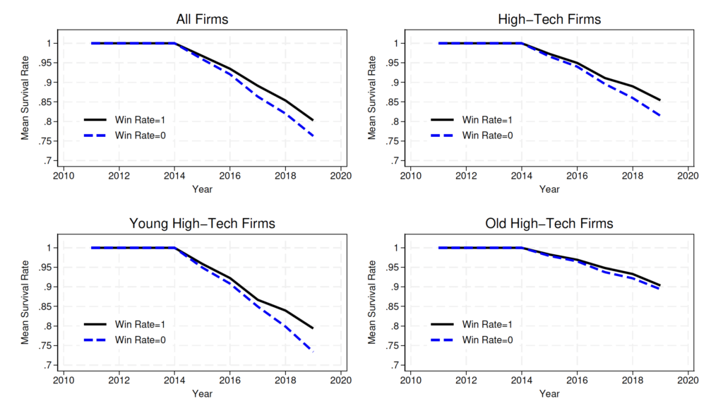
Notes: Win Rate = 1 includes firms that received 100 percent of their requested skilled foreign workers during fiscal years 2014 and 2015. Win Rate = 0 includes firms that received 0 percent of their skilled foreign workers. We exclude mergers/acquisitions.

To test these impacts, we use a difference-in-difference panel regression similar to Brinatti et al. (2023) with firm, year, and industry-by-year fixed effects, to study the impact of a firm’s win rate on its survival status in the postlottery calendar years. The results in Table 2 establish that higher average H-1B lottery win rates positively and significantly impact the survival of all firms. For the full sample (column 1), firms that won the lottery for 100 percent of the workers they applied for increased their average survival by 2.6 percentage points, compared to those that had all their H1B applications rejected.¹⁶ When comparing the results across different subsamples of firms, a 100 percent win for a young high-tech firm means, on average, a higher survival by 3.5 percentage points (column 3) compared to a win rate of 0. In contrast, the impact of the win rate on older firms (aged 6+) is not significant (column 4).

In summary, the results confirm our intuition that young firms in technology-intensive sectors are more likely to face constraints of immigration policy frictions relative to older firms. Next, we incorporate a more general set of immigration policy frictions that are similar to US policies into a general equilibrium model. This approach allows us to study the impacts of these frictions on high-technology firms by age and on average productivity.

4 Model

In this section, we incorporate international skilled immigration policy that mimics the H-1B policy into a heterogeneous firm model à la Hopenhayn (1992) and Hopenhayn & Rogerson (1993). Time is discrete, and the economy lasts for an infinite number of periods ( $t$ = 0, 1, 2 . . .).

The model features a two-sector economy that is populated with skilled (domestic and foreign) and unskilled households. Sector 1 (the skilled sector) consists of an endogenous measure of firms. In the context of this paper, which focuses on the influence of immigration policies on the entry and dynamics of high-tech companies, this sector is interpreted as the high-tech industry, and it hires skilled workers. Sector 2 (the unskilled sector) firms are interpreted as other firms that hire relatively lower-skilled (unskilled) workers. Sector 1 firms produce output using domestic and skilled foreign labor and are subject to idiosyncratic productivity and foreign worker hiring shocks. In addition, the measure of sector 1 firms is endogenous as firms make optimal entry and exit decisions. Sector 2 consists of a representative firm that produces output using unskilled labor. The consumption bundle of households includes outputs from both the skilled and unskilled sectors, and therefore the model features complementarities of skilled and unskilled workers via the consumption bundle.

In each period, only a subset of sector 1 firms hire skilled foreign labor. Skilled immigration policies in the United States impose regulatory frictions and lawyer fees that are borne by the firm. To capture this, we assume that sector 1 firms must pay a one-time sunk cost if they want to be able to hire skilled foreign labor. This cost captures the time and money spent in gaining knowledge of immigration policies, building lawyer relationships, etc. Since not all firms pay this sunk cost, a subset of sector 1 firms produce output using only skilled domestic workers.

Each period, all sector 1 firms hire skilled domestic workers. While sector 1 firms that have already incurred the sunk hiring cost want to hire foreign workers, additional immigration policy frictions prevent them from doing so each period. We assume that these firms face an idiosyncratic shock each period that prevents them from hiring additional foreign workers in that period. If an unfavorable hiring shock hits a firm, it can hire, at most, the foreign workers carried from the last period, less the foreign workers exogenously leaving the country. In contrast, if a favorable shock is realized, the firm can increase the number of foreign workers hired by paying an adjustment cost, that is, a hiring cost for each foreign worker. The idiosyncratic hiring shock is a simplistic way to capture that sometimes firms may not be able to acquire the foreign workers they desire due to unfavorable results from the H-1B lottery.

In addition, similar to Mehra & Shen (2022), we assume that skilled foreign workers are an imperfect substitute for skilled domestic labor, as they both are assumed to earn the same wages. This assumption is consistent with the H-1B hiring regulations: when sponsoring a worker for an H-1B visa, a firm must attest that they will pay the worker the prevailing compensation for that occupation. If it decides not to hire any new foreign workers, it may produce with only skilled domestic workers. Once foreign workers are hired, they will stay with the firm until an exogenous separation shock is realized or when the firm decides to fire them.

We focus on the domestic economy and do not model the rest of the world explicitly. Instead, we assume there is a foreign country that has a large elastic supply of skilled workers who domestic firms can hire. Last, all prices are expressed in units of the final consumption basket.

4.1 Firms

In this section, we describe the challenges faced by firms in our model, beginning with skilled-intensive firms due to the key role their dynamics play in our framework. We then discuss the issues pertaining to unskilled-intensive firms. Since we write the firms’ problems recursively, we suppress the time notation when describing them.

4.1.1 Skilled-Intensive Sector (Sector 1)

The skilled-intensive firms in our model represent the high-tech firms we focus on in this paper, and therefore we explicitly model their entry and exit decisions. The issues of these firms are similar to those of the firms described in Sedláček & Sterk (2019). They are owned by skilled domestic households and produce a homogeneous good, maximizing the present discounted value of profits. They use a decreasing returns-to-scale production function $y=f\left(z, l^s\right)$ , where $y$ is the output and $z$ is the firm-specific productivity and follows a Markov process. $l^s$ is the composite skilled labor, which depends on both the domestic $(l^d)$ and foreign $(l^f)$ skilled labor employed if the firm has paid the one-time sunk cost and hires a foreign worker. If the firm does not hire any foreign workers, it only employs skilled domestic workers to produce. We denote the firms that only hire skilled domestic workers as type- $d$ firms and those that hire both skilled domestic and foreign workers as type- $f$ firms.

Hired foreign workers leave their jobs at an exogenous rate of $\delta \in(0,1)$ , and new hiring is denoted as $n=l^f-(1-\delta) l_{-1}^f$ , where $l_{-1}^f$ is the stock of foreign workers from the last period. New foreign workers start producing in the same period of hire. Because firms must pay the filing cost of H-1B visas, they face a hiring cost when hiring foreign workers, denoted as $\psi\left(l^f, l_{-1}^f\right)$ . At the beginning of a period, a type- $d$ firm can pay a sunk cost $c_s$ to become a type- $f$ firm and start the hiring process in the same period. Last, both types of firms also face an operation cost of $c_f$ . The hiring cost, sunk cost, and operation cost are all denominated in units of the skilled-intensive sector good.

Incumbent firms. At the beginning of each period, an incumbent firm, whether type $d$ or type $f$ , decides on whether to exit the market or continue operations. The decision is based on the firm-specific stock of foreign workers, $l_{-1}^f$ (0 for type $d$ ), and productivity from the last period, $z_{-1}$ . If the firm decides to exit the market, it receives an outside value of 0 and fires all remaining foreign workers. If the firm decides to continue operations, a type- $d$ firm may pay the sunk cost to become a type- $f$ firm in the same period.

Next, both types of firms learn their new productivity, which evolves based on a log AR(1) process

(1) $\begin{equation*}\log (z)=\left(1-\rho_z\right) \mu_z+\rho_z \log \left(z_{-1}\right)+\varepsilon,\end{equation*}$

where $\varepsilon$ is a firm-specific productivity shock. After learning about its productivity, a type- $f$ firm faces an idiosyncratic hiring shock, which determines if it can hire additional foreign workers in the same period. As mentioned earlier, we assume the skilled foreign worker earns the same wage as the skilled domestic worker.

Both types of firms then make hiring decisions. Type- $d$ firms only hire domestic workers, while type- (f\) firms can hire foreign workers by paying hiring costs $\left(\psi\left(l^f, l_{-1}^f\right)\right)$ . If a type- $f$ firm receives an unfavorable hiring shock, it can produce with at most $(1-\delta) l_{-1}^f$ foreign workers and as many domestic workers as it wants. With a favorable hiring shock, a type- $f$ firm can hire as many domestic and foreign workers as it wants. All firms pay the operation cost, $c_f$ , and produce the sector 1 good. Each firm is also small, so it takes the prices and wages as given when deciding. Denote $V^{I D}\left(z_{-1}\right)$ and $V^{I F}\left(l_{-1}^f, z_{-1}\right)$ as the beginning-of-period values for the incumbent type- $d$ and type- $f$ firms. The value of a type- $d$ firm that decides to stay but does not become a type- $f$ firm is given by

(2) $\begin{equation*}W^d(z)=\max _{l^d}\left{\left[p_1 f\left(z, l^s\right)-p_1 c_f-w_s l^d\right]+\beta V^{I D}(z)\right}\end{equation*}$

(3) $\begin{equation*}\text { s.t. } l^s=l^d \text {. }\end{equation*}$

The value of a type- $f$ firm that decides to stay but faces an unfavorable hiring shock is given by

(4) $\begin{equation*}W^{f u}\left(l_{-1}^f, z\right)=\max {n, l^f, l^d}\left{\left[p_1 f\left(z, l^s\right)-p_1\left(\psi\left(l^f, l{-1}^f\right)+c_f\right)-w_s\left(l^d+l^f\right)\right]+\beta V^{I F}\left(l^f, z\right)\right}\end{equation*}$

(5) $\begin{equation*}\text { s.t. } l^f=n+(1-\delta) l_{-1}^f \text {, }\end{equation*}$

(6) $\begin{equation*}n \leq 0\end{equation*}$

(7) $\begin{equation*}l^s=\left[\left(l^d\right)^\gamma+\left(a l^f\right)^\gamma\right]^{\frac{1}{\gamma}},\end{equation*}$

where $\psi\left(l^f, l_{-1}^f\right)$ is the hiring cost of an additional foreign worker, with $\psi\left(l^f, l_{-1}^f\right)>0$ if $l^f>(1-\delta) l_{-1}^f$ and 0 otherwise. $p_1$ is the price of the skilled-intensive sector good. $l^s$ is the aggregate skilled labor hired by the firm, and $1 /(1-\gamma)$ is the elasticity of substitution between skilled domestic and foreign workers. $\beta \in(0,1)$ is the subjective discount factor for the skilled domestic households, who are the owners of the skilled-intensive sector firms.¹⁷

$a>1$ represents the additional productivity that foreign workers bring to production, and this assumption generates additional incentives for hiring skilled immigrant workers. By law, firms must pay a cost for hiring skilled immigrant workers and pay the same prevailing skilled wages to workers as denoted by $w_s$ . These conditions would generate limited incentives for hiring skilled foreign workers, which is inconsistent with the data on the number of applications submitted for skilled immigrant workers that indicate a huge demand for such workers. Therefore, we assume a positive productivity gain from hiring skilled foreign workers, which is also consistent with empirical evidence in Peri et al. (2015b).

A type- $f$ firm that decides to stay but receives a favorable hiring shock can hire additional skilled foreign workers and face the following issue:

(8) $\begin{equation*}W^{f f}\left(l_{-1}^f, z\right)=\max {n, l^f, l^d}\left{\left[p_1 f\left(z, l^s\right)-p_1\left(\psi\left(l^f, l{-1}^f\right)+c_f\right)-w_s\left(l^d+l^f\right)\right]+\beta V^{I F}\left(l^f, z\right)\right}\end{equation*}$

(9) $\begin{equation*}\text { s.t. } l^f=n+(1-\delta) l_{-1}^f \text {, }\end{equation*}$

(10) $\begin{equation*}l^s=\left[\left(l^d\right)^\gamma+\left(a l^f\right)^\gamma\right]^{\frac{1}{\gamma}} .\end{equation*}$

At the beginning of the period, firms decide whether to exit the market or continue operations. Specifically, firms that have foreign workers at the beginning of the period solve

(11) $\begin{equation*}V^{I F}\left(l_{-1}^f, z_{-1}\right)=\max \left{W^F\left(l_{-1}^f, z_{-1}\right), 0\right},\end{equation*}$

where $W^F\left(l_{-1}^f, z_{-1}\right)=\mathbb{E}{z \mid z{-1}}\left[q \times W^{f f}\left(l_{-1}^f, z\right)+(1-q) \times W^{f u}\left(l_{-1}^f, z\right)\right]$ and $q$ is the probability that an incumbent type- $f$ firm receives a favorable hiring shock. We normalize the value of exiting the market to 0.

For an incumbent type- $d$ firm, it can choose to either exit the market, stay in the market and continue to be type $d$ , or stay in the market and pay a sunk cost $c_s$ to become type $f$ . Specifically, its value function is

(12) $\begin{equation*}V^{I D}\left(z_{-1}\right)=\max \left{\mathbb{E}{z \mid z{-1}} W^d(z), W^F\left(0, z_{-1}\right)-p_1 c_s, 0\right} .\end{equation*}$

Since the value function $V^{I F}\left(l_{-1}^f, z_{-1}\right)$ is increasing in the productivity $z_{-1}$ , there exists a productivity cutoff point $z^{I *}\left(l_{-1}^f\right)$ for each level of $l_{-1}^f$ such that firms with a productivity $z_{-1} \geq(<) z_f^{I *}\left(l_{-1}^f\right)$ will choose to continue operations (exit the market). A similar argument applies to type- $d$ firms.

New entries. There is free entry of firms. After paying a cost of $c_e$ , an entrant may enter the market and draw a $z_{−1}$ from a distribution.¹⁸ Then, the new entrant, just like incumbents, can choose to immediately exit or continue operations. Similar to Hopenhayn & Rogerson (1993) and Sedláček & Sterk (2019), we assume the entrants start as type- $d$ firms.

Denote $V^e\left(z_{-1}\right)$ as the value of the new entry with a productivity $z_{−1}$ drawn. Free entry implies that firms keep entering the market until $\mathbb{E}<em>e V^e\left(z</em>{-1}\right)=p_1 c_e$ . The endogenous entry decisions allow us to quantitatively evaluate the effects of immigration policies on new firm formation and compare them with the data.

Since the entering firms face the same problem as the incumbent type- $d$ firms, the continuing entering firm’s problem is given by

(13) $\begin{equation*}W^e(z)=W^d(z) .\end{equation*}$

Then, the value of the newly entered firm $V^e(z)$ is defined as

(14) $\begin{equation*}V^e\left(z_{-1}\right)=V^{I D}\left(z_{-1}\right) .\end{equation*}$

4.1.2 Unskilled Sector (Sector 2)

Sector 2 represents the non-high-tech industries, and its output is produced by a continuum of identical firms with a production function

(15) $\begin{equation*}Y_2=L_u,\end{equation*}$

where $L_u$ is the unskilled labor supplied by the unskilled households, which will be discussed in the next section. The firm’s marginal cost of production is $w_u$ , which is the wage paid to domestic unskilled labor. Therefore, the price of the representative sector 2 good in units of the consumption basket is given by $p_{2} = w_u$ .

4.2 Households

There are three types of representative infinite-lived households: skilled domestic ( $s$ ), unskilled domestic ( $u$ ), and skilled immigrants or foreign workers ( $f$ ). We assume that all households supply labor inelastically. The lifetime utility of unskilled domestic, skilled domestic, and skilled foreign households are

(16) $\begin{equation*}\max {\left{C{j, t}\right}_{t=0}^{\infty}} \mathbb{E}0 \sum{t=0}^{\infty} \beta^t \ln \left(C_{j, t}\right), \quad j \in{u, s, f},\end{equation*}$

where $\beta \in(0,1)$ is the subjective discount factor and $C_{j,t}$ represents the consumption basket for household $j$ in period $t$ . Denote $L_u$ , $L_s$ , and $L_f$ as the measures of the unskilled domestic, skilled domestic, and skilled foreign households, and assume they supply one unit of labor. Therefore, $L_u$ and $L_f$ also represent the amount of labor supplied by these households.

The aggregate consumption baskets $C_{j,t}$ for each household $j \in{u, s, f}$ include subbaskets of outputs from the skilled labor-intensive (sector 1) and unskilled labor-intensive (sector 2) firms:

(17) $\begin{equation*}C_{j, t}=\left(\frac{C_{j, t}^1}{\alpha_y}\right)^{\alpha_y}\left(\frac{C_{j, t}^2}{1-\alpha_y}\right)^{1-\alpha_y},\end{equation*}$

where $C_{j, t}^1$ and $C_{j, t}^2$ are the basket of goods produced by firms in sectors 1 and 2, respectively. The weight of the sector 1 good in consumption is $\alpha_y \in(0,1)$ .

Since the representative skilled domestic household owns all the firms in the skilled-intensive sector, its budget constraint is given by

(18) $\begin{equation*}C_{s, t}=w_{s, t} L_{s, t}+D_t,\end{equation*}$

where $D_t$ is the aggregate profit from all the sector 1 firms. On the other hand, the domestic unskilled and skilled foreign households consume their labor income each period, yielding the budget constraints

(19) $\begin{equation*}C_{u, t}=w_{u, t} L_{u, t},\end{equation*}$

(20) $\begin{equation*}C_{f, t}=w_{s, t} L_{f, t} .\end{equation*}$

The demand for each type of good by the households is given by

(21) $\begin{equation*}C_{j, t}^1=\alpha_y \frac{C_{j, t}}{p_{1, t}} ,\end{equation*}$

(22) $\begin{equation*}C_{j, t}^2=\left(1-\alpha_y\right) \frac{C_{j, t}}{p_{2, t}} ,\end{equation*}$

where $j \in{u, s, f}$ . $p_{1,t}$ and $p_{2,t}$ are the prices of sector 1 and 2 goods, respectively, in units of the final consumption basket. Last, the consumption-based price index can be expressed as

(23) $\begin{equation*}1=\left(p_{1, t}\right)^{\alpha_y}\left(p_{2, t}\right)^{1-\alpha_y}\end{equation*}$

4.3 Aggregation

Due to the idiosyncratic productivity and hiring costs, the firms in sector 1 are heterogeneous in the sense that they have different foreign workers and productivity. Since all the uncertainties are idiosyncratic shocks in the skilled-intensive sector, this economy admits stationary distributions of firms. On the other hand, all the aggregate variables are constant over time. We denote the distributions of type- $d$ and type- $f$ firms as $\mu_d(z)$ and $\mu_f\left(l^f, z\right)$ . The productivity distribution of new entrance is denoted as $\mu_e(z)$ . 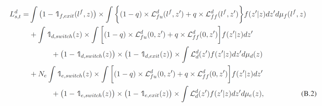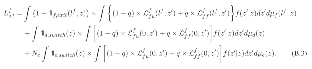In the interest of space, the aggregate variables are defined in Appendix B.

4.4 Numerical Results

We solve the model numerically using a two-step method. In the first step, we solve for the $w_s / p_1$ ratio in sector 1 that satisfies the free entry condition. Specifically, given the $w_s / p_1$ ratio, we iterate the firms’ value functions until the distance between two successive iterations becomes smaller than $10^{-6}$ . Then, if the free entry condition does not hold (e.g., $\left|\mathbb{E}e V^e\left(z{-1}\right)-p_1 c_e\right|>10^{-6}$ ), we revise $w_s / p_1$ and repeat the above step until the free entry condition is satisfied. In the second step, we use the firms’ policy functions we found in the first step to simulate the distribution of the sector 1 firms, calculate the aggregate variables, and check whether the skilled domestic labor market clears. If it does not, we revise the entering mass $N_e$ and repeat the second step until the labor market clears. Last, we calculate expectations using 80 quadrature points for the productivity shock.

4.4.1 Calibration and Functional Forms

We specify the functional form of productivity in sector 1 as $y=f\left(z, l^s\right)=z l^{s \theta}$ , where $\theta$ is the span of control. The foreign labor adjustment cost is set to $\psi\left(l^f, l_{-1}^f\right)=f_r \max \left{l^f-(1-\delta) l_{-1}^f, 0\right}$ . Therefore, the cost is only incurred for the new hiring each period.

For calibrating the model parameters, we adopt an annual calibration such that the stationary equilibrium in the model matches the US economy during 2005–2020. Several parameters are calibrated directly from the data or from findings from prior literature. We set $\beta = 0.96$ , which implies an annual real interest rate of 4 percent. The exogenous return shock to foreign skilled labor is set to $\delta=0.1$ , to match the annual return migration rate of 10 percent (North 2011). We normalize the aggregate skilled domestic labor supply to 1 $\left(L_s=1\right)$ . Given this normalization of skilled domestic labor supply, we then calibrate the unskilled domestic labor supply to $L_u=1.92$ to match the average share of domestic workers with less than a bachelor’s degree, approximately 52 percent, over this time period.

Additionally, we set $q = 0.35$ to match the average fraction of accepted petitions for skilled foreign workers. $\gamma$ is set to be 0.9167 to target an elasticity of substitution between domestic and foreign workers of 12 (Ottaviano & Peri 2012). The span of control $\theta$ is set to 0.97, which is consistent with the estimates in Basu & Fernald (1997) and more recently Gao & Kehrig (2017). Note that $\theta>\gamma$ implies that skilled domestic workers increase the marginal product of skilled foreign workers and vice versa. We set the persistence of the productivity process to $\rho_z=0.6$ and the standard deviation of shocks to $\sigma=0.3$ , consistent with the evidence in Foster et al. (2008) for the high-tech sector, and normalize the average productivity $\mu_z$ to 1.

We calibrate $\alpha=0.485, f_r=0.3, a=1.345, c_e=8.1, c_f=3.41$ , and $c_s=14.3$ to jointly match the targets specified in Table 3. Note that the ratio of regulatory cost $f_r$ to skilled wages $w_s$ is computed using data from the USCIS on average filing costs and data from the CPS on average skilled wages. The average employment in the high-tech sector and average exit rate for firms in this sector are computed from the BDS data. The fraction of type- $f$ firms in the high-tech sector that hire skilled foreign workers is computed as the average proportion of high-tech firms that submit LCAs, and the type- $d$ fraction is just 1− the type- $f$ fraction.¹⁹ $L_f^{\text {demand }}$ refers to the total demand for skilled foreign workers, that is, the sum of demand by the type- $f$ firms that are facing favorable and unfavorable hiring shocks (referred to as type- $ff$ and $fu$ firms) in the model. The corresponding target in the data is computed as the total number of LCAs filed by firms in the high-tech sector (USCIS) as a proportion of total employment in the high-tech sector (BDS). Last, $w_s/w_u$ represents the wage skill premium and is measured using the CPS accessed via IPUMs (Ruggles et al., 2003).

To further evaluate our model, we compare the model-implied distribution of firms across age cohorts with the corresponding distribution in the data for high-tech firms. Note that the distribution was not directly targeted in the calibration. Table 4 shows that our model generates a firm age distribution that is close to the data.

4.5 Counterfactual Policy Exercises

In this section, we implement the following counterfactual policy exercises and compare the equilibrium distributions to the benchmark economy. We first evaluate the impact of the following policy changes on all firms: (1) $q = 1$ (no idiosyncratic hiring frictions), (2) $c_s = 0$ (no sunk costs to switch to type $f$ ), (3) $q = 1$ and $c_s = 0$ , (4) $f_r = 0$ (no per-worker hiring cost), and (5) no immigration policy frictions ( $q = 1$ , $c_s = 0$ , and $f_r = 0$ ).

To study the impacts of lower immigration frictions on all firms, Table 5 expresses the stationary equilibrium of the economies under cases (1)–(5) relative to the benchmark economy. Note that a higher $q$ , a lower $c_s$ , or a lower $f_r$ reduces the foreign worker hiring barriers for firms, thus increasing the total number of skilled foreign workers $L_s^f$ in the stationary equilibrium. As expected, the impacts are the largest in the completely frictionless case for all firms, that is, case (5). The higher influx of skilled foreign workers in turn boosts sector 1’s output and its consumption $Y_1$ , which is the production net of costs.

The greater value of sector 1 consumption goods pushes down the prices of sector 1 goods ( $p_1$ ) and boosts the relative price of sector 2 goods ( $p_2$ ). As a result, skilled-intensive sector wages $w_s$ decrease, and unskilled sector wages $w_u$ rise. Consequently, skilled domestic households experience a reduction in consumption, and unskilled domestic households enjoy a higher consumption from lax skilled immigration policies. Note that the complementarity between skilled and unskilled workers in the model arises through the consumption basket. On the other hand, lower immigration policy frictions encourage more firms to enter the market and enjoy the benefits of hiring foreign workers. In the equilibrium with no immigration policy frictions, the mass of firms is approximately 56 percent higher compared to the baseline economy. The frictionless counterfactual witnesses a more than 14-fold increase in the aggregate skilled foreign labor stock, a 26 percent higher aggregate skilled-intensive output, and a 66 percent higher new firm entry.

To explore the impacts of our counterfactual policy by firm age cohorts, Figure 5 plots the average sector 1 variables by firm age in the benchmark economy and under the cases with no immigration frictions. Note that Appendix Figure C.4 plots the corresponding averages for the other cases, which are qualitatively similar but have less of a quantitative than the completely frictionless cases.

First, consider the intuition behind the average variables by age in the benchmark case. Firms draw the initial productivity after deciding to enter the market and may choose to exit immediately after observing the draw. Therefore, around 14 percent of the firms exit immediately after entering, and only those with high initial productivity stay. Since the productivity process is persistent, only firms with very unfavorable productivity shocks in the subsequent periods choose to exit, resulting in a lower exit rate in periods after the initial period. As firms become older, only those with greater productivity levels survive, pushing up the average total factor productivity among the surviving firms. It is also intuitive that older firms have higher average skilled workers (skilled foreign or domestic workers), higher average production, and a smaller fraction of type- $d$ firms among older firms.

Reflecting on this, we use Figure 5 to compare the firm averages by age in the benchmark case with the corresponding averages under the case with no immigration frictions ( $q = 1, c_s = 0$ , and $f_r = 0$ ).
Interestingly, eliminating frictions has a similar effect on both the average exit rate and average productivity. Lower immigration policy frictions increase the average exit rate for older firms and increase their average productivity, which pushes up the average productivity of all firms in the economy. The average productivity in the case with no immigration policy frictions is approximately 0.4 percent higher than in the benchmark case. Consistent with our empirical evidence, lower immigration policy frictions also increase the survival of younger firms and decrease their exit rates. Intuitively, a higher new firm entry and young firm survival push out less productive incumbents, leading to higher average exit rates for older firms and higher average productivity. As a result, the higher exit rate is also accompanied by a higher entering mass, leading to a bigger firm mass in equilibrium, as shown in Table 5. This result is also consistent with the fact that the exit rate among older firms declined after immigration policies were tightened in 2005, as we will discuss in the next section.

Figure 5. Average Firm Characteristics by Age

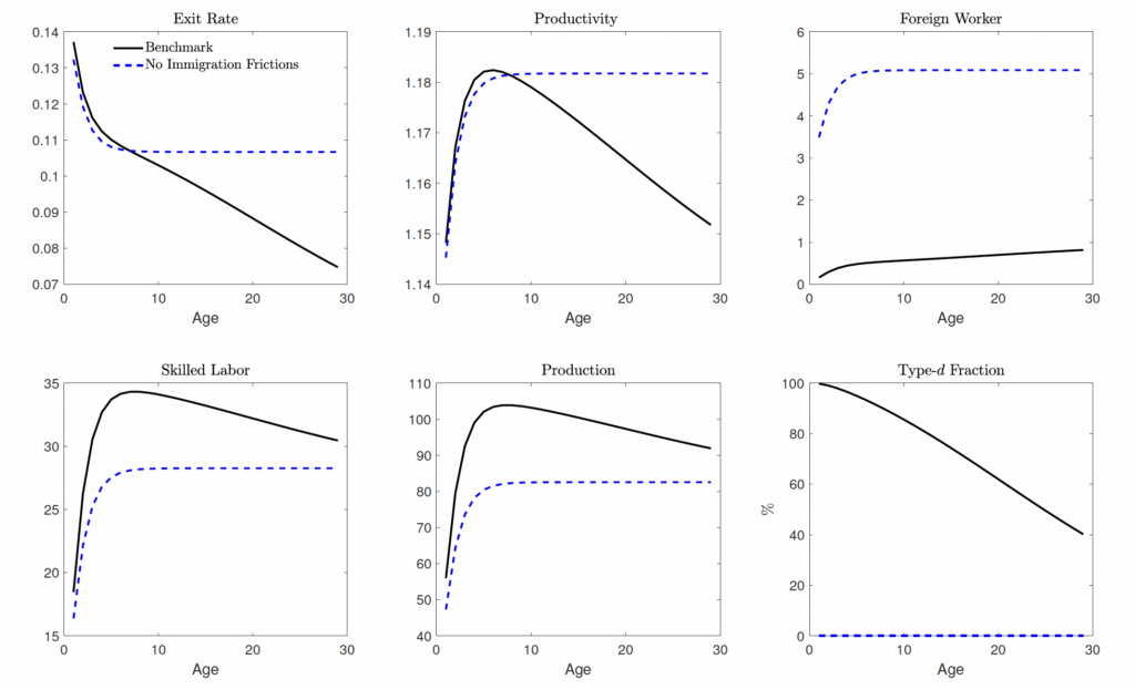
In addition, lower immigration policy frictions reduce the barrier to acquiring foreign workers and result in more skilled foreign workers for firms of all ages. Moreover, since the mass of firms is higher in the frictionless case, the average production and average skilled labor employed per firm are lower. Therefore, even though the aggregate output of sector 1 increases, the average production of each firm is smaller due to the larger firm mass.

To summarize, lower immigration policy frictions lead to more firms entering, a higher mass of firms, and more foreign workers. The increase in aggregate output for sector 1 leads to a decrease in the sector’s
overall price $p_1$ and an increase in the cost of production ( $w_s/p_1$ ). Therefore, less productive firms are more likely to exit, and the average productivity increases in the economy.

Extensive and intensive margins. In this section, we examine the effects of these immigration policy changes by the extensive versus the intensive margin. Table 5 shows that a relaxed immigration policy reduces the costs of hiring foreign workers, resulting in a higher mass of firms in equilibrium. Therefore, a fraction of the skilled domestic workers can be considered hired by these “additional” firms, which we interpret as the extensive margin. To separate the effects by the intensive and extensive margin, we “ration” the skilled labor so that each worker supplies labor that is smaller than one. Due to the rationed skilled domestic labor market, the wages of skilled workers become higher, reducing the firm value and causing the firm mass to decline. We then search for the fraction of skilled domestic labor that must be rationed to reduce the firm mass back to the baseline case.

Table 6 shows the effects of removing all immigration frictions and the case with a fixed mass of firms
through a rationed labor market, where all numbers are reported relative to the baseline case.²⁰ As shown in the first row, 36.5 percent of the domestic workers are hired by the additional firms induced by the lower immigration frictions. In the case of rationed skilled domestic labor (thus a fixed firm mass), the consumption of skilled domestic workers is only 72.6 percent of the level in the baseline case, indicating that fully relaxed immigration frictions would reduce the welfare of skilled domestic workers by 27.4 percent by the intensive margin. On the other hand, the total effects (including both the extensive and intensive margins) of relaxed immigration policies reduce the welfare of skilled domestic workers by 9.5 percent, indicating a 17.9 percent increase in the welfare of these workers by the extensive margin relative to the baseline case.

Similarly, a relaxed immigration policy reduces the welfare of domestic unskilled workers by 10.01 percent by the extensive margin. It also increases their welfare by 22.1 percent by the intensive margin,
resulting in a total welfare gain of 12 percent for these workers.

5 Policy Implications and Conclusion

The results in the previous section show that reducing skilled immigration policy regulations—for instance, by simplifying procedures to lower sunk costs or reducing filing fees and idiosyncratic frictions due to the lottery process—can play an important role in increasing business dynamism in technology-intensive sectors. This is achieved by increasing the mass of younger firms and pushing out older, less productive ones. Eventually, such changes would increase the average productivity of operating firms.

We now highlight two trends observed in high-tech sectors since 2005 that are broadly consistent with our model mechanisms. Note that the period after 2005 can be interpreted as one with higher immigration policy frictions after the H-1B visa cap was reduced in 2004 (Figure 3). First, the period after 2005 was associated with lower average exit rates of older firms in the high-tech sector, compared to the period between 1990 and 2004 (Figure 6).²¹ This is consistent with the mechanism of our general equilibrium model (Figure 5)—higher immigration policy frictions would reduce the average exit rate of older firms in the economy. Second, there has been an increase in the share of the smallest firms (least productive firms with 1–19 workers) within the oldest firms (age 11+) in the high-tech sector, as seen in Figure 2.²² This trend is also consistent with our model mechanism—higher immigration frictions would reduce the mass of entering firms and lead to an increase in the survival of older, less productive firms.

Figure 6. Firm Exit Rate by Firm Age

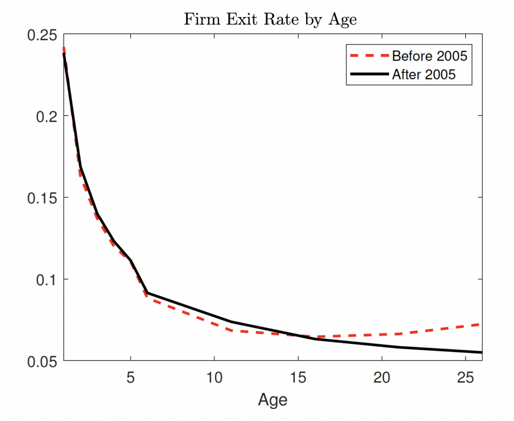
In summary, our model predictions are not inconsistent with trends observed in the data since 2005 after immigration policies became more restrictive—a lower average exit rate of older firms and an increase in less productive (smaller) firms within the older firms. While there are many other factors that have contributed to these phenomena since the early 2000s, immigration policy restrictions may have played a role in influencing these trends in the high-tech sector, consistent with our model implications. The empirical relationships between immigration policies and firm dynamics by firm age in tech-intensive sectors have been previously ignored and require closer investigation beyond the scope of this paper. However, this paper establishes that skilled immigration policy frictions directly influence the dynamics of young firms in the high-tech sector by impacting firm survival. Additionally, it reveals important general equilibrium impacts of these frictions on firms across age cohorts and on the overall average productivity of firms.

Appendix

A H-1B Program: Institutional Framework and Background

Since the H-1B visa program was implemented in 1990, it has been the main method of entry into the US workforce for foreign college-educated professionals. The H-1B visa is temporary as it is issued for only three years (and can be renewed for another three), but it is a dual intent visa since it can lead to permanent residency if the employer is willing to sponsor the worker for a green card.

The H-1B program has been subject to an annual quota on new visa issuances. The initial visa cap was 65,000, which was subsequently increased to 115,000 in 1999 and 2000 after the cap was met in 1997. The cap was further increased to 195,000 from 2001 to 2003. In 2001, cap exemptions were introduced for employees at higher education, nonprofit, and government research organizations. In 2004, the cap was reduced back to 65,000, but 20,000 additional visas were allocated for workers who had obtained a master’s degree or higher from a US institution. The cap applies only to new H-1B visa issuances for for-profit firms.

To obtain an H-1B visa, there are several steps to be followed, and firms are central to this process. The first step requires the firm that wants to hire a foreign worker to file an LCA with the Department of Labor. In the application, the firm specifies the nature of the worker’s occupation and attests that it will pay them the greater of the actual compensation paid to other employees in the same job or the prevailing compensation for that occupation. The rationale given for this attestation is to help protect domestic worker wages. The LCA request also certifies that the employer must hire a foreign worker because a US citizen is not qualified, available, or willing to work in that job position.

LCA forms can request one or more foreign workers for a particular occupation, and thus they signal firm vacancies in specific occupations for foreign workers. LCAs are processed relatively quickly, allowing firms to file them either after hiring workers or in anticipation of hiring. However, there are some limitations of using the LCA database. The database contains records for every request submitted, but this is only an intermediate step in the process toward the final visa approval. An LCA is submitted for every H-1B request, whether new or a renewal, and each LCA can contain multiple H-1B workers.

Once the Department of Labor approves the LCA, it is sent to the USCIS along with the I-129 form²³ and the required visa fees. This is the final step, and firms have from April 1 until the beginning of the next fiscal year to file petitions for H-1B visa applications. Crucially, potential employees can only apply for an H-1B visa if they have a job offer from an employer with LCA approval. By law, the employer cannot file more than one I-129 for the same prospective employee. Most of the filing and legal fees are also borne by the employer. If the number of H-1B visa petitions (I-129 forms) that fall within the nonexempt category exceeds the cap, the USCIS randomly selects visas for processing via a lottery system until the 65,000 cap is reached. The total number of petitions filed does not indicate the true demand because the government stops collecting H-1B petitions once it has determined that the cap has been reached for a given year.

In recent years, the Department of Homeland Security has been considering amendments in its regulations regarding the process by which the USCIS selects H-1B petitions for the filing of the H-1B cap-subject petitions. In 2020, the USCIS implemented a preregistration process that begins on March 1 for potential employees who want to file an H-1B petition. If the USCIS receives enough registrations by March 18 (based on historic projections), they will randomly select registrations. An H-1B cap-subject petition may only be filed by a petitioner whose registration was selected (also see Pathak et al., 2022 for an extensive analysis of the H-1B rule changes over the years). In very recent years there have also been increasing cases of fraud and multiple registrations submitted for the same employee. However, such cases are subject to legal actions. The USCIS mentions that “based on evidence from the FY 2023 and FY 2024 H-1B cap seasons, USCIS has already undertaken extensive fraud investigations, denied and revoked petitions accordingly, and continues to make law enforcement referrals for criminal prosecution.”²⁴

B Aggregation

This section discusses how the aggregate variables are calculated using the firm’s distributions. The aggregate output of sector 1 is given by

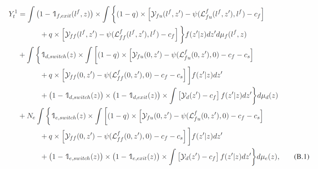
where $\mathcal{Y}_{f f}\left(l^f, z^{\prime}\right)$ and $\mathcal{L}_{f f}^f\left(l^f, z^{\prime}\right)$ are the production and foreign worker hiring decisions for a type- $f$ firm that (1) just received a positive hiring shock, (2) has number $l^f$ of foreign workers at the beginning of the period, and (3) just drew productivity $z^{\prime}$ after observing productivity $z$ and making the exit decision. $y_{f u}\left(l^f, z^{\prime}\right)$ and $\mathcal{L}_{f u}^f\left(l^f, z^{\prime}\right)$ are similarly defined. $\mathcal{Y}_d\left(z^{\prime}\right)$ and $\mathcal{L}_d^f(z)$ are the production and foreign worker hiring decisions for a type- $d$ firm that just drew productivity $z^{\prime}$ after observing productivity $z$ and making the switch/exit decision. $\mathbb{1}_{f, \text { exit }}\left(l^f, z\right)$ , $\mathbb{1}_{d, \text { exit }}(z)$ , and $\mathbb{1}_{e, \text { exit }}(z)$ are the exit decisions for the type- $f$ , typed, and entering firms. $\mathbb{1}_{d, \text { switch }}(z)$ and $\mathbb{1}_{e, \text { switch }}(z)$ are the switch decisions made by the type- $d$ firms and entering firms with productivity $z$ . $N_e$ is the mass of new entries, and $f\left(z^{\prime} \mid z\right)$ is the transition probability of the idiosyncratic productivity shock.

The aggregate skilled domestic worker is given by

where $\mathcal{L}_{f u}^d$ , $\mathcal{L}_{f f}^d$ and $\mathcal{L}_d^d$ are the hiring decisions for skilled domestic workers made by each type of firm. Similarly, the aggregate skilled foreign worker is given by

C Additional Figures and Tables

Figure C.1. Number of Young Firms between 1986 and 2020

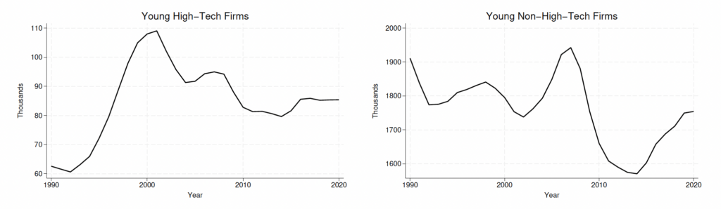
Notes: The figure is compiled using the US Census Bureau’s BDS. High-tech firms are computed using four-digit NAICS codes and the BLS classification (Heckler, 2005).

Figure C.2. Share of Young Firms

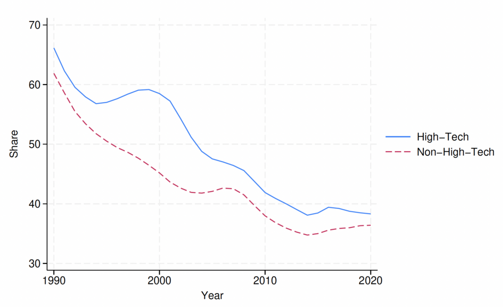
Notes: The figure is compiled using the US Census Bureau’s BDS. High-tech firms are computed using four-digit NAICS codes and the BLS classification (Heckler, 2005).

Figure C.3. Share of Largest Firms (500+ Employees) in Oldest Age (11+) Cohorts

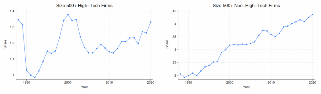
Notes: The figure is compiled using the US Census Bureau’s BDS. Left (right) panel corresponds to the high-tech sector (non-high-tech sector). High-tech firms are computed using four-digit NAICS codes and the BLS classification (Heckler, 2005).

Figure C.4. Average Firm Characteristics by Age

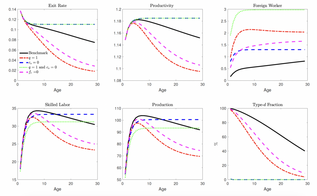
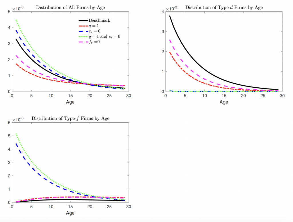
Figure C.5. Firm Distribution by Age

References

Barnatchez, K., Crane, L. D., & Decker, R. (2017). An assessment of the national establishment time series (NETS) database.

Basu, S., & Fernald, J. G. (1997). Returns to scale in US production: Estimates and implications. Journal of Political Economy, 105(2), 249–283.

Bento, P., & Restuccia, D. (2017). Misallocation, establishment size, and productivity. American Economic Journal: Macroeconomics, 9(3), 267–303.

Bound, J., Braga, B., Golden, J. M., & Khanna, G. (2015). Recruitment of foreigners in the market for computer scientists in the United States. Journal of Labor Economics, 33(S1 Part 2), S187–S223.

Bound, J., Khanna, G., & Morales, N. (2017). Understanding the economic impact of the H-1B program on the US. In High-Skilled Migration to the United States and its Economic Consequences. University of Chicago Press.

Brinatti, A., Chen, M., Mahajan, P., Morales, N., & Shih, K. Y. (2023). The impact of immigration on firms and workers: Insights from the H-1B lottery. Available at SSRN 4431106.

Clementi, G. L., & Palazzo, B. (2016). Entry, exit, firm dynamics, and aggregate fluctuations. American Economic Journal: Macroeconomics, 8(3), 1–41.

Decker, R. A., Haltiwanger, J., Jarmin, R. S., & Miranda, J. (2016a). Declining business dynamism: What we know and the way forward. American Economic Review, 106(5), 203–207.

Decker, R. A., Haltiwanger, J., Jarmin, R. S., & Miranda, J. (2016b). Where has all the skewness gone? The decline in high-growth (young) firms in the US. European Economic Review, 86, 4–23.

Dimmock, S. G., Huang, J., & Weisbenner, S. J. (2021). Give me your tired, your poor, your high-skilled labor: H-1B lottery outcomes and entrepreneurial success. Management Science.

Doran, K., Gelber, A., & Isen, A. (2016). The effects of high-skilled immigration policy on firms: Evidence from visa lotteries.

Foster, L., Haltiwanger, J., & Syverson, C. (2008). Reallocation, firm turnover, and efficiency: Selection on productivity or profitability? American Economic Review, 98(1), 394–425.

Gabler, A., & Poschke, M. (2013). Experimentation by firms, distortions, and aggregate productivity. Review of Economic Dynamics, 16(1), 26–38.

GAO. (2011). H-1B visa program: Reforms are needed to minimize the risks and costs of current program.

Gao, W., & Kehrig, M. (2017). Returns to scale, productivity and competition: Empirical evidence from US manufacturing and construction establishments. Productivity and Competition: Empirical Evidence from US Manufacturing and Construction Establishments (May 1, 2017).

Glennon, B. (2020). How do restrictions on high-skilled immigration affect offshoring? Evidence from the H-1B program (Tech. Rep.). National Bureau of Economic Research.

Haltiwanger, J., Hathaway, I., & Miranda, J. (2014). Declining business dynamism in the US high-technology sector. Available at SSRN 2397310.

Heckler, D. E. (2005). High-technology employment: a NAICS-based update. Monthly Labor Review, 128, 57.

Hopenhayn, H. (1992). Entry, exit, and firm dynamics in long run equilibrium. Econometrica: Journal of the Econometric Society, 1127–1150.

Hopenhayn, H., & Rogerson, R. (1993). Job turnover and policy evaluation: A general equilibrium analysis. Journal of Political Economy, 101(5), 915–938.

Kerr, S. P., Kerr, W. R., & Lincoln, W. F. (2013). Skilled immigration and the employment structures of US firms (Tech. Rep.). National Bureau of Economic Research.

Kerr, S. P., Kerr, W. R., & Lincoln, W. F. (2014). Firms and the economics of skilled immigration. In Innovation Policy and the Economy, Volume 15. University of Chicago Press.

Kerr, W. R., & Lincoln, W. F. (2010). The supply side of innovation: H-1B visa reforms and US ethnic invention. Journal of Labor Economics, 28(3), 473–508.

Mahajan, P. (2022). Immigration and business dynamics: Evidence from US firms.

Mehra, M., & Kim, D. (2023). Skilled immigration, offshoring, and trade. Journal of Economic Dynamics and Control, 146, 104579.

Mehra, M., & Shen, H. (2022). Skilled immigration, firms, and policy. Journal of International Economics, 103662.

Mukoyama, T., & Osotimehin, S. (2019). Barriers to reallocation and economic growth: The effects of firing costs. American Economic Journal: Macroeconomics, 11(4), 235–270.

North, D. (2011). Estimating the size of the H-1B population in the US. Center for Immigration Studies Memorandum.

Olney, W. W. (2013). Immigration and firm expansion. Journal of Regional Science, 53(1), 142–157.

Orrenius, P. M., Zavodny, M., & Abraham, A. T. (2020). The effect of immigration on business dynamics and employment.

Ottaviano, G. I., & Peri, G. (2012). Rethinking the effect of immigration on wages. Journal of the European Economic Association, 10(1), 152–197.

Ottaviano, G. I., Peri, G., & Wright, G. C. (2018). Immigration, trade and productivity in services: Evidence from UK firms. Journal of International Economics, 112, 88–108.

Pathak, P. A., Rees-Jones, A., & Sönmez, T. (2022). Immigration lottery design: Engineered and coincidental consequences of H-1B reforms. Review of Economics and Statistics, 1–43.

Peri, G., Shih, K., & Sparber, C. (2015a). Foreign and native skilled workers: What can we learn from H-1B lotteries? (Tech. Rep.). National Bureau of Economic Research.

Peri, G., Shih, K., & Sparber, C. (2015b). STEM workers, H-1B visas, and productivity in US cities. Journal of Labor Economics, 33(S1), S225–S255.

Peri, G., Shih, K. Y., & Sparber, C. (2014). Foreign STEM workers and native wages and employment in US cities (Tech. Rep.). National Bureau of Economic Research.

Ranasinghe, A. (2014). Impact of policy distortions on firm-level innovation, productivity dynamics and TFP. Journal of Economic Dynamics and Control, 46, 114–129.

Raux, M. (2023). Looking for the best and brightest. The Center for Growth and Opportunity.

Ruggles, S., King, M. L., Levison, D., McCaa, R., & Sobek, M. (2003). IPUMS-international. Historical Methods: A Journal of Quantitative and Interdisciplinary History, 36(2), 60–65.

Sedláček, P. (2020). Lost generations of firms and aggregate labor market dynamics. Journal of Monetary Economics, 111, 16–31.

Waugh, M. E. (2018). Firm Dynamics and Immigration. In High-Skilled Migration to the United States and Its Economic Consequences. University of Chicago Press.

Skilled Immigration Frictions as a Barrier for Young Firms

Executive Summary

Resources

Focuses

1 Introduction

3 Empirical Evidence