On the Design of an Optimal Immigration Policy

Lopez-Velasco, Armando R.

1 Introduction

What does an optimal immigration policy look like? This question has received little attention in the literature of immigration.¹ Perhaps part of the explanation is that, as Chassamboulli and Peri (2020, p. 1) put it, ”Economists have adopted, so far, rather simplified models to evaluate the consequences of changing immigration policies on the national economy and labor markets. Usually they have analyzed the consequences of a change in the number and in the composition of foreign-born as shifts in supply within a neoclassical model.” Those carefully estimated models are clearly useful for many purposes, but they are not designed to explain why certain immigration channels exist in the first place or what an optimal immigration policy looks like.

To fill this gap, the current paper introduces a new model for the study of optimal immigration. This model can explain the existence of two common immigration categories in the US, i.e., family-based immigration and employment-based (skill-based immigration), as well as an unauthorized immigration channel. Together, these channels represent the majority of the immigration flows to the US.²

One of the advantages of understanding these immigration categories is that the results of this study are to some extent easier to relate to policy than if the model considered the ”skilled” and ”unskilled” immigration groups typically studied. For example, the current framework could be used to study the implications of having a more skill-based immigration system. Though many researchers (e.g. Borjas (2001)) and politicians have argued in its favor in previous years, it is not clear how to accomplish such a policy when the majority of US immigration permits are currently awarded to family-based immigrants. Does this translate into giving more permits to skill-based immigration while not affecting family-based? Or does it mean that permits available for family-based immigration should be reduced? The current framework can offer a possible answer to this and other policy-relevant questions.

In the model, the native majority optimally chooses quotas of skill-based and family-based immigrants as well as the level of enforcement expenditure, which in turn helps to determine the equilibrium level of unauthorized immigration. The type and quantity of allowed immigrants both affect the size of a transfer available to all agents, as well as the amount of a public good subject to congestion in the host country. The natives’ welfare depends on (i) the size of the transfer per person, (ii) the level of family-based immigration, and (iii) the amount of the common resource available per person. There are three types of immigrant groups from which the host economy can choose whether and if so how many of them to allow into the country: skill-based immigrants, whose productivity is the highest among the different types; immigrants with family ties to natives; and unauthorized or illegal immigrants who are able to evade or are not deterred by the enforcement technology.

The paper presents three conditions that jointly characterize optimal immigration. The first condition balances skill-based with family-based immigration, where those in the former group are allowed into the country because their fiscal contributions are larger than those of family-based immigrants, who provide utility from reunification instead. The second condition balances the external effects on transfers against the congestion externalities on the public good. The third condition dictates the optimal level of enforcement, obtained by equating the fiscal opportunity cost of unauthorized immigrants, relative to the contributions of skill-based immigrants, with the marginal cost of enforcement. These conditions are new in the literature.

This model is robust along several dimensions. The assumption of a social welfare function summarizes a more elaborate political process where natives with heterogeneous preferences over the modeled issues can be justified under probabilistic voting arguments (Lindbeck and Weibull (1987)) and is typically used in analysis of optimal policies. The model considers both legal and illegal immigration as their fiscal effects are different (e.g. Blau and Mackie (2017)). The fiscal constraint of the model with the enforcement technology can be derived under closed- or open-economy interpretations, and the model can incorporate a second public good that is produced under a constant returns to scale technology that is paid by tax revenue. For simplicity of exposition, the extensions and alternative derivations are relegated to the Appendix (sections A.4 to A.7).

The model is calibrated for the period 1994-2008, a span also used by Guerreiro, Rebelo, and Teles (2020), under two alternative assumptions. The baseline calibration assumes that observed immigration flows are optimally determined by the host country, while an alternative calibration assumes that they are sub-optimal due (for example) to a political constraint on skill-based immigration, something that could arise in the case of the US if the current cap on the number of employment-based visas is too low. In either case, the analysis reveals that family-based immigration is not responsive to economic or demographic shocks, other than to changes in their productivity and therefore their fiscal contributions. In turn, unauthorized immigration increases in response to a bigger supply of potential unauthorized immigrants or in response to increases in the immigrants’ own productivity, among other effects.

The model in the baseline calibration uses skill-based immigration as a ”shock-absorber”: additional skill-based immigration helps ameliorate the detrimental fiscal effects from the lower productivity of family-based or unauthorized immigrants, or in response to an increase in the supply of unauthorized immigration. This is somewhat similar to Storesletten’s (2000) result, where selective immigration policies (mostly skill-based immigration) can be used to sustain fiscal policies in the presence of fiscal imbalances.

In the model with constrained skill-based immigration, unauthorized immigration is not contained as much as when skill-based immigration can increase. In this case, skill-based immigration becomes insensitive to most economic and demographic factors, as opposed to decreasing when the productivity of unauthorized or family-based immigrants increases, for example.

There are two particular forces that stand out during the period of consideration. First, the skill premium increased during this period (see Acemoglu and Autor (2012)). Second, the flows of unauthorized immigration to the US increased significantly relative to the previous two decades, going from about 225,000 new unauthorized immigrants in the 1980s (Smith and Edmonston (1997)) to about 500,000 new unauthorized immigrants during the discussed period. This sustained increase in unauthorized immigration coincided with nearly tripled government spending on enforcement, as measured by the border patrol budget as a percentage of GDP. Higher enforcement expenditure and higher unauthorized immigration are predicted effects of an increase in the supply of potential unauthorized immigrants.

Other facts about this period offer additional evidence of a bigger pool of potential unauthorized immigrants responding to ”pull” and ”push” factors. First, the growth rate of income per capita in the US was larger than the average for Latin America and Caribbean countries (30.4% vs 26.5%), the two main sending regions for unauthorized immigrants. Likewise, during this period the unemployment rate in the US was approximately 3 percentage points lower than the average unemployment rate for the sending countries, while in the early 1990s the US unemployment was higher. Finally, the population growth rate of the 15-64 age-group grew faster in the sending countries than in the US (31.3% vs 18.4%).

The model can be used to interpret the above effects given some assumptions about the quantification of the pool of unauthorized immigrants, as this variable is not directly observable. The optimal response to both changes is to significantly increase skill-based immigration, to keep family-based immigration approximately unchanged, and to increase enforcement expenditure. Unauthorized immigration is affected in opposite directions. Higher productivity among skilled-based immigrants would decrease it, while a higher supply of potential unauthorized immigration would increase it. The second effect dominates and thus predicts an increase in the flow of unauthorized immigration.

US immigration policy has established an annual cap of 140,000 permanent residence permits available for employment-based immigration since 1990.³ But during the analyzed period there were several projects of comprehensive immigration reform which would have given a much more important role to this type of immigration and which perhaps for other political reasons none became law.⁴ Those legislative proposals are largely consistent with the predictions of the model as they didn’t modify family-based immigration, added a very significant increase in skill-based permits, in addition to addressing enforcement.

In light of the above discussion, the model in the baseline calibration can be interpreted as ”what policy would natives prefer?”, while the calibration under the stringent cap on skill-based immigration is a possible interpretation of ”what could explain what happened during this period?”.

The paper is organized as follows. Section 2 places the paper in the literature. Section 3 discusses some of the relevant history of immigration laws governing immigration in the US. Section 4 introduces the model, characterizes the optimal immigration policies, and presents an analytic solution and its comparative statics. Section 5 presents the two alternative calibrations for the US, depending on whether the immigration flows are assumed to be optimal or suboptimal, performs some experiments, and analyzes the demand for US immigration reform through the lens of the model. Section 6 presents some sensitivity analyses. Section 7 discusses some additional policy issues, then Section 8 concludes.

This paper is related to several strands in the literature. First, it is related to politico-economic models of immigration where the equilibrium immigration policy is politically determined since immigration affects, or interacts with, other economic issues. This literature includes studies by Haupt and Peters (1998) and Sand and Razin (2007) on immigration and social security, work by Dolmas and Huffman (2004) as well as the several models of Razin, Sadka, and Suwankiri (2011) on immigration and redistribution, research by Ortega (2005) and Bohn and Lopez-Velasco (2018) on how immigration affects the current and future skill-composition of the country, and work by Bohn and Lopez-Velasco (2019) on immigration policy when immigrants have higher fertility rates. The current paper contributes to this strand by considering immigration categories in line with those observed in the US and other countries, which illustrates new trade-offs and which are relatively easier to relate to policy than other models in the literature.

The paper is also related to previous literature related to unauthorized immigration and enforcement. The seminal paper is Ethier (1986), which analyzes this issue under a costly enforcement technology. Other notable contributions to this literature include Bond and Chen (1987), which generalizes Ethier’s model to two countries, and more recently Bandyopadhyaya and Pinto (2017), which generalizes these models along several lines in order to investigate unauthorized immigration and the degree of decentralization in immigration enforcement policies. The paper by Guzman, Haslag and Orrenius (2008) considers equilibrium unauthorized immigration under an explicit smuggling technology. For empirical papers on this topic, please see the references in Bandyopadhyaya and Pinto (2017). These and other papers in the literature obtain results for unauthorized immigration while ignoring interactions with other types of immigration and thus represent ”optimal enforcement” policies. The present paper complements this literature by studying optimal enforcement in the presence of the other immigration categories, where a different trade-off is identified.

The paper is also related to a relatively small literature that studies the economic outcomes of family-based immigration. This topic has not received much attention, perhaps because typical datasets do not distinguish the type of entry permit that immigrants used (OECD (2017)), even though the majority of permits in the US and other developed countries are for family-based immigration. One of the few papers in this literature is Aydemir (2011), which finds that labor-based immigration using the point system in Canada leads to selecting immigrants with much higher skill levels than those under family preferences. The OECD (2017, p. 9) reports that ”the few available studies show that the outcomes of family migrants are less favorable than those of labour migrants.” Finally, the paper by Chassamboulli and Peri (2020) models family-based immigration, in addition to employment-based and unauthorized immigration, with a search-matching model that allows the authors to analyze realistic policy changes on the equilibrium immigration of the different types. The current paper is informed by this literature and complements it by constructing a model that can theoretically explain the demand for family-based immigration and its trade-offs with skill-based immigration.

Very few papers have considered what an optimal immigration policy looks like— in fact, only two other studies have formally defined this question with the rigor of an economic model. The first one is by Benhabib and Jovanovic (2012), who derive optimal immigration policies at the world level. Their modeling strategy differs from the current paper as it is focused on the optimal distribution of the world population. The other paper, Guerreiro, Rebelo, and Teles (2020), studies optimal immigration from the natives’ perspectives in the presence of both an optimal redistributive welfare system and external effects of immigration. The current paper has similarities to these papers, as it considers a static model and maximizes a social welfare function, but it addresses different questions in an effort to understand all three categories of immigration (family-based, skill-based, and unauthorized), as well as their interdependence in the optimal policy.

One of the contributions of this paper is to offer an answer as to why a country would design an immigration system along the lines of the US system and which is also a staple of many other countries (OECD (2017)). This is done by constructing a model that is calibrated for the US experience.

Another contribution of this paper is to offer this model as an analytical framework for certain policy questions, including the optimal response to certain economic and demographic changes. For example, should family-based immigration be reduced from current levels? According to the model, it depends. If the net fiscal contributions of family-based immigrants are reduced (say because exogenously, their productivity is lower or their net fiscal contributions decrease), then the answer is yes, and at the same time the country should increase skill-based immigration. But should family-based immigration decrease because of higher productivity of skill-based immigrants? Or should it decrease because unauthorized immigration increases as a result of a bigger supply of unauthorized immigrants? In both cases the answer is no: skill-based immigration should be increased without affecting the family-based category. These type of questions would be harder to answer if the model only considered skilled and unskilled categories. Furthermore, the model could be generalized along several dimensions to consider other issues in the literature.

As many developed countries cannot choose new fiscal policies from scratch, since doing so would likely require reneging on existing fiscal promises, the current model is suitable for the study of immigration reform as a single political item, without considering significant changes to other instruments of fiscal policy— similar to immigration reform projects presented in the US (see Section 5.3) in previous years.

3 A Brief History of US Immigration Policy

With few exceptions, immigration to the US was mostly unregulated prior to 1900. Starting in 1875 several laws were passed that banned particular groups: polygamists, sick people, the Chinese and then Asians in general, anarchists, and importers of prostitutes, among others. Then in 1921 the Emergency Quota Act was passed, which instituted quota limits of 3% of the foreign-born population of any given nationality in the 1910 census, but which didn’t apply to countries in the Western Hemisphere. These quotas were revised to 2% with reference to the 1890 census through the Immigration Act of 1924, which continued to bar immigration from Asia. These efforts were put in place to support existing immigration patterns. The Labor Appropriation Act, also passed in 1924, created the Border Patrol to address illegal immigration and smuggling.

In 1952, the quotas by origin were updated and new categories for skilled immigration and family reunification were created. Then the 1965 Immigration and Nationality Act replaced the old nationality-quota system with a system that favored family-reunification and immigrants with certain skills. Modern immigration categories are in large part determined by this law.

Another significant piece of legislation was the 1986 Immigration Reform and Control Act, which was passed in response to growing unauthorized immigration to the US and which provided a path for unauthorized immigrants to legalize their status. It also legalized a total of 2.7 million previously unauthorized immigrants, increased the tools for border enforcement, and provided for sanctions against employers who hired undocumented workers (Wasem (2014)).

Current limits on annual permits are inherited from the Immigration Act of 1990, which established a cap of 675,000 annual permits starting in 1995 (but provided a slightly larger number of 700,000 from 1992 to 1994). This number can be surpassed as there are no limits on immigration by immediate relatives of US citizens, even while limiting immigration of the other categories.

For a more detailed summary of these laws, including smaller and more recent reforms like the Secure Fence Act in 2006 and the Deferred Action for Childhood Arrivals – DACA in 2012, see Cohn (2015) or the Migration Policy Institute (2013). For a detailed analysis of the unintended consequences of the 1965 Immigration and Nationality Act, see Massey and Pren (2012).

4 The Model

Let immigration quotas be defined as $\theta_{i}\equiv\frac{M_{i}}{N},$ where $M_{i}$ is the number of immigrants of type $i=\left{ S,F,U\right}$ and $N$ is the number of natives. Immigration type $S$ represents skilled-based immigration, type $F$ represents family-based immigration, and type $U$ represents unauthorized immigration.

The fiscal side of the model is captured in a simple way by assuming that the government runs a balanced budget where taxes on wages are used to pay transfers and the enforcement expenditure. All natives, skill-based immigrants, and family-based immigrants pay an exogenously constant tax rate $\tau$ , with $0<\tau<1$ . In the case of unauthorized immigrants, the government taxes a fraction $0<\lambda\leq1$ of their income and thus they pay the tax rate $\lambda\tau\leq\tau.$ Collected taxes are used to pay for the cost of immigration enforcement, defined in terms of cost-per-native as $E$ , as well as to finance a transfer $b$ to natives and all legal immigrants. Unauthorized immigrants do not receive the full benefit $b$ , but receive $(b-\eta)$ , where $0\leq\eta<b$ represents some savings in transfers as unauthorized immigrants typically do not qualify for all benefits.⁵

The equation summarizing these ideas is given by

(1) $\begin{equation*}\tau\left( w+w_{F}\theta_{F}+w_{s}\theta_{s}+\lambda w_{u}\theta_{u}\right)=b\left( 1+\theta_{F}+\theta_{s}\right) +\left( b-\eta\right) \theta_{u}+E, \end{equation*}$

where $w$ , $w_{F},$ $w_{s}$ and $w_{u}$ are the wages of natives, family-based immigrants, skill-based immigrants, and unauthorized immigrants, respectively.

Wages $\left{ w,w_{F},w_{s},w_{u}\right}$ are assumed to be constant and not affected by the immigration flows, an assumption that requires discussion. First, this is consistent with a long-run interpretation of the model where the labor inputs are perfect substitutes for different levels of efficiency. In the long run, capital (if the model were to include capital) adjusts so that wage effects due to a possible dilution of capital are zero, and the so-called “immigration surplus” would also be zero. This is consistent with the empirical literature that finds mixed evidence on the wage effects of immigration.⁶ Second, it is also consistent with the short run under a small open economy interpretation with perfect substitution among the labor inputs.

Lastly, assuming imperfect substitution among the labor inputs can produce distributional effects of immigration. But incorporating them into the model produces a different problem: it would imply that immigrants permanently change the wage premiums, something inconsistent with the changing incentives of a different wage premium in the long run (e.g., changing occupations or acquiring human capital in response to wage effects). Because of these reasons and to keep the model tractable, the wage effects of immigration are ignored.⁷

The constraint (1) can be further simplified by rewriting it as

(2) $\begin{equation*}\tau\left( w+w_{F}\theta_{F}+w_{s}\theta_{s}+w_{u}^{a}\theta_{u}\right)=b\left( 1+\theta_{F}+\theta_{s}+\theta_{u}\right) +E,\end{equation*}$

for an “adjusted” wage $w_{u}^{a}$ that captures both the taxes paid by the unauthorized immigrants as well as the savings in transfers. The relationship between $w_{u}^{a}$ and $w_{u}$ is therefore given by

(3) $\begin{equation*}w_{u}^{a}\equiv\lambda w_{u}+\frac{\eta}{\tau}. \end{equation*}$

Depending on the parameters { $\lambda,\eta,\tau$ }, the adjusted wage $w_{u}^{a}$ can be higher or lower than the observed wage of the unauthorized immigrants $w_{u}$ . From (3), these concepts are equal when $\eta=\tau\left( 1-\lambda\right) w_{u},$ which corresponds to the case where the savings in transfers are the same size as the tax losses from unreported income of unauthorized immigrants. Since most of the discussion is in terms of the adjusted wage $w_{u}^{a}$ , in what follows $w_{u}^{a}$ is simply referred to as the wage of unauthorized immigrants, while the term $w_{u}$ is referred to as the “observed wage.”

The policy tool $E$ represents the amount of resources per native devoted to enforcement, which indirectly determines the equilibrium unauthorized immigration $\theta_{u}$ . Following Ethier (1986), it is assumed that the enforcement technology to either deport unauthorized immigrants or to dissuade potential unauthorized immigrants from trying to enter the country is summarized by the function $\frac{M_{u}^{\max}-M_{u}}{M_{u}^{\max}}=f\left( \frac{N_{E}}{M_{u}^{\max}}\right),$ where $M_{u}^{\max}\equiv N\theta_{u}^{\max}$ is the potential number of unauthorized immigrants in the absence of any enforcement expenditure; $M_{u}=N\theta_{u}$ is the number of unauthorized immigrants who successfully get to stay in the host country; $\frac{M_{u}^{\max}-M_{u}}{M_{u}^{\max}}$ is the enforcement rate; and $N_{E}$ is the number of natives working in the enforcement sector. In summary, the enforcement rate depends on the number of natives working in the enforcement sector per potential unauthorized immigrant, and again following Ethier (1986), $f\left(\cdot\right)$ is assumed to be increasing in $\frac{N_{E}}{M_{u}^{\max}}$ but at a decreasing rate ( $f^{\prime}>0$ and $f^{\prime\prime}<0$ ). Moreover, $f$ is invertible and assumed to satisfy $f(0)=0$ . Under these assumptions, Appendix A.4 shows that the expenditure function $E\left(\cdot\right)$ is of the form

(4) $\begin{equation*}E\left( \theta_{u}\right) =\xi w\theta_{u}^{^{\max}}h\left( 1-\frac{\theta_{u}}{\theta_{u}^{^{_{\max}}}}\right) , %\end{equation*}$

for $\xi h=f^{-1}$ and some non-negative scaling constant $\xi\equiv f^{-1}\left( 1\right)$ related to the enforcement technology. Given the assumptions on $f$ , $h$ satisfies $h^{\prime}>0$ and $h^{\prime\prime}>0$ , so that the marginal cost of decreasing the rate of potential unauthorized immigration $\frac{\theta_{u}}{\theta_{u}^{\max}}$ is increasing (i.e., the marginal cost of the enforcement rate is increasing). Moreover, $h:\left[0,1\right] \mapsto\left[ 0,1\right],$ $h\left( 0\right)=0,$ $h\left(1\right) =1,$ $h^{\prime}\left( 0\right) =0,$ and $h^{\prime}$ and the parameters jointly satisfy $h^{\prime}\left( 1\right) >\frac{\tau\left(w_{s}-w_{u}^{a}\right) }{\xi w}$ , which is a condition that helps to ensure an interior solution for unauthorized immigration.⁸

Using (4), the fiscal constraint (2) can then be written as

(5) $\begin{equation*}\tau\left( w+w_{F}\theta_{F}+w_{s}\theta_{s}+w_{u}^{a}\theta_{u}\right)=b\left( 1+{\textstyle\sum_{i}}\theta_{i}\right) +\xi w\theta_{u}^{\max}h\left( 1-\frac{\theta_{u}}{\theta_{u}^{^{_{\max}}}}\right) . \end{equation*}$

Equation (5) can be derived from economic principles: (i) in a closed economy where the consumption good is produced with a linear production technology in labor, or (ii) in an open-economy framework where the consumption good has a neoclassical production technology in capital and labor, under perfect capital mobility. These derivations are presented in Appendices A.4 to A.6.

Changes to the immigration quotas produce externalities in transfers (e.g., skill-based immigrants typically pay more in taxes than they receive in transfers), and this is captured by Equation (5). Hence the level of transfers $b$ is endogenous and depends on enforcement expenditures, and on the particular levels of immigration.

The empirical papers by Mayda (2006) and by Card, Dustmann, and Preston (2012) show that natives’ immigration preferences are also explained by non-economic factors, namely other immigration externalities. These externalities are modeled by assuming the existence of a rival but non-excludable public good (e.g., a common resource) in the host country. This is a reduced-form assumption that can capture several ideas, including that immigrants have access to certain non-reproducible public goods subject to congestion, as in Facchini and Testa (2021), some cultural externality including the effects of less than 100% assimilation of the immigrant population, or the possibility of the dilution of ”social capital,” as in Benhabib and Jovanovic (2012).

The per-person amount of the public good is given by

(6) $\begin{equation*}g=\frac{G}{\left( 1+\theta_{F}+\theta_{s}+\theta_{u}\right) },\end{equation*}$

where $G>0$ is the aggregate and exogenous amount of the public good available to natives and immigrants.⁹

The social welfare function is assumed to be increasing in (i) the transfer $b$ , (ii) the availability of the common resource $g$ , and (iii) the amount of family-based immigration $\theta_{F}$ .¹⁰ In particular, it is assumed of the form

(7) $\begin{equation*}V\left( b,g,\theta_{F}\right) =u\left( b\right) +\alpha v\left( g\right)+\gamma\widetilde{v}\left( \theta_{F}\right) , \end{equation*}$

where $\alpha$ and $\gamma$ are positive constants that satisfy $0<\gamma<\alpha.$ ¹¹

While the first two terms here (the fiscal and congestion externalities of immigration) do not require additional discussion as they are standard elements in the literature, the third term on the social welfare function is new. Guerreiro, Rebelo and Teles (2020) assume a social welfare function that depends on natives’ consumption and a public good. Regarding that model, Ales (2020, p. 90) argues that since there is a significant share of the US population which is foreign-born— 13.5% in 2020, with 51% of them being naturalized citizens (see Straut-Eppsteiner (2022))—, ”we might expect some altruism present with respect to new immigrants. In the model this would appear as a positive (perhaps small) welfare weight on new immigrants.” This advice is followed in this paper, but such weight applies only to family-based immigrants due to their direct link to foreign-born and naturalized natives (as opposed to all types of immigrants) and where it is easy to imagine that some natives value family reunification.

Equation (7) can also be justified as the objective function that arises from a probabilistic voting perspective, where the native voters have heterogenous preferences on transfers, the levels of the public good, and family-based immigration. For more on this interpretation, see Lindbeck and Weibull (1987) or Persson and Tabellini (2002).¹²

The individual functions $u,$ $v$ and $\widetilde{v}$ are assumed to be increasing, concave (i.e. $u^{\prime}>0$ , $u^{\prime\prime}<0$ ), and to satisfy the Inada conditions $\lim_{x\rightarrow0}u^{\prime}\left( x\right)=\infty$ and $\lim_{x\rightarrow\infty}u^{\prime}\left( x\right) =0$ .

4.1 The Optimal Immigration Policy

The problem of the social planner is to maximize the objective function (7), subject to equations (5) and (6), by optimally choosing five variables: the immigration quotas $\theta_{s}$ , $\theta_{F}$ , and $\theta_{u}$ , the transfer $b$ , and the level of public good $g$ . The optimization problem is presented in Appendix A.1. The system of equations that characterize its solution is given by the constraints (5) and (6), plus the following equations that hold in an interior solution:

(8) $\begin{equation*}\frac{u^{\prime}\left( b\right) \tau\left( w_{s}-w_{F}\right) }{\left(1+\theta_{F}+\theta_{s}+\theta_{u}\right) }=\gamma\widetilde{v}^{\prime}\left( \theta_{F}\right) , \end{equation*}$

(9) $\begin{equation*}\frac{u^{\prime}\left( b\right) }{\alpha v^{\prime}\left( g\right) }=\frac{g}{\left( \tau w_{s}-b\right) }, \end{equation*}$

(10) $\begin{equation*}\tau\left( w_{s}-w_{u}^{a}\right) =\xi wh^{\prime}\left( 1-\frac{\theta{u}}{\theta{u}^{\max}}\right) . \end{equation*}$

Condition (8) balances family-based immigration with skilled-based immigration. It equates the marginal benefit of family-based immigration with the marginal utility loss in transfers (i.e., the difference in taxes paid by skilled versus family-based immigrants). This equation implies that $w_{s}>w_{F}$ is a necessary condition for an interior solution, as otherwise family-based immigrants would be preferred due to their direct impact on social welfare (i.e., the social planner optimally imposes higher skill requirements for potential skill-based immigrants than for family-based immigrants).

Condition (9) represents the marginal rate of substitution of the common resource $g$ for the transfer $b$ and equates it to the marginal rate of transformation of $g$ for $b$ where the implied “inputs” that define the frontier of possibilities of production in $\left(g,b\right)$ are the optimally combined immigration quotas of each type.

Condition (10) identifies the optimal amount of unauthorized immigration. It equates the net fiscal opportunity cost of unauthorized immigration, $\tau\left( w_{s}-w_{u}^{a}\right)$ , with the marginal cost of containing it, $\xi wh^{\prime}\left( 1-\theta_{u}/\theta_{u}^{\max}\right)$ .

Equation (10) can be rewritten by means of using observed wages (3) and rearranging as follows:

$\underset{\text{Tax Opportunity Cost}}{\underbrace{\tau\left( w_{s}-\lambda w_{u}\right) }} = \underset{\text{Marginal Enforcement Savings}}{\underbrace{\xi w h^{\prime}\left( 1-\frac{\theta_{u}}{\theta_{u}^{\max}}\right) }} + \underset{\text{Transfer Savings}}{\underbrace{\eta}}$

This equation equates the tax opportunity cost of unauthorized immigration relative to skill-based immigration with the marginal savings on enforcement, plus the savings in transfers relative to other types of immigrants.

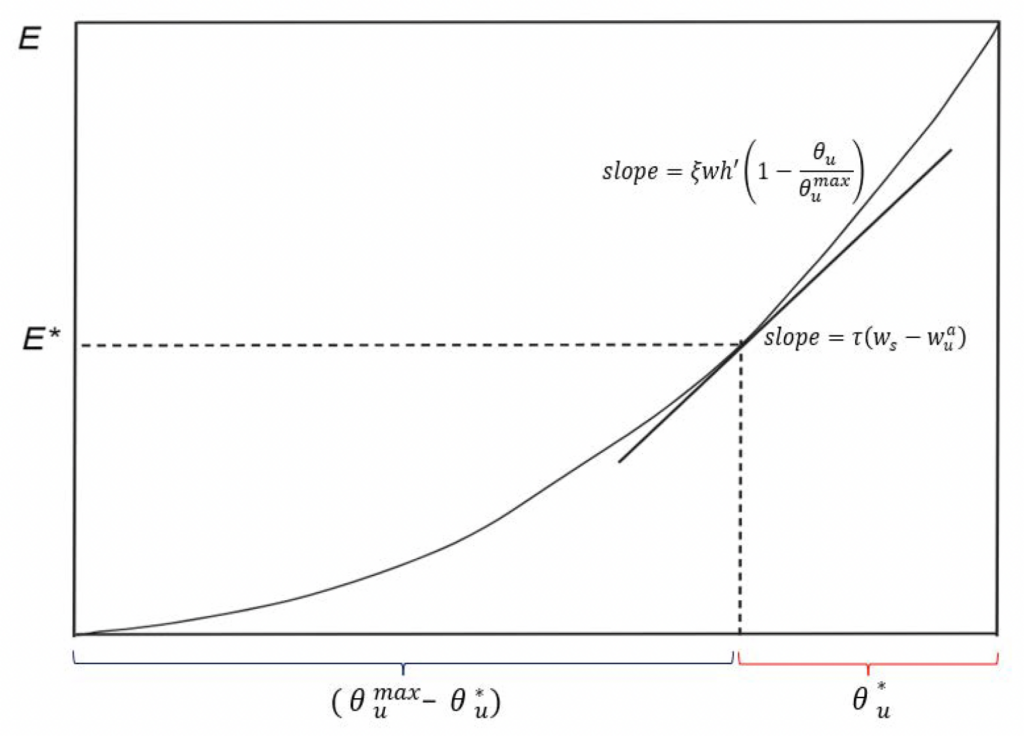
Figure 1 illustrates the optimal levels of enforcement $E^{\ast}$ and unauthorized immigration $\theta_{u}^{\ast}.$ The horizontal axis represents the pool of potential unauthorized immigrants $\theta_{u}^{\max},$ which is the amount of unauthorized immigration that would take place in the absence of any enforcement. These optimal levels are found when the slope $\xi wh^{\prime}\left( 1-\theta_{u}/\theta_{u}^{\max}\right)$ of the enforcement function $E\left( \cdot\right)$ equals the fiscal marginal cost of unauthorized immigration $\tau\left( w_{s}-w_{u}^{a}\right)$ . The horizontal axis is split into agents that are deterred from becoming unauthorized immigrants (either deported or dissuaded), to the left of the tangency point, and those who succeed in crossing into the host country, to the right of the tangency point.

The optimal level of unauthorized immigration is described by

(11) $\begin{equation*}\frac{\theta_{u}^{\ast}}{\theta_{u}^{\max}}\equiv\Upsilon=\left{\widetilde{\Upsilon}:\tau\left( w_{s}-w_{u}^{a}\right) =\xi wh^{\prime}\left( 1-\widetilde{\Upsilon}\right) \right} ,\end{equation*}$

where it can be shown that the optimal ratio $\Upsilon\equiv\frac{\theta{u}^{\ast}}{\theta{u}^{\max}}$ is (i) necessarily between $0$ and $1$ due to the properties of $h\left( \cdot\right)$ and (ii) increasing in $\frac{\xi w}{\tau\left( w_{s}-w_{u}^{a}\right) }.$ Hence, the optimal enforcement expenditure is given by

(12) $\begin{equation*}E^{\ast}=\xi w\theta_{u}^{\max}h^{\ast};\text{ for }h^{\ast}=h\left(1-\Upsilon\right) . \end{equation*}$

Figure 1. Optimal enforcement and unauthorized immigration

All else constant, $\theta_{u}^{\ast}$ and $E^{\ast}$ are proportional to the pool of potential migrants $\theta_{u}^{\max}$ .

4.2 Optimal Immigration in a Simpler Setting

A simpler version of the model that (i) ignores the enforcement cost (which can be obtained under the assumption that $\xi=0)$ and (ii) assumes that natives do not care about the family reunification motive (set $\gamma=0$ ) yields the conclusion that if immigration is justified (positive optimal immigration requires as a necessary condition that immigrants to have a high enough productivity level), then it would be exclusively of the skill-based type, while setting the other types of immigration to $0$ . This is because in this setting, skill-based immigrants improve the fiscal position of the country more than other types of immigrants (other immigrants might worsen the fiscal position depending on parameterization) while decreasing the availability of the common resource as much as other types of immigrants, thus the optimal policy is exclusively allowing some level of the skilled immigrants and zero of the other types. The full model considered in this paper helps to explain why countries have different immigration categories and also highlights the trade-offs of the different immigration choices.

4.3 An Analytic Solution

The comparative statics of the general model are intractable in the absence of more structure. In what follows, the model is analyzed under the assumption that the functions $u\left( \cdot\right),$ $v\left( \cdot\right)$ and $\widetilde{v}\left( \cdot\right)$ are all logarithmic (e.g. $u(x)=ln\left( x\right)$ ), in which case an analytic solution exists. Both Benhabib and Jovanovic (2012) and Guerreiro et al. (2020) also use logarithmic utility in their models.

In addition to being a popular choice in theoretical and applied work, there is another justification for assuming logarithmic utility: if the model is to produce a demand for immigration that is homogeneous of degree $0$ in all wages of the model, then $u\left( \cdot\right)$ ought to be logarithmic. ¹³^,¹⁴ The proof of this is in Appendix A.3.

At an interior solution, optimal transfers and immigration quotas, other than $\theta_{u}^{\ast}$ , are

(13) $\begin{equation*}b^{\ast}=\frac{\tau w_{s}}{\left( 1+\alpha\right) },\end{equation*}$

(14) $\begin{equation*}\theta_{F}^{\ast}=\frac{\gamma\left[ \frac{E^{\ast}}{\tau}+\left(w_{s}-w\right) +\left( w_{s}-w_{u}^{a}\right) \Upsilon\theta_{u}^{\max}\right] }{\left( w_{s}-w_{F}\right) \left( \alpha-\gamma\right) },\end{equation*}$

(15) $\begin{align*} \theta_{s}^{\ast} & =\frac{\left( 1+\Upsilon\theta_{u}^{\max}\right) \left[ w_{s}-w_{F}\left( 1+\gamma\right) \right] +\gamma\left[ w-\frac{E^{\ast}}{\tau}+\Upsilon\theta_{u}^{\max}w_{u}^{a}\right] }{\left( w_{s}-w_{F}\right) \left( \alpha-\gamma\right) } \\ & -\frac{\left( 1+\alpha\right) \left[ w-\frac{E^{\ast}}{\tau}+w_{u}^{a}\Upsilon\theta_{u}^{\max}\right] }{w_{s}\left( \alpha-\gamma\right) },\nonumber \end{align*}$

while the expressions for legal $\theta_{F}^{\ast}+\theta_{s}^{\ast}$ , and total immigration $\theta_{s}^{\ast}+\theta_{F}^{\ast}+\theta_{u}^{\ast}$ are given by

(16) $\begin{equation*} \left( \theta_{F}^{\ast}+\theta_{s}^{\ast}\right) = \frac{w_{s}\left(1+\Upsilon\theta_{u}^{\max}\right) \left(1+\gamma\right) - \left(1+\alpha\right) \left[\left(w-\frac{E^{\ast}}{\tau}\right) + w_{u}^{a}\Upsilon\theta_{u}^{\max}\right]}{w_{s}\left(\alpha-\gamma\right)}, \end{equation*}$

(17) $\begin{equation*} \left( \theta_{F}^{\ast} + \theta_{s}^{\ast} + \theta_{u}^{\ast} \right) = \frac{\left( 1+\gamma \right)}{\left( \alpha-\gamma \right)} + \frac{\left( 1+\alpha \right) \left[ \Upsilon\theta_{u}^{\max}\left( w_{s} - w_{u}^{a} \right) - w + \frac{E^{\ast}}{\tau} \right]}{w_{s}\left( \alpha-\gamma \right)}, \end{equation*}$

where $E^{\ast}$ is given by (12) and both $\Upsilon$ and $\theta_{u}^{\ast}$ are described by (11).

4.4 Comparative Statics

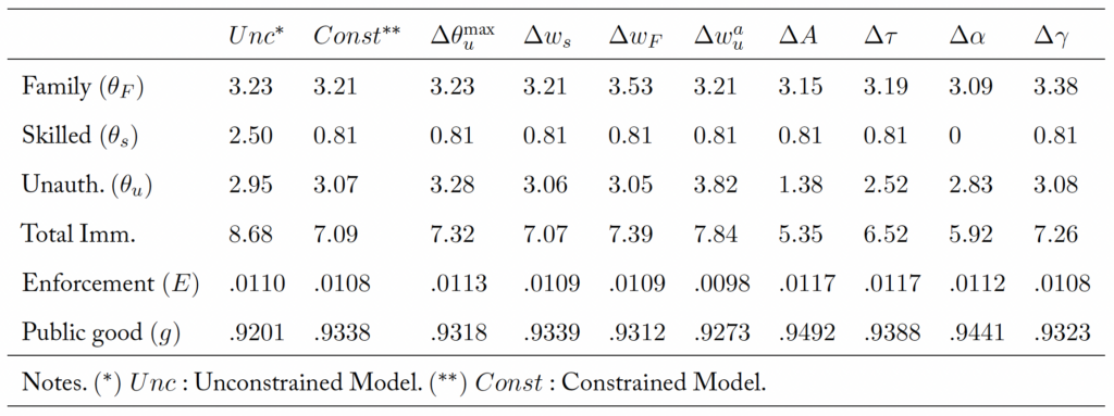
Table 1 summarizes the comparative statics for the model, with the particular derivations presented in Appendix B.

At an interior solution, the model predicts the following:

1. If the pool of unauthorized immigration $\theta_{u}^{\max}$ increases, the optimal response is to increase enforcement expenditure together with the equilibrium level of unauthorized immigration, as they are proportional to $\theta_{u}^{\max}$ by equations (11) and (12). Since the extra immigration decreases the utility cost of family-based immigration in condition (8), family-based immigration increases as a result. Skill-based immigration increases to mitigate the fiscal effects of immigration of the other two types.

2. A higher cost of enforcement $\xi$ leads to higher levels of unauthorized, family-based, and total immigration. The change in skill-based immigration is indeterminate.

3. Higher wages for skill-based immigrants $w_{s}$ enable higher enforcement expenditure, decreasing unauthorized immigration while increasing legal immigration.

4. Higher wages for unauthorized immigrants $w_{u}^{a}$ lead natives to spend less on enforcement and thus allow more unauthorized immigrants, while optimally decreasing family-based, legal, and total immigration.

5. Higher productivity of the family-based immigrants $w_{F}$ leads to unchanged legal immigration, but with a composition favoring a higher level of family-based immigrants over skill-based immigrants. Unauthorized immigration is unaffected.

Table 1. Comparative Statics

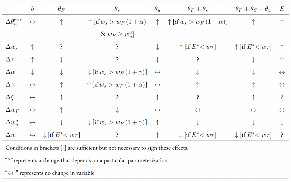
6. Higher productivity of the natives $w$ produces higher demand for unauthorized immigration and, depending on whether $E^{\ast}{\small <w\tau,}$ the demand for family-based immigration decreases. The effects on legal and total immigration are also negative when $E^{\ast}{\small <w\tau,}$ which is a condition easily met in reality (see next section).

7. A higher tax rate $\tau$ decreases unauthorized, family-based, and total immigration. Enforcement expenditures increase.

8. A bigger weight in the common resource parameter $\alpha$ lowers the demand for legal immigration (family + skill-based) while leaving unauthorized immigration unchanged.

9. A bigger weight in the reunification-motive parameter $\gamma$ increases demand for family-based immigration, where additional skilled-based immigration is used to ameliorate the induced fiscal pressures. Unauthorized immigration is unchanged.

5 Parameterization of the Model

The model is parameterized to represent the period 1994-2008, which is a time period that allows for several parameters to be obtained and is also the period used by Guerreiro et al. (2020). Table 2 presents the baseline parameterization.

Wages of natives are normalized at a level of $1$ . For the wages of family-based immigrants, Borjas and Friedberg (2009) report a $20\%$ wage gap between legal migrants and natives, which implies setting $w_{F}$ at a level of $80\%$ of natives’ wages ( $\frac{w_{F}}{w}=0.8$ ) and thus $w_{F}=0.8$ .

Regarding the wage gap between authorized and unauthorized immigrants, Rivera-Batiz (1999) and Kossoudji and Cobb-Clark (2002) estimate a wage gap of $7.5\%$ , while Barcellos (2010) reports a wage gap of $5\%$ . The gap is with respect to the observed wages $w_{u}$ of unauthorized immigrants. Using $\frac{w_{u}}{w_{F}}=\left( 1-gap\right),$ then $w_{u}$ is between $.74$ (gap $=7.5\%$ ) and $.76$ (gap $=5\%$ ). Thus $w_{u}$ is set at the average level of $0.75$ .

The model requires adjusted wages $w_{u}^{a},$ which could be estimated from Equation (3) but doing so is particularly complicated since it depends on (i) the degree to which unauthorized immigrants pay taxes $\lambda,$ and (ii) transfer savings $\eta,$ both of which are particularly complicated to estimate for a number of reasons.¹⁵ Instead, the paper proceeds by assuming that the savings in transfers would be approximately of the same magnitude as the loss in taxes, which implies $\eta=\tau\left( 1-\lambda\right) w_{u}$ and therefore $w_{u}^{a}$ $=w_{u}=0.75$ . The sensitivity analysis in Section 6 shows that the model is robust to alternative levels of $w_{u}^{a}$ , rendering the point moot. For a discussion of programs for which unauthorized immigrants do not qualify, see Kolker (2022) or Blau and Mackie (2017), and for a thorough discussion on static versus dynamic issues of fiscal impacts of immigrants, see Blau and Mackie (2017).

Table 2. Baseline Parameterization

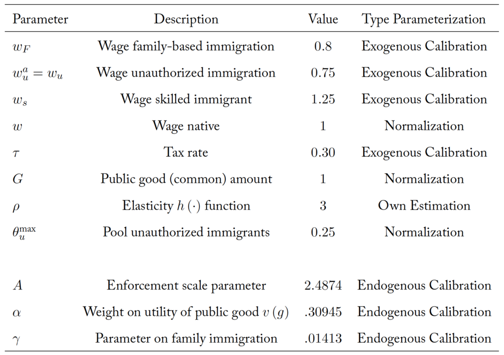
Chassamboulli and Peri (2015) estimate a $68\%$ wage premium for skilled labor over unskilled labor, using data from IPUMS USA for the years 2000-2010. Since the model’s unauthorized immigrants can be identified as unskilled, this suggests setting $\frac{w_{s}}{w_{u}}=1.68$ . This in turn implies that the skill-to-native-wage ratio is $\frac{w_{s}}{w} = \frac{w_{s}}{w_{u}} \cdot \frac{w_{u}}{w} = 1.68 \cdot 0.74 = 1.2432$ . The wage $w_{s}$ is set at $1.25$ .

The tax rate $\tau$ is set at a level of $30\%$ , as in Bohn and Lopez-Velasco (2018), and is revisited in the sensitivity section. The parameter $G$ (the amount of the common resource) is normalized at a level of 1 since its level does not affect immigration magnitudes.

For the enforcement sector, the production function $f\left( \cdot\right),$ linking the percentage of enforcement agents ( $\%$ natives) to the rate of enforcement, is given by $f\left( x\right) =A\left( x\right) ^{\frac{1}{\rho}}$ for $\rho>1$ and efficiency index $A>0$ . Appendix C shows that the associated expenditure function is given by $E\equiv\xi w\theta_{u}^{\max}\left( 1-\frac{\theta_{u}}{\theta_{u}^{\max}}\right) ^{\rho}$ , where in this case $h=\left( 1-\frac{\theta_{u}}{\theta_{u}^{\max}}\right) ^{\rho}$ and the previously defined constant $\xi$ is therefore given by $A^{-\rho}$ . Given these expressions, in an interior solution the optimal amount of unauthorized immigration in Equation (11) is

(18) $\begin{equation*}\theta_{u}^{\ast}=\theta_{u}^{^{{\max}}}\left[ 1-\left( \frac{\tau A^{\rho }\left( w{s}-w_{u}^{a}\right) }{w\rho}\right) ^{\frac{1}{\rho-1}}\right]. \end{equation*}$

The parameter $\rho$ is estimated econometrically. More specifically, Appendix C shows that it is possible to estimate a lower bound on it, found to be about $2.1$ . Since this number is a lower bound, the parameter is set to $3$ . This implies a production function in the enforcement sector given by $M_{D}=A\left( N_{E}\right) ^{\frac{1}{3}}\left( M_{u}^{\max}\right)^{\frac{2}{3}}$ where $N_{E}$ is the number of natives working in the enforcement sector; $M_{D}$ is the number of people who are apprehended and deported or dissuaded from migrating from the available pool $M_{u}^{\max}$ . This production function is reminiscent of a matching function in the context of matching models. Whether $\rho$ is $2.5$ or $4$ matters little for the conclusions, as the qualitative results are robust to this parameter (see sensitivity analysis).

The size of the pool of immigrants $\theta_{u}^{\max}$ is unobservable. A level of $25\%$ of the native population is used and this represents about 8 times the unauthorized quota allowed into the US for this period. Other numbers are considered in the sensitivity section, which shows that the level of this parameter is unimportant for the quantitative and qualitative effects of the parameterized model.

The remaining three parameters that jointly determine three moments in the data, those given by the immigration quotas as percentages of natives, are internally calibrated. The parameters are (i) $\alpha,$ which determines the importance of the common resource; (ii) $\gamma$ , which partially governs the strength of the family-based immigration motive; and (iii) the parameter $A$ from the production function in the enforcement sector (where $\xi=A^{-\rho}%)$ . The particular calibration strategy is explained after documenting the immigration calibration targets.

According to the Department of Homeland Security,¹⁶ the total number of foreigners obtaining permanent resident permits for the period 1994 to 2008 via family-based immigration (i.e. the sum of immediate relatives of US citizens + family-sponsored preferences) was $8,841,754$ , while there were $2,043,391$ foreigners who obtained one due to employment-based preferences. Regarding the unauthorized population, the paper uses the estimates in Warren and Warren (2013) for the years 1994 to 2005, while data starting in 2005 onward is available from the Department of Homeland Security. The change in the stock of new unauthorized immigrants for this period is computed at a level of $7,034,899$ . Taking into account a legalization rate of about $0.7\%$ per year (as estimated in Chassamboulli and Peri (2015) for the period 2009-2010), the number of family-based immigrants is corrected by a factor $(1-.007)^{14}%=0.90634$ to be $8,841,754\ast.90634=$ $8,114,777$ , and the number of unauthorized immigrants that stayed during this period is therefore $7,034,899/.90634=7,761,876$ . The average population in the US during that period (net of the foreign-born population in order to compute “natives”) was $252,482,693$ , which yields immigration targets of $\theta_{F}=3.21\%,$ $\theta_{s}=0.81\%$ and $\theta_{u}=3.07\%$ , while total immigration as percentage of natives is their sum, $7.09\%$ , which represents almost $18$ million immigrants for the period or about $1,280,000$ per year (including unauthorized immigrants). More specifically, there were about $780,000$ permits given annually to family-based and skill-based immigrants, while roughly $500,000$ new unauthorized immigrants arrived each year.

Given $\theta_{u}^{\max}$ and $\rho,$ the parameter $A$ can be identified from expression (18). Solving for $A$ yields the calibrating expression of

$\widehat{A} = \left[ \frac{w\rho}{\tau\left( w_{s} - w_{u}^{a} \right)} \right]^{\frac{1}{\rho}} \left( 1 - \frac{\theta_{u}^{\ast}}{\theta_{u}^{\max}} \right)^{1 - \frac{1}{\rho}}.$

Substituting the other parameters and the target $\theta_{u}^{\ast}=.0307$ yields $\widehat{A}=2.4874.$

The last 2 parameters to calibrate are $\alpha$ and $\gamma.$ These two parameters can be jointly determined from expressions (14) and (15), as they form a system of two equations in two unknowns ( $\alpha,\gamma$ ) which yields calibrating expressions given by

(19) $\begin{align*} \widehat{\alpha} & =\frac{\tau w_{s}\left( 1+ \sum \theta_{i}^{\ast}\right) }{\tau\left( w+ \sum w_{i}\theta_{i}^{\ast}\right) -E^{\ast}}-1, \\ \widehat{\gamma} & =\widehat{\alpha}\left( \frac{\left( w_{s}-w_{F}\right) \theta_{F}^{\ast}}{\left( w_{s}-w_{F}\right) \theta_{F}^{\ast}+\left( \frac{E^{\ast}}{\tau}+w_{s}-w\right) +\left( w_{s}-w_{u}^{a}\right) \theta_{u}^{\ast}}\right) . \end{align*}$

Replacing the other parameters and the three calibrating targets, the above expressions yield $\widehat{\alpha}=.30945$ and $\widehat{\gamma}=.01413.$ The structure of the model yields calibrating expressions to $A,$ $\alpha,$ and $\gamma$ that exactly hit the three targets given by the immigration quotas.

5.1 Experiments with the Parameterized Model

This section documents the responses of optimal immigration in the calibrated model to a $5\%$ change in each of the parameters.

For this and the remaining experiments, there is an additional parameter that needs to be considered: the supply of skill-based immigrants. It could be assumed that the level observed empirically is a supply-side constraint, since the US competes on skilled immigration with other developed economies.
However, the fact that H1B visas are typically exhausted suggests evidence to the contrary. The paper takes a pragmatic position and chooses a supply level that is higher than what is observed. Specifically, an initial level of .025 is assumed for this parameter ( $2.5\%$ of natives during a 14-year period, which represents a supply of 450,000 skill-based immigrants per year versus an historical average of 145,000 permits for this period). However, other numbers yield similar conclusions, since for the majority of changes considered, this parameter does not play a significant role—as shown in the sensitivity analysis in Section 6. The findings are as follows.

A $5\%$ increase in the pool of unauthorized immigrants $\theta_{u}^{^{_{\max}}%}$ yields an optimal response of higher enforcement spending, but allows more unauthorized immigration than before ( $3.22\%$ instead of $3.07\%$ ), with skill-based immigration increasing significantly from $.81\%$ to $1.55\%$ of natives while family-based immigration is essentially unchanged ( $3.24\%$ vs $3.21\%$ ).

An increase of $5\%$ in the wages of skill-based immigrants $w_{s}$ leads skill-based immigration to hit the supply-side limit of $2.5\%$ and prompts a reduction in unauthorized immigration from $3.07\%$ to $2.90\%$ . The extra resources from skilled-based immigration are used in part towards enforcement expenditures. Family-based immigration is mostly unaffected ( $3.24\%$ as opposed to $3.21\%$ ).

A $5\%$ increase in the wages of family-based immigrants $w_{F}$ does not affect unauthorized, legal, or total immigration; it only results in a one-to-one crowding-out of skill-based immigrants (from $0.81\%$ to $0.50\%$ ) in favor of family-based immigrants (now $3.52\%$ ).

A $5\%$ increase in the wages of unauthorized immigrants $w_{u}^{a}$ diminishes the importance of enforcement and thus unauthorized immigration increases to $3.87\%$ . Skill-based immigration is set to 0. Total and family-based immigration remain practically unchanged at $7.07\%$ and $3.20\%$ , respectively.

When the model considers an improvement of $5\%$ in the technology of enforcement $A$ , the optimal response is to significantly decrease unauthorized immigration to $1.40\%$ (from $3.07\%$ ), leaving family-based immigration unchanged while also decreasing skill-based immigration to $0.57\%$ . Total immigration is reduced significantly to $5.12\%$ of natives.

An increase in the tax rate $\tau$ of $5\%$ (from $30\%$ to $31.5\%$ ) makes overall immigration less desirable but unauthorized immigration decreases the most, from $3.07\%$ to $2.53\%$ . Skill-based immigration likewise decreases from $0.81$ to $0.73\%$ , while family-based is almost unaffected at $3.19\%$ .

When the parameter $\alpha$ increases $5\%$ , natives care more about the non-economic externalities imposed by immigrants, and as a result the demand for immigration decreases: family-based immigration reduces to $3.09\%$ , unauthorized immigration decreases to $2.83\%$ , and skill-based immigration is set to 0.

Finally, when the parameter $\gamma$ is increased $5\%$ , family-based and skill-based immigration increase to 3.38 and 0.90 respectively, leaving unauthorized immigration unchanged. In this case, additional skill-based immigration helps to absorb the fiscal effects of additional family-based immigration.

Table 3. Effects of a 5% change in parameters

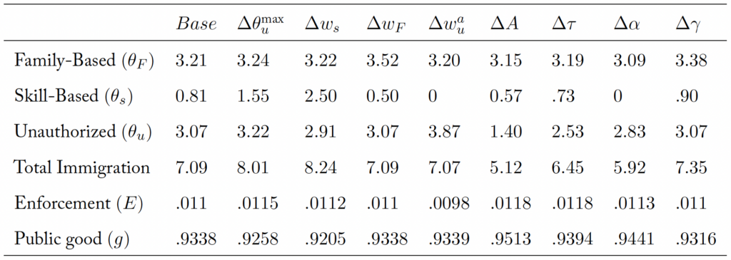
One of the messages from these experiments is that skill-based immigration has a “shock-absorber” role. A larger number of skill-based immigrants are allowed whenever (i) the pool of unauthorized immigrants increases, (ii) the wages of family-based or unauthorized immigrants decrease, (iii) technology in the enforcement sector worsens, or (iv) the family-reunification motive becomes more important. Skill-based immigration increases in order to help pay for more expensive enforcement and to minimize the fiscal effects on the transfer.

Another message from these experiments is that in the optimal policy and in contrast with the other categories, family-based immigration is not responsive to most parameters, other than with respect to the wage of said immigrants.

5.2 Calibration under Suboptimal Immigration Flows

The strategy employed to calibrate the model in the previous section assumes that the observed behavior is optimal. Judging by previous attempts at immigration reform, which are more thoroughly discussed in the next section, it is also possible that the observed magnitudes are suboptimal, reflecting (for example) some exogenous political constraint.

To study the implications of this scenario, the model is parameterized under the assumption that optimal skill-based immigration is higher than the observed flows, as H1B visas are consistently exhausted. In this case, the optimal choice of skill-based immigration would be unobservable and as a result, the observed unauthorized and family-based magnitudes would be a constrained maxima in the presence of an exogenous constraint on the maximum level of skill-based immigration.

Table 4. Effects of a 5% change in parameters in the constrained model

Let the optimal immigration quotas that yield the constrained maxima be defined by $\theta_{s}^{c},$ $\theta_{F}^{c}$ and $\theta_{u}^{c}$ . The observed magnitudes would identify such levels and therefore $\theta_{s}%^{c}=.81,$ $\theta_{F}^{c}=3.21,\theta_{u}^{c}=3.07.$ To calibrate the model in this environment, the optimal unconstrained level of skill-based immigration $\theta_{s}^{\ast}$ has to be specified (assumed) since such magnitude could not be backed from observables. Absent this piece of information, there would be a whole family of parameterizations for $\left( A,\alpha,\gamma\right)$ that yield the constrained levels.

The level for the optimal unconstrained level of skilled immigration is assumed to be $\theta_{s}%^{\ast}=2.5\%$ (other numbers work as well, provided they are higher than $0.81\%$ ), but this section is mostly illustrative. The calibration then would require choosing parameters that yield constrained magnitudes $\theta_{s}%^{c}=.81\%,$ $\theta_{F}^{c}=3.21\%,$ $\theta_{u}^{c}=3.07\%$ , while also producing an unconstrained level of skilled-based immigration of $\theta {s}^{\ast}=2.5\%$ . The first-order conditions of the constrained system, together with equation (15) can be used to obtain alternative calibrating expressions, which yield $\widehat{A}{c}=2.4966$ , $\widehat{\alpha}{c}=0.303164$ and $\widehat{\gamma}{c}=0.013952$ . The details on the alternative calibration procedure are shown in Appendix D.

Table 4 presents the comparative statics of the constrained model. It is instructive first to compare the first two columns, which present the (implied) unconstrained model under the new parameterization, alongside the constrained version of the model. Family-based immigration would essentially remain unchanged ( $3.23\%$ instead of $3.21\%$ ), but unauthorized immigration is higher in the constrained version ( $3.07\%$ ) than it would be if skilled-based immigration were larger ( $2.95\%$ ). Some of the fiscal boon due to the higher skill-based immigration would be spent on a higher level of enforcement, as well as higher transfers.

The main difference with respect to the results of the unconstrained model of the previous section is that in the current model, skill-based immigration does not decrease as a result of 1) higher wages of unauthorized immigrants, 2) higher wages of family-based immigrants, 3) better enforcement technology, or 4) a higher tax rate. Both family-based and unauthorized immigration have similar comparative statics to the unconstrained version, with just small differences in magnitudes.

5.3 On the Demand for US Immigration Reform

This section comments on the demand for US immigration reform through the lens of the model. This is not to be interpreted as responses to short-run fluctuations in immigration flows, but rather as permanent changes in the immigration framework that governs immigration flows. Some examples of these changes include the 1965 Immigration and Nationality Act, which created most of the modern framework of US immigration policy, and the Immigration Act of 1990, which sets specific limits for the different categories and preferences on immigrants, and which also created (among other things) the H1B visa category.

Two salient facts stand out during the period of analysis, both of which have implications for the demand for immigration reform: 1) the increase of the skill premium, and 2) the significant increases in unauthorized immigration flows to the US.

With respect to the evolution of the skill premium, Acemoglu and Autor (2012) report an increase of almost $10\%$ in the hourly wages of college graduates vs. those of high school graduates, for the 1994-2008 period. The model predicts that higher wages for skilled-based immigrant lead to a higher demand for them, roughly unchanged family-based immigration, and decreased demand for unauthorized immigration.

In order to capture the above effect in the model, we must ascertain the skill composition of natives. Bohn and Lopez-Velasco (2018) compute the share of the population 25 years and older with a bachelor’s degree or higher education, and they find this number to be $27.7\%$ in the 2000-2009 decade and $22.8\%$ in the 1990-1999 decade. The average for this period is almost $25\%$ , which is used in the calculations here. Given these numbers, a $10\%$ increase in the skill premium represents a $6.67\%$ increase in the wages of skill-based immigrants relative to those of natives.¹⁷

In the 1980s, there was an average of about 225,000 new unauthorized immigrants per year, according to the panel of scientists at the National Research Council (Smith and Edmonston (1997)). These flows accelerated significantly in the 1990s and 2000s. The current paper implies a flow of roughly 500,000 new unauthorized immigrants per year for the period 1994-2008.¹⁸ This increase in unauthorized immigration took place even in the presence of higher border patrol expenditure, which steadily increased from $.0055\%$ of GDP in 1994 to $.0153\%$ of GDP in 2008.¹⁹ These numbers suggest that the pool of potential unauthorized immigrants increased during this period, as the model predicts higher enforcement and higher unauthorized immigration in response.

Other factors also suggest a bigger pool of potential unauthorized immigrants. Changes in income per capita, unemployment rates, and the population growth rates of the US and the main sending countries are consistent with this inference. The sending countries are mostly in Latin America and the Caribbean, which accounted for $87\%$ of all unauthorized immigrants in the US in the year 2000.²⁰ During this period, GDP per capita in constant PPP dollars increased by $30.4\%$ in the US, compared to $26.5\%$ for the sending countries. Second, although the unemployment rate in the US was slightly higher than the average unemployment rate in Latin America in the early 1990s ( $6.9\%$ vs. $6.15\%$ in 1993, according to World Development Indicators), it was lower in the US in every year during this period, with an average gap of 3 percentage points. Third, population growth in the sending countries for the 15-64 age group was $31.3\%$ , while the same age group in the US grew by $18.4\%$ .

One way to parsimoniously estimate the growth of the pool of unauthorized immigrants is by using the difference in population growth rates between the sending countries and the US population, which is almost $13\%$ . In what follows, both changes (an increase in $\Delta w_{s}$ by $6.67\%$ and an increase in $\Delta\theta_{u}^{\max}$ by $13\%$ ) are fed into the model, first one at a time and then both at the same time, in the original and the alternative calibrations. Table 5 presents these results.

Both shocks produce higher demand for skill-based immigration, to the point where the supply-side limit becomes binding. The demand for family-based immigration increases very little from both shocks (to $3.27\%$ of natives as opposed to $3.21\%$ ), while unauthorized immigration would decrease to $2.90\%$ as a result of the increase in $w_{s}$ , but increases to $3.49\%$ of natives due to the higher level of $\theta_{u}^{\max}$ . Adding both shocks together would ultimately increase it to $3.43\%$ of natives as the effect on $\theta_{u}^{\max}$ dominates the effect on $w_{s}$ .

Table 5. Effects on Immigration Magnitudes if $\Delta w_{s} =6.67\%$ and $\Delta\theta_{u}^{\max}=13\%$

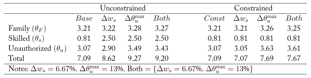
If the initial flow of unauthorized immigration was about 225,000/year in the 1980s (the 1970s had similar flows according to Edmonston and Passel (1994)), then the unconstrained model would predict an increase in the flows of unauthorized immigration from $3.07\%$ to $3.43\%$ of natives, which represents an average flow of about 250,000 unauthorized immigrants per year.

In the case of the constrained model, skill-based immigration cannot respond as a “shock-absorber” (it can decrease but not increase beyond the maximum number of permits, which is fixed) and thus unauthorized immigration increases more than in the unconstrained case. Unauthorized immigration would increase to $3.61\%$ of natives, about 265,000 new unauthorized immigrants per year, representing about $53\%$ of the observed level. This exercise is just suggestive since the number of potential unauthorized immigrants is not directly observable, and since its change might have been much bigger than the estimate given by the difference in population growth rates.

In light of the analysis above, the constrained model could address the question “what could explain what happened during this period?” since there can be deviations from optimality due (for example) to political constraints, while the unconstrained model instead addresses “what immigration policy would the native population have preferred in response to these changes?”

With regard to family-based immigration, the unconstrained model suggests a small increase for this period, one that can be accommodated within current policy. In particular, family-based immigration of immediate relatives is not bounded, while permits for other family-based preferences are indeed subject to the annual caps, which results in waiting time for many family-based cases. The insight from the model is that family-based immigration changes very little in response to the above forces, and this can be accommodated by the current system emphasizing family reunification.

In the case of skill-based immigration, the model suggests significant increases to reach optimal levels. The number of permits allocated to employment-based immigration has not changed since the 1990s, with a maximum annual cap of 140,000. However, there were some changes in the H1B visa program that allowed for additional skill-based immigration. Initially, the program allocated a maximum of 65,000 permits annually. Then there were temporary expansions in the cap, with 115,000 permits allocated for years 1999 and 2000, then a cap of 195,000 in years 2001–2003. This number reverted to 65,000 afterwards, but starting in 2006 there were an extra 20,000 visas available for foreigners who graduated from US universities with master’s or doctorate degrees and thus were not subject to the cap (see American Immigration Council (2023)). While the H1B visa is for temporary immigration, this program is recognized as one of dual intent, which means that foreigners with this visa have the option to apply for permanent residence.²¹

The efforts to pass major immigration reforms during the analyzed period are also informative. Kandel, Wilson, and Donovan (2022) discuss the characteristics of the last three attempts at comprehensive immigration reform in the US. In 2006 there was the “Comprehensive Immigration Reform Act of 2006,” then in 2007 there was “A bill to provide for comprehensive immigration reform and for other purposes,” and finallly in 2013 there was the “Border Security, Economic Opportunity, and Immigration Modernization Act.” All three proposals (i) do not modify the current system that emphasizes family-reunification of immediate relatives, (ii) provide more funding and new tools towards enforcement, (iii) either eliminate the diversity visa program or reduce it considerably, and finally and perhaps most importantly, (iv) add significantly more skill-based immigration permits.²² Taken together, the proposed changes are largely consistent with the immigration policies predicted by the model: no change to family-based immigration, significantly more permits for skill-based immigration and adequate enforcement expenditure that depends on the supply of potential unauthorized immigrants.

6 Sensitivity Analysis

For robustness, this section documents the effects of alternative parameters on the quantified effects discussed previously for both calibrations of the model. Specifically, the sensitivity analysis considers alternative values for $w_{u}^{a}$ of 0.6 and 0.9, alternative values of the parameter $\rho$ of 2.5 and 4, alternative tax rates $\tau$ of $20\%$ and $40\%$ , as well as alternative values of the unauthorized immigration pool $\theta_{u}^{\max}$ of $10\%$ and $50\%$ of the native population. Overall, both the qualitative and quantitative effects are very similar to the main parameterizations considered above, and for simplicity they are not discussed in more detail. Results are presented in Table 6 for the unconstrained version and Table 7 for the constrained version.

Table 6. Effects of a 5% change in parameters in the unconstrained model

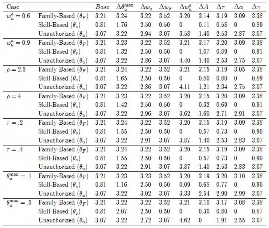
Table 7. Effects of a 5% change in parameters in the constrained model

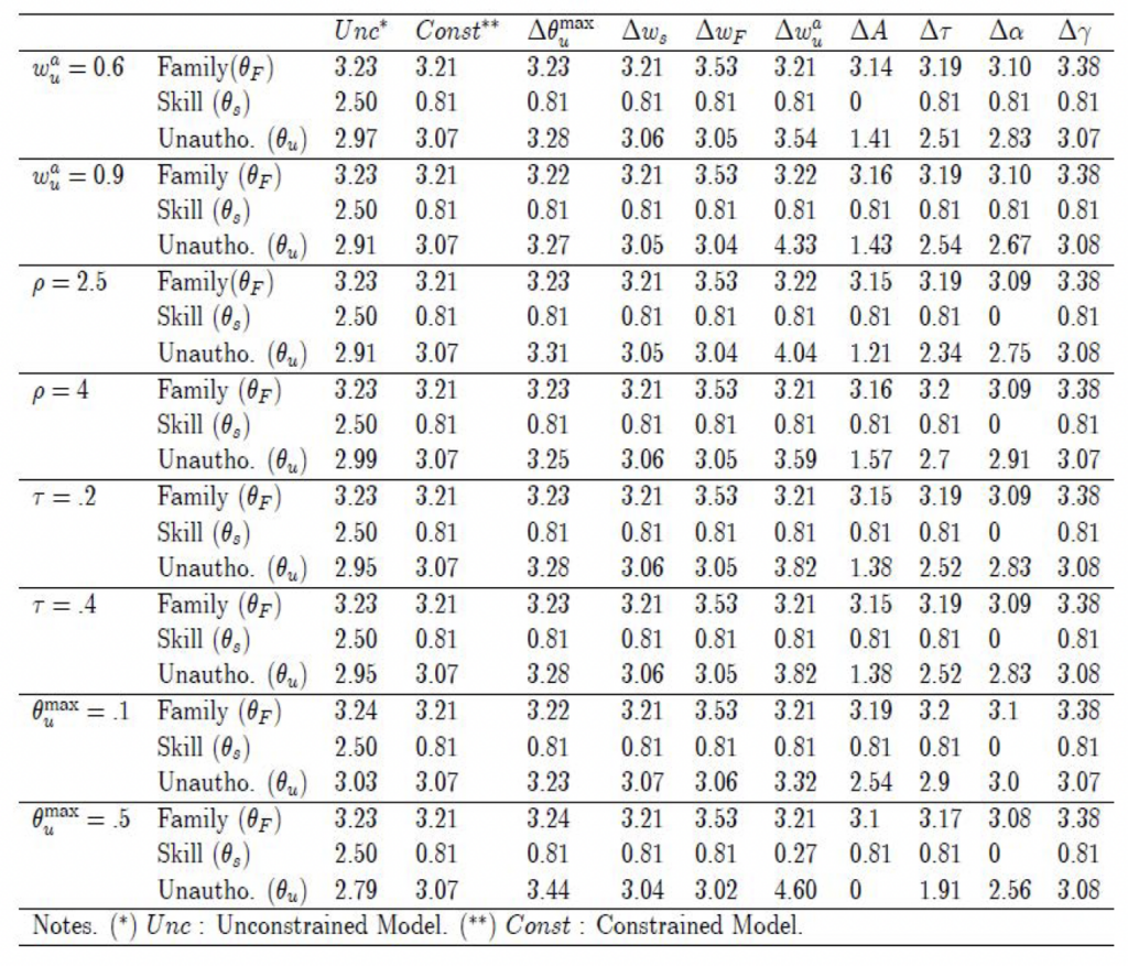
7 Some Policy Implications and Considerations Beyond the Model

Regarding the current inflow of unauthorized immigrants, the model makes the (perhaps obvious) point that not enforcing the border invites higher levels of unauthorized immigration and that enforcement is a necessary component of immigration policy. At the current level of abstraction, the model does not consider alternative tools like a guest worker program for low-skilled immigrants. In reality, a guest worker program could dissuade some would-be unauthorized immigrants by convincing them to migrate legally (and in a temporary way). This has the potential to represent a Pareto improvement for both immigrants (who would have more certainty about crossing without having to pay very high economic and human costs) and natives (who could spend less on enforcement and have more control over who specifically is crossing the border and for how long).²³

To address the case of family-based immigration, we first need to discuss the mapping of the model onto observed quotas. Family-based immigration is subdivided into i) “immediate relatives” that include spouses, minor children (under 21), and parents of American citizens, and ii) “family-sponsored preferences,” which includes unmarried or married adult children of American citizens, spouses or children of lawful permanent residents, and brothers and sisters of American citizens.

There is no limit on the number of visas available to ”immediate relatives,” which reflects the very high valuation placed on the nuclear family (at least in terms of spouses and young children). Their waiting time is mostly determined by the time it takes cases to be processed. But the family-sponsored preferences category follows more complicated rules that results in backlogs— some lasting decades.

Family-sponsored preferences are awarded a minimum of 226,000 permits a year, with the maximum determined by the difference between 480,000 and the number of permits awarded to immediate relatives.²⁴ In addition, no country can be allocated (between employment and family-based) more than $7\%$ of the total visas in a given year. The backlog is therefore a result of a rationing mechanism for the number of family-based immigrants similar to what the paper considers, as it assumes that the planner chooses the number of permits (thus demand-determined) from a bigger supply of immigrants who would like to come to the US.²⁵

The model also suggests that under the optimal policy, family-based immigration is not very responsive to most forces, other than to these immigrants’ fiscal contributions. However, extant data (see OECD (2017)) on economic outcomes of family-based immigrants is very limited, and data on the rate of service utilization is also hard to come by. At the very least, the paper suggests keeping track of outcomes by immigration permit type.

The forces analyzed for the period 1994−2008 predict a higher demand for skilled-based immigration, which is likely to be part of future proposals. The paper suggests that any reform could also include shock-absorbing features, which is perhaps even more important in light of the fact that immigration of immediate relatives is not limited in the US.

Finally, the insights from the model can also be used to think about immediate relatives. Permits for spouses and minor children are probably easy to justify as family reunification. But that is not so clear in the case of parents of American citizens. Economically, older adults are expected to contribute less/cost more to the welfare state (although they could help with non-market activities at home), but this calls for further discussion. An alternative for this type of immigration would also be some sort of longer-term temporary permit (lasting perhaps a few years), as opposed to the current system that emphasizes permanent immigration.

8 Conclusions

This paper studies optimal immigration in a model where agents receive a universal fiscal transfer financed by income taxes, there are congestion externalities of a public good, and border enforcement is costly. Welfare depends on (i) the transfer, (ii) the level of family-based immigration in the country, and (iii) a public good subject to congestion. This welfare function captures in a simple way a more complicated political environment where agents differ in their preferences over each of these issues, as in probabilistic voting models.

There are three types of immigrants: those with family ties to natives, those available for their skill (identified with employment-based immigration), and those who are able to migrate without permission (unauthorized), and each type has different productivity. Immigrants can increase or decrease the size of the fiscal transfer depending on whether their productivity is higher than that of natives, and all agents affect the availability of the public good. The optimal policy specifies quotas for each immigration type, the optimal enforcement level, as well as an optimal response to different long-run forces.

The paper obtains three conditions that jointly characterize the optimal policy. The first condition balances family-based with skill-based immigration. Family-based immigration provides direct utility for (some) natives but does not improve the fiscal position of the country as much (and depending on parameterization, it can deteriorate it) compared to skill-based agents. The second condition balances the effects on transfers against the congestion externalities imposed on natives. The last condition equalizes the fiscal opportunity cost of unauthorized immigration, relative to skill-based immigrants, to the marginal cost of enforcement. These new conditions in the literature jointly determine the optimal policy.

The paper calibrates this model in an attempt to quantify the response of the optimal policies, using the 1994-2008 period as reference. The experiments reveal several guiding principles. First, skill-based immigration is used as a ”shock-absorber,” as increasing it alleviates the negative fiscal impact of lower productivity of family-based immigrants or unauthorized immigrants, as well as responding to a bigger supply of unauthorized immigrants. Second, optimal family-based immigration is not responsive with respect to most parameters, other than with respect to family-based immigrants’ own productivity level and with respect to the preference parameter for family-based immigration. Finally, whenever there is an increase in the pool of potential unauthorized immigrants, the optimal policy is to increase enforcement expenditure while at the same time allowing more unauthorized immigrants.

There are two particular forces that stand out during the analyzed period: (i) the increase in the skill premium, and (ii) a very large increase in unauthorized immigration relative to previous decades. This could be consistent with a bigger supply of unauthorized immigration, as the observed increase took place in spite of higher enforcement expenditure.

The parameterized model suggests that both forces would lead to higher demand for skill-based immigration, with unchanged family-based immigration and higher unauthorized immigration, since the increase in the supply of unauthorized immigration dominates the decrease due to the higher skill premium, while both effects increase enforcement expenditure. This is to some extent consistent with what is observed in reality, as immigration changes had to do with increases in the H1B visa and higher enforcement budget while not affecting the family-based system. But in particular, it is consistent with the proposals for comprehensive immigration reform presented in the US in 2006, 2007 and 2012 which left the family-reunification system practically intact, gave more tools and budget for enforcement, and in particular devoted more permits to employment-based immigration.

Finally, the paper also presents an alternative calibration where the observed immigration flows are to be interpreted as suboptimal, since reform proposals at the time could reflect a desire for a higher level of skill-based immigration. The conclusions from this model are similar and show the robustness of the results of family-based immigration responding only to their productivity, as well as allowing more unauthorized immigration than when skill-based immigration can be adjusted.

While no model can reflect all of the important issues regarding immigration, the current model could be enriched by considering other issues which the literature has identified, including for example the role of networks and chain immigration. These issues are left for future research.

Appendix A Model Derivations

A.1 Optimality Conditions

The Lagrangian is given by

$\underset{b,\theta_{F},\theta_{s},\theta_{u},g}{\mathcal{L}} = u\left( b\right) + \alpha v\left( g\right) + \gamma \widetilde{v}\left( \theta_{F} \right)$

$+\mu_{1}\left[ \tau\left( w_{F}\theta_{F}+w_{s}\theta_{s}+w+w_{u}^{a}\theta_{u}\right) - b\left( 1+\theta_{F}+\theta_{s}+\theta_{u}\right) - \xi w\theta_{u}^{\max}h\left( 1-\frac{\theta_{u}}{\theta_{u}^{\max}}\right) \right]$

$+\mu_{2}\left[ G-g\left( 1+\theta_{F}+\theta_{s}+\theta_{u}\right)\right]$

with first-order conditions given by

(20) $\begin{equation*} \begin{aligned} b &: u^{\prime}(b) = \mu_{1}(1 + \theta_{F} + \theta_{s} + \theta_{u}) \\ g &: \alpha v^{\prime}(g) = \mu_{2}(1 + \theta_{F} + \theta_{s} + \theta_{u}) \\ \theta_{s} &: \mu_{1}[\tau w_{s} - b] = \mu_{2}g \\ \theta_{F} &: \gamma\widetilde{v}^{\prime}(\theta_{F}) + \mu_{1}[\tau w_{F} - b] = \mu_{2}g \\ \theta_{u} &: \mu_{1}[\tau w_{u}^{a} - b + \xi wh^{\prime}(1 - \theta_{u}/\theta_{u}^{\max})] = \mu_{2}g \\ \mu_{1} &: \tau(w_{F}\theta_{F} + w_{s}\theta_{s} + w + w_{u}^{a}\theta_{u}) = b(1 + \theta_{F} + \theta_{s} + \theta_{u}) + \xi w\theta_{u}^{\max}h(1 - \theta_{u}/\theta_{u}^{\max}) \\ \mu_{2} &: G = g(1 + \theta_{F} + \theta_{s} + \theta_{u}) \end{aligned} \end{equation*}$

Using the first-order conditions for $(b)$ and for $(g)$ , one obtains the Lagrange multipliers

$\begin{align*} \mu_{1} &= \frac{u^{\prime}(b)}{(1 + \theta_{F} + \theta_{s} + \theta_{u})} > 0, \\ \mu_{2} &= \frac{\alpha v^{\prime}(g)}{(1 + \theta_{F} + \theta_{s} + \theta_{u})} > 0, \end{align*}$

Hence, $\frac{\mu_{2}}{\mu_{1}}$ is given by

$\frac{\mu_{2}}{\mu_{1}} = \frac{\alpha v^{\prime}(g)}{u^{\prime}(b)}.$

From foc[ $\theta_{s}$ ] one can write $\left[ \tau w_{s}-b\right] =\frac{g\mu_{2}}{\mu_{1}}$ and from foc[ $\theta_{F}$ ] one can write $\frac{g\mu_{2}}{\mu_{1}}=\frac{\gamma\widetilde{v}^{\prime}\left( \theta_{F}\right) }{\mu_{1}}+\left[ \tau w_{F}-b\right] .$ Getting rid of $\frac{\mu_{2}g}{\mu_{1}}$ yields $\left[ \tau w_{s}-b\right] =\frac{\gamma\widetilde{v}^{\prime}\left( \theta_{F}\right) }{\mu_{1}}+\left[ \tau w_{F}-b\right].$ Then, canceling $b$ yields a condition that equates the marginal benefit of family reunification with its fiscal opportunity cost $\tau\left(w_{s}-w_{F}\right) =\frac{\gamma\widetilde{v}^{\prime}\left( \theta {F}\right) }{\mu{1}}.$ The equation can be rewritten by getting rid of $\mu_{1}$ as

$u^{\prime}(b) \frac{\tau(w_{s} - w_{F})}{(1 + \theta_{F} + \theta_{s} + \theta_{u})} = \gamma\widetilde{v}^{\prime}(\theta_{F}).$

which is Equation (8) in the text.

From the first-order conditions for $\theta_{s}$ and $\theta_{u}$ one can eliminate $\frac{\mu_{2}}{\mu_{1}}g\$ and obtain Equation (10)

$\tau\left( w_{s} - w_{u}^{a} \right) = \xi wh^{\prime}\left( 1 - \frac{\theta_{u}}{\theta_{u}^{\max}} \right).$

Replacing the multipliers from foc[ $g$ ] and from foc[ $b$ ] into foc[ $\theta_{s}$ ], one obtains

$\frac{u^{\prime}\left( b\right) }{\alpha v^{\prime}\left( g\right) }=\frac{g}{\left[ \tau w_{s}-b\right] },$

which is Equation (9) in the text.

A.2 The Analytic Solution

Assuming that $u\left( b\right) =\ln b;$ $\widetilde{v}\left( \theta {F}\right) =\ln\theta{F}$ and $v\left( g\right) =\ln g,$ the system of equations (5), (6), (10), (8), and (9) in the unknowns $b,$ $\theta_{F},$ $\theta_{s},$ $\theta_{u}$ and $g$ is given by

(21) $\begin{equation*}\frac{1}{b}\frac{\tau\left( w_{s}-w_{F}\right) }{\left( 1+\theta_{F}+\theta_{s}+\theta_{u}\right) }=\frac{\gamma}{\theta_{F}}\end{equation*}$

(22) $\begin{equation*}\tau\left( w_{s}-w_{u}^{a}\right) =\xi wh^{\prime}\left( 1-\frac{\theta{u}}{\theta{u}^{\max}}\right) \end{equation*}$

(23) $\begin{equation*}\frac{g}{\left[ \tau w_{s}-b\right] }=\frac{g}{\alpha b}\end{equation*}$

(24) $\begin{equation*}\tau\left( w_{F}\theta_{F}+w_{s}\theta_{s}+w+w_{u}^{a}\theta_{u}\right)=b\left( 1+\theta_{F}+\theta_{s}+\theta_{u}\right) +\xi w\theta_{u}^{\max}h\end{equation*}$

(25) $\begin{equation*}g\left( 1+\theta_{F}+\theta_{s}+\theta_{u}\right) =G\end{equation*}$

For simplicity of notation, equilibrium levels, which in turn are the solution to the above system, are denoted by $(^{\ast})$ .

The second equation in the above system (Equation (22)) yields an implicit solution to $\theta_{u}^{\ast}$ which is independent of the other equations and is precisely condition (10) in the text.

Equation (23) can be solved for $b^{\ast}$ and yields expression (13) in the text, given by

$b^{\ast}=\frac{\tau w_{s}}{\left( 1+\alpha\right) }.$

Inserting the solutions to $\theta_{u}^{\ast}$ and $b^{\ast}$ above into Equations (21) and (24) yields the solution to $\theta_{F}^{\ast}$ and $\theta_{s}^{\ast}$ , which is now shown.

First, $\theta_{F}^{\ast}$ is obtained. From (21), the term $\left( 1+\theta_{F}+\theta_{s}+\theta_{u}\right)$ can be written as $\frac{\tau\left( w_{s}-w_{F}\right) \theta_{F}}{b\gamma}.$ Inserting $b^{\ast}$ into this expression yields

(26) $\begin{equation*}\left( 1+\theta_{F}+\theta_{s}+\theta_{u}\right) =\frac{\left( w_{s}-w_{F}\right) \theta_{F}\left( 1+\alpha\right) }{w_{s}\gamma}.\end{equation*}$

Rewrite (24) as

$\tau\left[ w_{s}\left( 1+\theta_{F}+\theta_{s}+\theta_{u}\right) -\left(w_{s}-w\right) -\left( w_{s}-w_{F}\right) \theta_{F}-\left( w_{s}-w_{u}^{a}\right) \theta_{u}\right] =b\left( 1+\theta_{F}+\theta_{s}+\theta_{u}\right) +\xi w\theta_{u}^{\max}h$

then rearrange the expression as

$\tau w_{s}\left( 1+\theta_{F}+\theta_{s}+\theta_{u}\right) -b\left(1+\theta_{F}+\theta_{s}+\theta_{u}\right) =\xi w\theta_{u}^{\max}h+\tau\left[ \left( w_{s}-w\right) +\left( w_{s}-w_{F}\right) \theta{F}+\left( w{s}-w_{u}^{a}\right) \theta_{u}\right]$

$\left( 1+\theta_{F}+\theta_{s}+\theta_{u}\right) \left[ \tauw_{s}-b\right] =\xi w\theta_{u}^{\max}h+\tau\left[ \left( w_{s}-w\right)+\left( w_{s}-w_{F}\right) \theta_{F}+\left( w_{s}-w_{u}^{a}\right)\theta_{u}\right]$

Replace $b^{\ast}$ in the above equation to obtain

$\left( 1+\theta_{F}+\theta_{s}+\theta_{u}\right) \left[ \frac{\alpha}{1+\alpha}\right] \tau w_{s}=\xi w\theta_{u}^{\max}h+\tau\left[ \left(w_{s}-w\right) +\left( w_{s}-w_{F}\right) \theta_{F}+\left( w_{s}-w_{u}^{a}\right) \theta_{u}\right]$

From (26), replace $\frac{\left( w_{s}-w_{F}\right) \theta_{F}\left( 1+\alpha\right) }{w_{s}\gamma}$ instead of $\left( 1+\theta_{F}+\theta_{s}+\theta_{u}\right) ,$ which yields an equation where the only unknown is $\theta_{F}.$

$\frac{\left( w_{s}-w_{F}\right) \theta_{F}\left( 1+\alpha\right) }{\gammaw_{s}}\left[ \frac{\alpha}{1+\alpha}\right] \tau w_{s}=\xi w\theta_{u}^{\max}h+\tau\left[ \left( w_{s}-w\right) +\left( w_{s}-w_{F}\right)\theta_{F}+\left( w_{s}-w_{u}^{a}\right) \theta_{u}\right]$

$\left( w_{s}-w_{F}\right) \theta_{F}\left[ \frac{\alpha}{\gamma}\right]\tau=\xi w\theta_{u}^{\max}h+\tau\left[ \left( w_{s}-w\right) +\left(w_{s}-w_{F}\right) \theta_{F}+\left( w_{s}-w_{u}^{a}\right) \theta_{u}\right]$

Subtracting $\tau\left( w_{s}-w_{F}\right) \theta_{F}$ from both sides yields

$\tau\left( w_{s}-w_{F}\right) \theta_{F}\left[ \frac{\alpha-\gamma}{\gamma}\right] =\xi w\theta_{u}^{\max}h+\tau\left[ \left( w_{s}-w\right)+\left( w_{s}-w_{u}^{a}\right) \theta_{u}\right]$

Finally, solve for $\theta_{F},$ which yields

(27) $\begin{equation*}\theta_{F}^{\ast}=\frac{\gamma\left[ \frac{\xi w\theta_{u}^{\max}h}{\tau}+\left( w_{s}-w\right) +\left( w_{s}-w_{u}^{a}\right) \theta_{u}^{\ast}\right] }{\left( \alpha-\gamma\right) \left( w_{s}-w_{F}\right) },\end{equation*}$

which is the same expression as (14) when using $E^{\ast}$ instead of $\xi w\theta_{u}^{\max}h$ (defined in (12)), and by using $\theta_{u}^{\ast}=\Upsilon\theta_{u}^{\max}$ , as defined from (11).

In order to obtain $\theta_{s}^{\ast},$ it will be more convenient to obtain total immigration $\left( \theta_{F}+\theta_{s}+\theta_{u}\right)$ and then subtract $\theta_{u}^{\ast}$ , defined by the second equation in the above system, and $\theta_{F}^{\ast}$ , from (27).

Substitute $\theta_{F}^{\ast}$ into (26) and solve for $\left( 1+\theta_{F}+\theta_{s}+\theta_{u}\right)$ in order to obtain

$\left( 1+\theta_{F}+\theta_{s}+\theta_{u}^{\ast}\right) =\frac{\left(1+\alpha\right) }{w_{s}\left( \alpha-\gamma\right) }\left[ \left(\frac{E^{\ast}}{\tau}+w_{s}-w\right) +\left( w_{s}-w_{u}^{a}\right)\theta_{u}^{\ast}\right]$

Solving for total immigration $\left( \theta_{F}+\theta_{s}+\theta_{u}^{\ast }\right)$ yields

$\left( \theta_{F}+\theta_{s}+\theta_{u}^{\ast}\right) =\frac{\left(1+\gamma\right) }{\left( \alpha-\gamma\right) }+\frac{\left(1+\alpha\right) }{w_{s}\left( \alpha-\gamma\right) }\left[ \frac{E^{\ast}}{\tau}-w+\left( w_{s}-w_{u}^{a}\right) \theta_{u}^{\ast}\right] ,$

which can be rewritten to be identical to Equation (17) in the text.

From the above expression, solve for total legal immigration $\left( \theta {F}+\theta{s}\right)$ by subtracting $\theta_{u}^{\ast}$ from both sides and obtain

$\theta_{F}+\theta_{s}=\frac{\left( 1+\gamma\right) }{\left( \alpha-\gamma\right) }+\frac{\left( 1+\alpha\right) \left[ \frac{E^{\ast}}{\tau}-w\right] }{w_{s}\left( \alpha-\gamma\right) }+\left[ \frac{\left(1+\alpha\right) w_{s}-\left( 1+\alpha\right) w_{u}^{a}-\alpha w_{s}+\gammaw_{s}}{w_{s}\left( \alpha-\gamma\right) }\right] \theta_{u}^{\ast}$

which can be simplified to

(28) $\begin{align*}\theta_{F}^{\ast}+\theta_{s}^{\ast} & =\frac{\left( 1+\gamma\right)}{\left( \alpha-\gamma\right) }+\frac{\left( 1+\alpha\right) \left[\frac{E^{\ast}}{\tau}-w\right] }{w_{s}\left( \alpha-\gamma\right) }+\left[\frac{w_{s}\left( 1+\gamma\right) -\left( 1+\alpha\right) w_{u}^{a}}{w_{s}\left( \alpha-\gamma\right) }\right] \theta_{u}^{\ast}\& =\frac{w_{s}\left( 1+\theta_{u}^{\ast}\right) \left( 1+\gamma\right)-\left( 1+\alpha\right) \left[ \left( w-\frac{E^{\ast}}{\tau}\right)+\theta_{u}^{\ast}w_{u}^{a}\right] }{w_{s}\left( \alpha-\gamma\right)}\nonumber\end{align*}$

which is Expression (16) when $\theta_{u}^{\ast}$ is replaced by $\Upsilon\theta_{u}^{\max}$ from (11).

Finally, in order to obtain $\theta_{s}^{\ast},$ subtract equation $\theta_{F}^{\ast}$ from legal immigration in (28):

$\theta_{s}^{\ast}=\frac{\left( 1+\gamma\right) }{\left( \alpha-\gamma\right) }+\frac{\left( 1+\alpha\right) \left[ \frac{E^{\ast}}{\tau}-w\right] }{w_{s}\left( \alpha-\gamma\right) }+\left[ \frac{w_{s}\left(1+\gamma\right) -\left( 1+\alpha\right) w_{u}^{a}}{w_{s}\left(\alpha-\gamma\right) }\right] \theta_{u}^{\ast}-\theta_{F}^{\ast}$

Substituting $\theta_{F}^{\ast}$ given by (27) into the above expression yields

$\theta_{s}^{\ast}=\frac{\left( 1+\gamma\right) }{\left( \alpha-\gamma\right) }+\frac{\left( 1+\alpha\right) \left[ \frac{E^{\ast}}{\tau}-w\right] }{w_{s}\left( \alpha-\gamma\right) }+\frac{\left(1+\gamma\right) \theta_{u}^{\ast}}{\left( \alpha-\gamma\right) }-\frac{\left( 1+\alpha\right) w_{u}^{a}\theta_{u}^{\ast}}{w_{s}\left(\alpha-\gamma\right) }-\frac{\gamma\left[ \left( \frac{E^{\ast}}{\tau}+w_{s}-w\right) +\left( w_{s}-w_{u}^{a}\right) \theta_{u}^{\ast}\right]}{\left( \alpha-\gamma\right) \left( w_{s}-w_{F}\right) }$

Now combine the first and third term together, as well as the second and the fourth terms, to obtain

$\theta_{s}^{\ast}=\left{ \frac{\left( 1+\gamma\right) \left(1+\theta_{u}^{\ast}\right) }{\left( \alpha-\gamma\right) }\right}-\frac{\left( 1+\alpha\right) \left{ w+w_{u}^{a}\theta_{u}^{\ast}-\frac{E^{\ast}}{\tau}\right} }{w_{s}\left( \alpha-\gamma\right) }-\frac{\gamma\left[ \left( \frac{E^{\ast}}{\tau}+w_{s}-w\right) +\left(w_{s}-w_{u}^{a}\right) \theta_{u}^{\ast}\right] }{\left( \alpha-\gamma\right) \left( w_{s}-w_{F}\right) }$

Now combine the first and third terms into

$\theta_{s}^{\ast}=\left{ \frac{\left( 1+\gamma\right) \left(1+\theta_{u}^{\ast}\right) }{\left( \alpha-\gamma\right) }-\frac{\gamma\left[ \left( \frac{E^{\ast}}{\tau}+w_{s}-w\right) +\left(w_{s}-w_{u}^{a}\right) \theta_{u}^{\ast}\right] }{\left( \alpha-\gamma\right) \left( w_{s}-w_{F}\right) }\right} -\frac{\left(1+\alpha\right) \left{ w+w_{u}^{a}\theta_{u}^{\ast}-\frac{E^{\ast}}{\tau}\right} }{w_{s}\left( \alpha-\gamma\right) }$

Combine the terms inside the key brackets {} in order to obtain

$\theta_{s}^{\ast}=\left{ \frac{\left( 1+\gamma\right) \left(1+\theta_{u}^{\ast}\right) \left( w_{s}-w_{F}\right) -\gamma\left[ \left(\frac{E^{\ast}}{\tau}+w_{s}-w\right) +\left( w_{s}-w_{u}^{a}\right)\theta_{u}^{\ast}\right] }{\left( \alpha-\gamma\right) \left( w_{s}-w_{F}\right) }\right} -\frac{\left( 1+\alpha\right) \left{ w+w_{u}^{a}\theta_{u}^{\ast}-\frac{E^{\ast}}{\tau}\right} }{w_{s}\left(\alpha-\gamma\right) }$

Expanding the terms inside the key brackets,

$\theta_{s}^{\ast}=\left{ \frac{w_{s}+\gamma w_{s}-\left( 1+\gamma\right)w_{F}+\theta_{u}^{\ast}\left( w_{s}-w_{F}\right) +\gamma\theta_{u}^{\ast}w_{s}-w_{F}\gamma\theta_{u}^{\ast}-\gamma\left[ \frac{E^{\ast}}{\tau}-w\right] -\gamma w_{s}-\gamma w_{s}\theta_{u}^{\ast}+\gamma w_{u}^{a}\theta_{u}^{\ast}}{\left( \alpha-\gamma\right) \left( w_{s}-w_{F}\right)}\right} -\frac{\left( 1+\alpha\right) \left{ w+w_{u}^{a}\theta{u}^{\ast}-\frac{E^{\ast}}{\tau}\right} }{w{s}\left( \alpha-\gamma\right) }$

Cancel similar terms and simplify in order to obtain

$\theta_{s}^{\ast}=\left{ \frac{w_{s}\left( 1+\theta_{u}^{\ast}\right)-\left( 1+\gamma\right) w_{F}-\left( 1+\gamma\right) w_{F}\theta_{u}^{\ast}-\gamma\left[ \frac{E^{\ast}}{\tau}-w\right] +\gamma w_{u}^{a}\theta_{u}^{\ast}}{\left( \alpha-\gamma\right) \left( w_{s}-w_{F}\right)}\right} -\frac{\left( 1+\alpha\right) \left{ w+w_{u}^{a}\theta{u}^{\ast}-\frac{E^{\ast}}{\tau}\right} }{w{s}\left( \alpha-\gamma\right) }$

This finally yields

(29) $\begin{align*} \theta_{s}^{\ast} &= \left( \frac{\left[ 1+\theta_{u}^{\ast}\right] \left[ w_{s}-\left( 1+\gamma\right) w_{F}\right] +\gamma\left[ w+w_{u}^{a}\theta_{u}^{\ast}-\frac{E^{\ast}}{\tau}\right] }{\left( \alpha-\gamma\right) \left( w_{s}-w_{F}\right) }\right) \\ & -\frac{\left( 1+\alpha\right) \left[ w+w_{u}^{a}\theta_{u}^{\ast} -\frac{E^{\ast}}{\tau}\right] }{w_{s}\left( \alpha-\gamma\right)} \nonumber \end{align*}$

which is the same as Expression (15) where $\theta {u}^{\ast}=\Upsilon\theta{u}^{\max}$ , from Equation (11).

From the above expression, requiring a non-negative $\theta_{s}^{\ast}$ constrains the parameters and equilibrium level of $\theta_{u}^{\ast}$ to satisfy the relationship

$\left( 1+\theta_{u}^{\ast}\right) w_{s}\left[ w_{s}-\left( 1+\gamma\right) w_{F}\right] >\left[ \left( w-\frac{E^{\ast}}{\tau}\right)+\theta_{u}^{\ast}w_{u}^{a}\right] \left{ w_{s}\left( 1+\alpha-\gamma\right) -w_{F}\left( 1+\alpha\right) \right} .$

When the above inequality is violated, the solution implies $\theta_{s}^{\ast }=0.$ The numerical section does consider corner solutions under different assumptions.²⁶

This section shows that proportional increases in all wages (homothetic growth) produces no effect on the optimal immigration quotas only if $u\left( b\right)$ is logarithmic (i.e. $u\left( b\right) =\ln\left( b\right)$ ). In other words, when $u\left( b\right)$ is logarithmic, immigration quotas are homogeneous of degree $0$ in the growth factor $\omega$ . This is formalized below.

For purposes of this section, assume that all wages share the same growth factor, where $w_{j}=e_{j}\omega$ for $j=F,$ $S,$ $I,$ and native wages are $w=e\omega$ . In this case, the cost function is given by $E=\omega e\xi \theta_{u}^{\max}h\left( 1-\frac{\theta_{u}}{\theta_{u}^{\max}}\right)$ . From Equation (11), the optimal ratio $\frac{\theta_{u}}{\theta_{u}^{\max}}\equiv\Upsilon$ is implicitly defined by $\omega e\xi h^{\prime}\left( 1-\frac{\theta_{u}}{\theta_{u}^{\max}}\right) =\tau\omega\left( e_{s}-e_{I}\right) ,$ where the growth factor cancels from both sides and therefore $\frac{\theta_{u}}{\theta_{u}^{\max}}$ is not affected by homothetic growth, with optimal expenditures given by $\widehat{E^{\ast}}=\omega E^{\ast}=\omega e\xi\theta_{u}^{\max}h^{\ast}$ .

The equation determining transfers in this case is now given by

$\tau\omega\left( e+\sum e_{i}\theta_{i}\right) =\widehat{b}\left(1+\sum\theta_{i}\right) +\omega E^{\ast},$

where $\widehat{b}$ is transfers in the presence of the growth factor. Solving for $\widehat{b}$ yields

$\widehat{b}=\omega\frac{\lbrack\tau\left( e+\sum e_{i}\theta_{i}\right)-E^{\ast}]}{\left( 1+\sum\theta_{i}\right) }\equiv\omega b,$

which shows that if the immigration quotas do not depend on the growth factor, then $\widehat{b}\equiv\omega b$ .

The remaining equations that describe the solution to the system are then written as a function of $\widehat{b}=\omega b$ and of the wages $e_{j}\omega$ . They are

(30) $\begin{align*}\gamma\widetilde{v}^{\prime}\left( \theta_{F}\right) & =\frac{u^{\prime}\left( \omega b\right) \tau\omega\left( e_{s}-e_{F}\right) }{\left(1+\theta_{F}+\theta_{s}+\theta_{u}\right) },\nonumber\\frac{u^{\prime}\left( \omega b\right) }{\alpha v^{\prime}\left( g\right)} & =\frac{g}{\omega\left[ \tau e_{s}-b\right] },\nonumber\G & =g\left( 1+\sum\theta_{i}\right) .\nonumber\end{align*}$

This system is log-linear. Taking logarithms and differentiating with respect to $\omega$ yields

(31) $\begin{align*}\frac{u^{\prime\prime}\left( \omega b\right) b}{u^{\prime}\left( \omegab\right) }+\frac{1}{\omega}-\frac{\frac{d\theta_{F}}{d\omega}+\frac{d\theta_{s}}{d\omega}+\frac{d\theta_{u}}{d\omega}}{\left( 1+\theta{F}+\theta{s}+\theta_{u}\right) } & =\frac{\widetilde{v}^{\prime\prime}\left( \theta_{F}\right) }{\widetilde{v}^{\prime}\left( \theta_{F}\right)}\frac{d\theta_{F}}{d\omega},\nonumber\\frac{u^{\prime\prime}\left( \omega b\right) b}{u^{\prime}\left( \omegab\right) }+\frac{1}{\omega} & =\frac{v^{\prime\prime}\left( g\right)}{v^{\prime}\left( g\right) }\frac{dg}{d\omega}+\frac{1}{g}\frac{dg} {d\omega},\nonumber\\frac{dg}{d\omega}\frac{1}{g}+\frac{\frac{d\theta_{F}}{d\omega}+\frac{d\theta_{s}}{d\omega}+\frac{d\theta_{u}}{d\omega}}{\left( 1+\theta{F}+\theta{s}+\theta_{u}\right) } & =0,\nonumber\end{align*}$

where $\frac{d\theta_{F}}{d\omega},$ $\frac{d\theta_{s}}{d\omega},$ and $\frac {dg}{d\omega}$ are unknown. Conjecture that the demand for total immigration does not respond to $\omega$ (i.e. $\frac{d\theta_{F}}{d\omega}+\frac {d\theta_{s}}{d\omega}+\frac{d\theta_{u}}{d\omega}=0,$ which in turn implies that $\frac{d\theta_{F}}{d\omega}+\frac{d\theta_{s}}{d\omega}=0$ since $\frac{d\theta_{u}}{d\omega}=0$ ), and verify that in order for this to hold, it must be the case that $u\left( \cdot\right)$ is logarithmic. Under this assumption, the third equation in the above system yields $\frac{dg}{d\omega }=0.$ Inserting this result into the second equation implies that $\frac{u^{\prime\prime}\left( \omega b\right) b}{u^{\prime}\left( \omega b\right) }+\frac{1}{\omega}=0,$ which can be rewritten as $\frac {-u^{\prime\prime}\left( \omega b\right) b\omega}{u^{\prime}\left( \omegab\right) }=1$ , which defines a constant relative risk aversion of $1$ and so $u\left( \cdot\right)$ is logarithmic (i.e. $u\left( \omega b\right) =\ln\left( \omega b\right)$ ).

Finally, the first equation has an LHS given by $\frac{u^{\prime\prime}\left(\omega b\right) b}{u^{\prime}\left( \omega b\right) }+\frac{1}{\omega }-\frac{\frac{d\theta_{F}}{d\omega}+\frac{d\theta_{s}}{d\omega}+\frac{d\theta_{u}}{d\omega}}{\left( 1+\theta_{F}+\theta_{s}+\theta_{u}\right) }$ , which is equal to $0$ under the conjecture. This in turn implies on the RHS that $\frac{d\theta_{F}}{d\omega}=0.$ Since $\frac{d\theta_{u}}{d\omega}=0$ and $\frac{d\theta_{F}}{d\omega}=0$ , then $\frac{d\theta_{s}}{d\omega}=0$ . Hence, immigration quotas are homogeneous of degree $0$ in $\omega$ if $u\left( \cdot\right)$ is logarithmic.

If $\theta_{u}^{\max}$ were to depend on the ratio of the unauthorized immigrants’ wages in the host country to the domestic wages for the sending countries, then homothetic growth for all wages in the model (including the domestic wages of the sending countries) would not change $\theta_{u}^{\max}$ , and hence the conclusions would still hold in such a case.

QED.

A.4 Derivation of the Cost Function and the Redistribution Constraint under an Enforcement Technology

Define the level of potential unauthorized immigrants who do not migrate (some dissuaded, some deported) by $M_{D}=M_{u}^{\max}-M_{u},$ where $M_{u}^{\max}$ is the pool of potential immigrants and $M_{u}$ is the number that migrate and succeed in staying in the host country. The percentage rate of dissuaded or deported immigrants is given by $\frac{M_{D}}{M_{u}^{\max}}\equiv\frac {M_{u}^{\max}-M_{u}}{M_{u}^{\max}}\equiv$ $\left( 1-\frac{\theta_{u}} {\theta_{u}^{\max}}\right)$ , which is assumed to depend on the number of native agents working in the enforcement sector per potential unauthorized immigrant. Natives working for border enforcement are assumed to be paid the wage of natives $w$ (see also the derivation of the redistribution constraint in the next section). Following Ethier (1986), it is assumed that $\left( 1-\frac{\theta_{u}}{\theta_{u}^{\max}}\right) =f\left( \frac{N_{E}} {M_{u}^{\max}}\right) ,$ where $f$ is invertible and satisfies $f^{\prime} 0$ , $f^{\prime\prime}<0$ and $f\left( 0\right) =0$ . Thus, this rate is increasing in agents per potential unauthorized immigrant, but at a decreasing rate.

Since $f$ is invertible, it is possible to write $N_{E}=M_{u}^{\max} f^{-1}\left( \frac{M_{D}}{M_{u}^{\max}}\right) .$ Therefore, the aggregate enforcement cost is $wN_{E}=wM_{u}^{\max}f^{-1}\left( 1-\frac{\theta_{u} }{\theta_{u}^{\max}}\right) .$ The cost per native of enforcement expenditure is given by $w\frac{N_{E}}{N},$ which can be written as

$E\equiv w\frac{N_{E}}{N}=w\theta_{u}^{\max}\widetilde{h}\left( 1-\frac{\theta_{u}}{\theta_{u}^{\max}}\right) ,$

where $\widetilde{h}\equiv f^{-1}.$ Then $\widetilde{h}^{\prime}=\frac {1}{f^{\prime}}>0$ and $\widetilde{h}^{\prime\prime}=\frac{-f^{\prime\prime} }{\left( f^{\prime}\right) ^{3}}>0$ since $f^{\prime}>0$ an $f^{\prime \prime}<0.$ The assumption that $f\left( 0\right) =0$ implies that $E=0$
when $\frac{\theta_{u}}{\theta_{u}^{\max}}=1$ and $\widetilde{h}\left( 0\right) =0.$

In order to obtain the function $h\left( \cdot\right)$ used in the text, divide $\widetilde{h}\left( \cdot\right)$ by $\widetilde{h}\left( 1\right) ,$ and thus define $h\left( 1-\frac{\theta_{u}}{\theta {u}^{\max}}\right) \equiv\frac{\widetilde{h}\left( 1-\frac{\theta{u} }{\theta_{u}^{\max}}\right) }{\widetilde{h}\left( 1\right) }.$ It can easily be seen that since the domain of $\frac{\theta_{u}}{\theta_{u}^{\max}}$ is between $0$ and $1$ , then $h:\left[ 0,1\right] \mapsto\left[ 0,1\right]$ with $h^{\prime}>0$ , $h^{\prime\prime}>0$ , $h\left( 1\right) =\frac{\widetilde{h}\left( 1\right) }{\widetilde{h}\left( 1\right) }=1$ and $h\left( 0\right) =\frac{\widetilde{h}\left( 0\right) }{\widetilde {h}\left( 1\right) }=0.$

Therefore the expenditure function per native ( $E$ ) can be written as in (4), given by

$E=w\frac{N_{E}}{N}=\xi w\theta_{u}^{\max}h\left( 1-\frac{\theta_{u}}{\theta_{u}^{\max}}\right) ,$

with $\xi$ defined as $\xi\equiv\widetilde{h}\left( 1\right) .$

A.5 Derivation of the Redistribution Constraint (5) in a Production Economy

Assume that the production function of the consumption good is linear in the different types of labor inputs and thus it has constant returns to scale (CRS) and the labor inputs are perfect substitutes. Natives produce $w\,$ units of the good, skilled immigrants produce $w_{s},$ unauthorized immigrants produce an amount $w_{u},$ and family-based immigrants produce $w_{F}.$ Agents are paid their respective marginal productivities. There are $N$ natives, of which an amount $N_{E}$ spend their time in border enforcement, while $\left( N-N_{E}\right)$ use their time to produce the consumption good. The aggregate amount of the consumption good produced in the economy ( $Y_{net}$ ) for the given immigration quotas $\theta_{j}=\frac{M_{j}}{N},$ $j=F,$ $~S,~I$ is therefore

(32) $\begin{equation*}w\left( N-N_{E}\right) +N{\textstyle\sum}w_{j}\theta_{j}=Y_{net}. \end{equation*}$

GDP (Y) in this economy is given by $Y=Y_{net}+wN_{E}.$ Thus one can rewrite it as

$N[w+{\textstyle\sum}w_{j}\theta_{j}]=Y_{net}+wN_{E}=Y.$

Since every person pays proportional taxes to be used towards the universal transfer and the enforcement expenditure $wN_{E},$ this can be written as

$\tau Y=\tau N\left( w+{\textstyle\sum}w_{i}\theta_{i}\right) =bN\left( 1+{\textstyle\sum}\theta_{i}\right) +wN_{E},$

which can be divided by $N$ and using $E=\frac{wN_{E}}{N}$ , yields the constraint (2).

A.6 The Model as a Small Open Economy under Perfect Capital Mobility

Equation (2) can also be derived under the assumption of a small open economy with perfect capital mobility, where natives and immigrants own capital and there exists a neoclassical production function that uses labor and capital.

Assume that the domestic production function of the consumption good is given by $Y_{net}=AF\left( K,L\right) ,$ where $F(\cdot)$ is CRS, $A$ is the technology level, $K$ is the capital stock, and $L$ is a composite labor input used for the domestic production of the consumption good. Labor inputs are perfect substitutes (native and migrant labor) with different productivity profiles captured by ${w,w_{s},w_{F},w_{u}}$ . This labor composite is given by

(33) $\begin{align*} L & =w\left( N-N_{E}\right) +w_{s}M_{s}+w_{F}M_{F}+w_{u}M_{u}\ & =N[w\cdot\left( 1-\frac{N_{E}}{N}\right) + {\textstyle\sum} w_{j}\theta_{j}] \end{align*}$

where $N_{E}$ is the number of native agents working in enforcement activities. By the assumption of CRS, the production function can be written as

(34) $\begin{equation*}Y_{net}=Af\left( \frac{K}{L}\right) L, \end{equation*}$

where $f\left( \frac{K}{L}\right) \equiv F\left( \frac{K}{L},1\right) .$ Under competition, factors are paid their marginal products. Hence the return on capital is $r=\frac{dY_{net}}{dK}=Af^{\prime}\left( \frac{K}{L}\right) .$ With an open economy and perfect capital mobility, the domestic return on capital is dictated by the world return defined by $r^{\ast}.$ Hence, the domestic ratio $K/L$ is endogenously given by

$\frac{K}{L}=\left[ f^{\prime}\right] ^{-1}\left( \frac{r^{\ast}}{A}\right) .$

Using the above ratio in (34) yields a production function that is linear in the composite labor input:

(35) $\begin{align*} Y_{net} & =A^{\prime}\cdot L,\ \ \text{for }A^{\prime}=Af\left( \left[ f^{\prime}\right] ^{-1}\left( \frac{r^{\ast}}{A}\right) \right) >0\ & =A^{\prime}\cdot N[w\left( 1-\frac{N_{E}}{N}\right) + {\textstyle\sum} w_{j}\theta_{j}], \end{align*}$

where $A^{\prime}$ is a positive constant. Without loss of generality, one can assume that $A^{\prime}=1$ and this yields the production technology (32). Assuming that only labor is taxed (as opposed to taxes on capital), one can follow the steps in the previous section in order to obtain (2).

A.7 The Model Under Two Types of Public Goods: a Common Resource and a Reproducible Public Good

Assume that the social welfare function is given by

$V\left( b,g,p,\theta_{F}\right) =u\left( b\right) +\alpha v_{1}\left(g\right) +\beta v_{2}\left( p\right) +\gamma\widetilde{v}\left( \theta_{F}\right)$

where $p$ represents the reproducible public good to be financed by tax revenue. The individual functions $u,$ $v_{1}$ , $v_{2}$ , $\widetilde{v}$ are assumed to be increasing, concave, and satisfying Inada’s conditions.

The public good $p$ is produced with a CRS technology. Hence the marginal cost is constant and equal to the average cost of production. Without loss of generality, assume that the production function is

(36) $\begin{equation*}p=\overline{\delta}\varphi\tau\cdot\left( w+{\textstyle\sum}w_{i}\theta_{i}\right) , \end{equation*}$

where $\overline{\delta}$ is a technology parameter, $\tau\left( w+ {\textstyle\sum} w_{i}\theta_{i}\right)$ is the tax revenue, $\varphi$ is the share of tax revenue used for the production of $p$ , and $\left( 1-\varphi\right)$ is devoted to transfers. The fiscal constraint is

$\left( 1-\varphi \right) \tau \left( w + \sum w_{i}\theta_{i} \right) = b\left( 1 + \sum \theta_{i} \right) + \xi w\theta_{u}^{\max}h\left( 1 - \frac{\theta_{u}}{\theta_{u}^{\max}} \right).$

The Lagrangian can be written as

$\underset{b,\theta_{F},\theta_{s},\theta_{u},g_{1},\varphi}{\mathcal{L}}=u\left( b\right) +\alpha v_{1}\left( g_{1}\right) +\beta v_{2}\left(\overline{\delta}\varphi\tau\left( w+{\textstyle\sum}w_{j}\theta_{j}\right) \right) +\gamma\widetilde{v}\left( \theta_{F}\right)$

$+\mu_{1}\left[ \left( 1-\varphi\right) \tau\left( w+{\textstyle\sum}w_{j}\theta_{j}\right) -b\left( 1+{\textstyle\sum}\theta_{j}\right) -\xi w\theta_{u}^{\max}h\left( 1-\frac{\theta_{u}}{\theta_{u}^{\max}}\right) \right] +\mu_{2}\left[ G-g\left( 1+{\textstyle\sum}\theta_{j}\right) \right]$

The first-order conditions are

(37) $\begin{align*} b &: u^{\prime}(b) = \mu_{1}\left( 1+ \sum \theta_{i}\right) \\ g &: \alpha v^{\prime}(g) = \mu_{2}\left( 1+ \sum \theta_{i}\right) \\ \theta_{s} &: \beta v_{2}^{\prime}(\cdot) \overline{\delta} \varphi \tau w_{s} + \mu_{1}\left[ (1-\varphi) \tau w_{s} - b\right] = \mu_{2}g \\ \theta_{F} &: \beta v_{2}^{\prime}(\cdot) \overline{\delta} \varphi \tau w_{F} + \gamma \widetilde{v}^{\prime}(\theta_{F}) + \mu_{1}\left[ (1-\varphi) \tau w_{F} - b\right] = \mu_{2}g \\ \theta_{u} &: \beta v_{2}^{\prime}(\cdot) \overline{\delta} \varphi \tau w_{u}^{a} + \mu_{1}\left[ (1-\varphi) \tau w_{u}^{a} - b + \xi wh^{\prime}\right] = \mu_{2}g \\ \varphi &: \beta v_{2}^{\prime}(\cdot) \overline{\delta} \tau (w + \sum w_{i}\theta_{i}) = \mu_{1}\tau (w + \sum w_{i}\theta_{i}) \\ \mu_{1} &: \tau (w + \sum w_{i}\theta_{i}) = b(1 + \sum \theta_{i}) + \xi w\theta_{u}^{\max}h \\ \mu_{2} &: G = g(1 + \sum \theta_{i}) \end{align*}$

Equating the expressions for $\theta_{s}$ and $\theta_{F}$ (equal to $\mu {2}g)$ and using $\mu{1}$ from the first equation yields

(38) $\begin{equation*}\gamma\widetilde{v}^{\prime}\left( \theta_{F}\right) =\left( w_{s}-w_{F}\right) \left[ \beta v_{2}^{\prime}\left( \cdot\right)\overline{\delta}\varphi\tau+\frac{u^{\prime}\left( b\right) \left(1-\varphi\right) \tau}{\left( 1+{\textstyle\sum}\theta_{i}\right) }\right] \end{equation*}$

Simplifying the f.o.c. for $\varphi$ yields

(39) $\begin{equation*}\beta v_{2}^{\prime}\left( \overline{\delta}\varphi\tau\left( w+{\textstyle\sum}w_{i}\theta_{i}\right) \right) \overline{\delta}=\mu_{1}=\frac{u^{\prime}\left( b\right) }{\left( 1+{\textstyle\sum}\theta_{i}\right) } \end{equation*}$

Hence, using the above equation, one can write (38) as

$\frac{u^{\prime}\left( b\right) \tau\left( w_{s}-w_{F}\right) }{\left( 1+{\textstyle\sum}\theta_{i}\right) }=\gamma\widetilde{v}^{\prime}\left( \theta_{F}\right) .$

By equating the expressions for $\theta_{s}$ and $\theta_{u}$ (which are equal to $\mu_{2}g$ ), one obtains an equation that can be rewritten as $\beta v_{2}^{\prime}\left( \ast\right) \overline{\delta}\varphi\tau\left( w_{s}-w_{u}^{a}\right) +\mu_{1}\left( 1-\varphi\right) \tau\left( w_{s}-w_{u}^{a}\right) =\mu_{1}\xi wh^{\prime}.$ Since $\beta v_{2}^{\prime }\left( \ast\right) \overline{\delta}=\mu$ from (39), this expression simplifies to (10), given by $\tau\left( w_{s}-w_{u}^{a}\right) =\xi wh^{\prime}\left( \cdot\right)$ .

Now a condition that relates $b$ and $g$ is obtained. Take the f.o.c. condition for $\theta_{s}$ and replace $\beta v_{2}^{\prime}\left( \ast\right) \overline{\delta}$ with $\mu_{1},$ then obtain $\mu_{1}\varphi\tau w_{s}+\mu_{1}\left[ \left( 1-\varphi\right) \tau w_{s}-b\right] =\mu {2}g.$ Dividing by $\mu{2}$ yields $\frac{\mu_{1}}{\mu_{2}}\left{ \tau w_{s}-b\right} =g.$ Finally, since from the first two equations one can obtain $\frac{\mu_{1}}{\mu_{2}}=\frac{u^{\prime}\left( b\right) }{\alpha v^{\prime}\left( g\right) }$ and so $\frac{u^{\prime}\left( b\right) }{\alpha v^{\prime}\left( g\right) }=\frac{g}{\left[ \tau w_{s}-b\right] },$ which is the same condition as (9) relating $b$ and $g$ .

Therefore, the optimality conditions defining $b,$ $\theta_{F},$ $\theta_{u},$ $\theta_{s},$ $g$ and $\varphi$ are

(40) $\begin{align*} \frac{\left( w_{s}-w_{F}\right) \tau u^{\prime}\left( b\right) }{\left( 1+ {\textstyle\sum} \theta_{i}\right) } & =\gamma\widetilde{v}^{\prime}\left( \theta {F}\right) \ \tau\left( w{s}-w_{u}^{a}\right) & =\xi wh^{\prime}\left( 1-\frac{\theta_{u}}{\theta_{u}^{\max}}\right) \\frac{u^{\prime}\left( b\right) }{\alpha v^{\prime}\left( g\right) } &=\frac{g}{\left[ \tau w_{s}-b\right] }\\beta v_{2}^{\prime}\left( \overline{\delta}\varphi\tau\left( w+{\textstyle\sum}w_{i}\theta_{i}\right) \right) \overline{\delta} & =\frac{u^{\prime}\left( b\right) }{\left( 1+{\textstyle\sum}\theta_{i}\right) }\end{align*}$

(41) $\begin{align*} \left( 1-\varphi\right) \tau\left( w+ {\textstyle\sum} w_{i}\theta_{i}\right) & =b\left( 1+ {\textstyle\sum} \theta_{i}\right) +\xi w\theta_{u}^{\max}h\left( 1-\frac{\theta_{u}} {\theta_{u}^{\max}}\right) \ G & =g\left( 1+ {\textstyle\sum} \theta_{i}\right) \end{align*}$

Here all the equations are the same as before, except the fiscal constraint now has a weight $\left( 1-\varphi^{\ast}\right)$ on tax revenue, and there is an extra equation. The level of $p^{\ast}$ is obtained from (36).

A.7.1 A closed-form solution

A closed-form solution is obtained if the welfare function is of the form

$V\left( \widetilde{b},\widetilde{g},\widetilde{p},\widetilde{\theta}{F}\right) =\ln\widetilde{b}+\alpha\ln\widetilde{g}+\beta\ln\widetilde {p}+\gamma\ln\widetilde{\theta}{F},$

where a tilde (e.g. $\widetilde{b}$ ) in the variables is used to identify solutions to the expanded model:

(42) $\begin{align*} \widetilde{b}^{\ast} &= \frac{\tau w_{s}}{1+\alpha} \\ \widetilde{\theta}_{u}^{\ast} &= \theta_{u}^{\max} \Upsilon\left( \frac{\xi w}{\tau\left( w_{s}-w_{u}^{a}\right) }\right) \\ \widetilde{\theta}_{F} &= \frac{\gamma\left[ \frac{E^{\ast}}{\tau} +w_{s}-w+\widetilde{\theta}_{u}^{\ast}\left( w_{s}-w_{u}^{a}\right) \right]}{\left( w_{s}-w_{F}\right) \left( \alpha-\beta-\gamma\right) } \\ \widetilde{\theta}_{s} &= \frac{\left( 1+\widetilde{\theta}_{u}^{\ast}\right) \left[ w_{s}\left( 1+\beta\right) -\left( 1+\beta+\gamma\right) w_{F}\right] }{\left( \alpha-\beta-\gamma\right) \left( w_{s}-w_{F}\right) } \\ &\quad -\frac{\left[ \left( w+\widetilde{\theta}_{u}^{\ast}w_{u}^{a}\right) -\frac{E^{\ast}}{\tau}\right] \left[ w_{s}\left( 1+\alpha-\gamma\right) -w_{F}\left( 1+\alpha\right) \right] }{w_{s}\left( \alpha-\beta-\gamma\right) \left( w_{s}-w_{F}\right) } \end{align*}$

Legal and total immigration are now

(43) $\begin{align*} \left( \widetilde{\theta}{F}+\widetilde{\theta}{s}\right) &=\frac{\left( 1+\beta+\gamma\right) \left( 1+\widetilde{\theta}{u}^{\ast }\right) \tau w{s}+\left( 1+\alpha\right) \left[ E^{\ast}-\tau\left(w+\widetilde{\theta}{u}^{\ast}w{u}^{a}\right) \right] }{\tau w_{s}\left(\alpha-\beta-\gamma\right) }\\left( \widetilde{\theta}{F}+\widetilde{\theta}{s}+\widetilde{\theta}{u}\right) & =\frac{\left( 1+\beta+\gamma\right) }{\left( \alpha -\beta-\gamma\right) }+\frac{\left( 1+\alpha\right) \left[ w{s}\widetilde{\theta}{u}^{\ast}-\left( w+\widetilde{\theta}{u}^{\ast}w_{u}^{a}-\frac{E^{\ast}}{\tau}\right) \right] }{w_{s}\left( \alpha-\beta-\gamma\right) }.\end{align*}$

Finally, the optimal share of tax revenue devoted to the reproducible public good is given by

$\varphi^{\ast}=\beta\left( \frac{E^{\ast}+\tau\left[ \left( w_{s}-w\right)+\widetilde{\theta}{u}^{\ast}\left( w{s}-w_{u}^{a}\right) \right]}{\left( 1+\alpha-\gamma\right) E^{\ast}+\left( 1+\beta\right) \tau\left[\left( w_{s}-w\right) +\widetilde{\theta}{u}^{\ast}\left( w{s}-w_{u}^{a}\right) \right] }\right)$

where $E^{\ast}$ is defined by Equation 12 and clearly $0<\varphi^{\ast}<1$ since $\alpha>\gamma$ .

From a given set of parameters $\left{ \alpha,\gamma,\beta\right} ,$ it can easily be seen from the above solution that $\widetilde{b}^{\ast}=b^{\ast },$ $\widetilde{\theta}{u}^{\ast}=\theta{u}^{\ast}$ , while $\widetilde {\theta}{F}^{\ast}>\theta{F}^{\ast}$ since $\widetilde{\theta}{F}^{\ast }=\theta{F}^{\ast}\frac{\left( \alpha-\gamma\right) }{\left( \alpha -\beta-\gamma\right) }$ , and it can be shown that $\widetilde{\theta} {s}^{\ast}>\theta{s}^{\ast}$ . Even though some of the levels are slightly different, the structure of the interior solution yields practically identical comparative statics with respect to all common parameters. The presence of the additional public good requires $\alpha>\beta+\gamma$ .

Appendix B Comparative Statics

B.1 Higher wages of skilled immigrants ( $\uparrow w_{s}$ )

The effect on transfers is positive (differentiate Equation (13)):

$\frac{db^{\ast}}{dw_{s}}=\frac{\tau}{\left( 1+\alpha\right) }>0.$

Higher skill premium decreases the demand for unauthorized workers

$\frac{d\theta_{u}^{\ast}}{dw_{s}}=-\frac{\xi w\theta_{u}^{\max}}{\tau\left(w_{s}-w_{u}^{a}\right) ^{2}}\Upsilon^{\prime}<0.$

Differentiating (14) with respect to $w_{s}$ yields

$\frac{d\theta_{F}^{\ast}}{dw_{s}} = \frac{\gamma}{\left( \alpha-\gamma\right)} \frac{\left[ \frac{d}{dw_{s}}\left( \left( \frac{E^{\ast}}{\tau} + w_{s} - w \right) + \left( w_{s} - w_{u}^{a} \right) \Upsilon \theta_{u}^{\max} \right) - \left( \left( \frac{E^{\ast}}{\tau} + w_{s} - w \right) + \left( w_{s} - w_{u}^{a} \right) \Upsilon \theta_{u}^{\max} \right) \right]}{\left( w_{s} - w_{F} \right)^{2}}$

where the term $d\frac{\left[ \left( \frac{E^{\ast}}{\tau}+w_{s}-w\right) +\left( w_{s}-w_{u}^{a}\right) \Upsilon\theta_{u}^{\max}\right] }{dw_{s}}$ is given by $\frac{1}{\tau}\frac{dE^{\ast}}{dw_{s}}+1-\left( w_{s}-w_{u} ^{a}\right) \frac{\xi w\theta_{u}^{\max}}{\tau\left( w_{s}-w_{u}^{a}\right)^{2}}\Upsilon^{\prime}+\Upsilon\theta_{u}^{\max}.$ Then $\frac{dE^{\ast} }{dw_{s}}=\frac{\left( \xi w\right) ^{2}\theta_{u}^{\max}h^{\prime}} {\tau\left( w_{s}-w_{u}^{a}\right) ^{2}}\Upsilon^{\prime}$ and since $\xi wh^{\prime}=\tau\left( w_{s}-w_{u}^{a}\right)$ one can substitute $h^{\prime}$ with $\frac{\tau\left( w_{s}-w_{u}^{a}\right) }{\xi w}.$ Then $\frac{dE^{\ast}}{dw_{s}}=\frac{\xi w\theta_{u}^{\max}}{\left( w_{s} -w_{u}^{a}\right) }\Upsilon^{\prime}.$ Using these results, the following
expression can be obtained

(44) $\begin{equation*}d\frac{\left[ \left( \frac{E^{\ast}}{\tau}+w_{s}-w\right) +\left(w_{s}-w_{u}^{a}\right) \Upsilon\theta_{u}^{\max}\right] }{dw_{s}}=1+\Upsilon\theta_{u}^{\max}. \end{equation*}$

Then solving for $\frac{d\theta_{F}^{\ast}}{dw_{s}}$ yields

(45) $\begin{equation*}\frac{d\theta_{F}^{\ast}}{dw_{s}}=\frac{\gamma}{\left( \alpha-\gamma\right)}\frac{\left{ \left( w-w_{F}\right) +\left( w_{u}^{a}-w_{F}\right)\Upsilon\theta_{u}^{\max}-\frac{E^{\ast}}{\tau}\right} }{\left( w_{s}-w_{F}\right) ^{2}}\lessgtr0. \end{equation*}$

For the effect on total immigration, first rewrite total optimal immigration as $\left( \theta_{F}^{\ast}+\theta_{s}^{\ast}+\theta_{u}^{\ast}\right) =\frac{\left( 1+\gamma\right) }{\left( \alpha-\gamma\right) } +\frac{\left( 1+\alpha\right) \left[ \Upsilon\theta_{u}^{\max}\left( w_{s}-w_{u}^{a}\right) -w+\frac{E^{\ast}}{\tau}\right] }{w_{s}\left( \alpha-\gamma\right) }.$ Then take the derivative $\frac{d\left( \theta {F}^{\ast}+\theta{s}^{\ast}+\theta_{u}^{\ast}\right) }{dw_{s}},$ which using the results from (44) yields $\frac{\left( 1+\alpha\right) }{\left( \alpha-\gamma\right) }\frac{w_{s}\left{1+\Upsilon\theta_{u}^{\max}-1\right} -\left[ \Upsilon\theta_{u}^{\max }\left[ w_{s}-w_{u}^{a}\right] -w+\frac{E^{\ast}}{\tau}\right] }{w_{s}^{2} }.$ Simplifying, this yields

$\frac{d\left( \theta_{F}^{\ast}+\theta_{s}^{\ast}+\theta_{u}^{\ast}\right)}{dw_{s}}=\frac{\left( 1+\alpha\right) }{\left( \alpha-\gamma\right)}\frac{\Upsilon\theta_{u}^{\max}w_{u}^{a}+w-\frac{E^{\ast}}{\tau}}{w_{s}^{2}}$

Which is necessarily positive if $w\tau>E^{\ast},$ that is, if taxes paid by the natives are higher than the level of expenditure in enforcement (a condition easily satisfied in reality).

The effect on total legal immigration $\frac{d\left( \theta_{F}^{\ast} +\theta_{s}^{\ast}\right) }{dw_{s}}$ is more easily computed as $\frac{d\left( \theta_{F}^{\ast}+\theta_{s}^{\ast}+\theta_{u}^{\ast}\right) }{dw_{s}}-\frac{d\left( \theta_{u}^{\ast}\right) }{dw_{s}}$ from the above derivatives. This yields

(46) $\begin{equation*}\frac{d\left( \theta_{F}^{\ast}+\theta_{s}^{\ast}\right) }{dw_{s}}=\frac{\left( 1+\alpha\right) }{\left( \alpha-\gamma\right) }\frac{\Upsilon\theta_{u}^{\max}w_{u}^{a}+w-\frac{E^{\ast}}{\tau}}{w_{s}^{2}}+\frac{\xi w\theta_{u}^{\max}}{\tau\left( w_{s}-w_{u}^{a}\right) ^{2}}\Upsilon^{\prime}\end{equation*}$

The effect on skill immigration can be obtained as $\frac{d\theta_{s}^{\ast} }{dw_{s}}=\frac{d\left( \theta_{F}^{\ast}+\theta_{s}^{\ast}\right) }{dw_{s} }-\frac{d\theta_{F}^{\ast}}{dw_{s}}.$ Then, substituting $\frac{d\left( \theta_{F}^{\ast}+\theta_{s}^{\ast}\right) }{dw_{s}}$ and $\frac{d\theta {F}^{\ast}}{dw{s}}$ yields

(47) $\begin{align*}\frac{d\theta_{s}^{\ast}}{dw_{s}} & =\frac{\left( \left( w_{u}^{a}-w_{F}\right) \Upsilon\theta_{u}^{\max}+\left( w-w_{F}\right)-\frac{E^{\ast}}{\tau}\right) \left[ \left( w_{s}-w_{F}\right) ^{2}\left(1+\alpha\right) -\gamma w_{s}^{2}\right] }{\left( \alpha-\gamma\right)w_{s}^{2}\left( w_{s}-w_{F}\right) ^{2}}\& +\frac{\left( w_{F}\Upsilon\theta_{u}^{\max}+w_{F}\right) \left(1+\alpha\right) }{\left( \alpha-\gamma\right) w_{s}^{2}}+\frac{\xiw\theta_{u}^{\max}}{\tau\left( w_{s}-w_{u}^{a}\right) ^{2}}\Upsilon^{\prime}\lessgtr0\nonumber\end{align*}$

A bigger pool of unauthorized immigrants ( $\uparrow\theta_{u}^{\max }$ )

Since $\theta_{u}^{\ast}=\Upsilon\theta_{u}^{\max},$ and because $\Upsilon$ is independent of $\theta_{u}^{\max},$ then $\frac{d\theta_{u}^{\ast}} {d\theta_{u}^{\max}}=\Upsilon.$ And from Equation (13) then $\frac{db^{\ast}}{d\theta_{u}^{\max}}=0.$

From Equation (14}) one obtains

$\frac{d\theta_{F}^{\ast}}{d\theta_{u}^{\max}}=\frac{\gamma\left( \frac{1}{\tau}\frac{dE^{\ast}}{d\theta_{u}^{\max}}+\left( w_{s}-w_{u}^{a}\right)\Upsilon\right) }{\left( w_{s}-w_{F}\right) \left( \alpha-\gamma\right) }$

and from (12), $\frac{dE^{\ast}}{d\theta_{u}^{\max}}$ is a constant given by $\xi wh^{\ast}$ where $h^{\ast}=h\left( 1-\Upsilon\right) .$ Hence

$\frac{d\theta_{F}^{\ast}}{d\theta_{u}^{\max}}=\frac{\gamma\left( \frac{\xiwh^{\ast}}{\tau}+\left( w_{s}-w_{u}^{a}\right) \Upsilon\right) }{\left(w_{s}-w_{F}\right) \left( \alpha-\gamma\right) }>0.$

The effect on total immigration is obtained from (17) as

$\frac{d\left( \theta_{F}^{\ast}+\theta_{s}^{\ast}+\theta_{u}^{\ast}\right)}{d\theta_{u}^{\max}}=\frac{\left( 1+\alpha\right) \left[ \Upsilon\left(w_{s}-w_{u}^{a}\right) +\frac{\xi wh^{\ast}}{\tau}\right] }{w_{s}\left(\alpha-\gamma\right) }>0.$

Hence, $\frac{d\theta_{s}^{\ast}}{d\theta_{u}^{\max}}$ can be computed as $\frac{d\left( \theta_{F}^{\ast}+\theta_{s}^{\ast}+\theta_{u}^{\ast}\right) }{d\theta_{u}^{\max}}-\frac{d\theta_{F}^{\ast}}{d\theta_{u}^{\max}} -\frac{d\theta_{u}}{d\theta_{u}^{\max}},$ which yields

$\frac{d\theta_{s}^{\ast}}{d\theta_{u}^{\max}}=\frac{\left[ \Upsilon\left{\left( w_{s}-w_{u}^{a}\right) \left( w_{s}\left( 1+\alpha-\gamma\right)-w_{F}\left( 1+\alpha\right) \right) -w_{s}\left( \alpha-\gamma\right)\left( w_{s}-w_{F}\right) \right} +\frac{\xi wh^{\ast}}{\tau}\left(w_{s}\left( 1+\alpha-\gamma\right) -w_{F}\left( 1+\alpha\right) \right)\right] }{w_{s}\left( \alpha-\gamma\right) \left( w_{s}-w_{F}\right) }$

where $w_{s}\geq w_{F}\left( 1+\alpha\right)$ $\&$ $w_{F}\geq w_{u}^{a}$ are sufficient conditions to obtain $\frac{d\theta_{s}^{\ast}}{d\theta_{u}^{\max} }>0.$

The effect on legal immigration is given by computing $\frac{d\left( \theta {F}^{\ast}+\theta{s}^{\ast}\right) }{d\theta_{u}^{\max}}=\frac{d\left( \theta_{F}^{\ast}+\theta_{s}^{\ast}+\theta_{u}^{\ast}\right) }{d\theta {u}^{\max}}-\frac{d\theta{u}}{d\theta_{u}^{\max}},$ which yields

$\frac{d\left( \theta_{F}^{\ast}+\theta_{s}^{\ast}\right) }{d\theta_{u}^{\max}}=\frac{\left( 1+\alpha\right) \frac{\xi wh^{\ast}}{\tau}+\Upsilon\left[ \left( 1+\gamma\right) w_{s}-\left( 1+\alpha\right)w_{u}^{a}\right] }{w_{s}\left( \alpha-\gamma\right) }$

where a sufficient condition to be positive is for $\left( 1+\gamma\right) w_{s}\geq\left( 1+\alpha\right) w_{u}^{a}.$

B.3 A higher tax rate ( $\uparrow\tau$ )

From optimal transfers $\frac{db^{\ast}}{d\tau}$ is

$\frac{db^{\ast}}{d\tau}=\frac{_{s}}{\left( 1+\alpha\right) }>0,$

Now obtain $\frac{d\theta_{u}}{d\tau}$ . From (11 ) (which is $\theta_{u}^{\ast}=\Upsilon\theta_{u}^{\max}$ ), obtain

(48) $\begin{equation*}\frac{d\theta_{u}}{d\tau}=-\theta_{u}^{\max}\left( \frac{\xi w}{\tau^{2}\left( w_{s}-w_{u}^{a}\right) }\right) \Upsilon^{\prime}<0\ \end{equation*}$

Differentiating $\theta_{F}^{\ast}$ in Equation (14) with respect to $\tau$ yields

$\frac{d\theta_{F}}{d\tau}=\frac{\gamma}{\left( w_{s}-w_{F}\right) \left(\alpha-\gamma\right) }\left[ \frac{d\left( \frac{E^{\ast}}{\tau}\right)}{d\tau}+\left( w_{s}-w_{u}^{a}\right) \frac{d\theta_{u}}{d\tau}\right]$

Where the term $\frac{d\left( \frac{E^{\ast}}{\tau}\right) }{d\tau}$ is given by $\frac{d\left( \frac{E^{\ast}}{\tau}\right) }{d\tau}=\frac {\tau\frac{dE^{\ast}}{d\tau}-E^{\ast}}{\tau^{2}}$ and from (12) the term $\frac{dE^{\ast}}{d\tau}$ is given by $\frac{dE^{\ast}}{d\tau}=\frac{\left( \xi w\right) ^{2}\theta_{u}^{\max }h^{\prime}\Upsilon^{\prime}}{\tau^{2}\left( w_{s}-w_{u}^{a}\right) }.$ Since $h^{\prime}=\frac{\tau\left( w_{s}-w_{u}^{a}\right) }{\xi w}$ then $\frac{dE^{\ast}}{d\tau}=\frac{\left( \xi w\right) ^{2}\theta_{u}^{\max }\Upsilon^{\prime}}{\tau^{2}\left( w_{s}-w_{u}^{a}\right) }\frac{\tau\left( w_{s}-w_{u}^{a}\right) }{\xi w}$ , which is simplified as

$\frac{dE^{\ast}}{d\tau}=\frac{\xi w\theta_{u}^{\max}\Upsilon^{\prime}}{\tau}$

Hence, $\frac{d\left( \frac{E^{\ast}}{\tau}\right) }{d\tau}=\frac{\tau \frac{dE^{\ast}}{d\tau}-E^{\ast}}{\tau^{2}}$ is given by $\frac{d\left( \frac{E^{\ast}}{\tau}\right) }{d\tau}=\frac{\xi w\theta_{u}^{\max}\Upsilon^{\prime}-E^{\ast}}{\tau^{2}}$ . Then using $\frac{d\left( \frac{E^{\ast}}{\tau}\right) }{d\tau}$ and $\frac{d\theta_{u}}{d\tau}$ into $\frac{d\theta_{F}}{d\tau}$ yields $\left[ \frac{d\left( \frac{E^{\ast} }{\tau}\right) }{d\tau}+\left( w_{s}-w_{u}^{a}\right) \frac{d\theta_{u} }{d\tau}\right] =\left[ \frac{\xi w\theta_{u}^{\max}\Upsilon^{\prime }-E^{\ast}}{\tau^{2}}-\left( w_{s}-w_{u}^{a}\right) \theta_{u}^{\max}\left( \frac{\xi w}{\tau^{2}\left( w_{s}-w_{u}^{a}\right) }\right) \Upsilon ^{\prime}\right] ,$ which is simplified to yield $\frac{d\left( \frac{E^{\ast}}{\tau}\right) }{d\tau}=\left[ \frac{-E^{\ast}}{\tau^{2} }\right] .$ Hence

(49) $\begin{equation*}\frac{d\theta_{F}}{d\tau}=\frac{-\gamma}{\left( w_{s}-w_{F}\right) \left(\alpha-\gamma\right) }\frac{E^{\ast}}{\tau^{2}}<0. \end{equation*}$

The effect on total immigration is obtained by

$\frac{d\left( \theta_{F}^{\ast}+\theta_{s}^{\ast}+\theta_{u}^{\ast}\right)}{d\tau}=\frac{\left( 1+\alpha\right) }{w_{s}\left( \alpha-\gamma\right)}\left[ \frac{d\frac{E^{\ast}}{\tau}}{d\tau}-\Upsilon^{\prime}\theta{u}^{\max}\left( w{s}-w_{u}^{a}\right) \left( \frac{\xi w}{\tau^{2}\left( w_{s}-w_{u}^{a}\right) }\right) \right]$

Replacing $\frac{d\frac{E^{\ast}}{\tau}}{d\tau}$ obtained above yields

$\frac{d\left( \theta_{F}^{\ast}+\theta_{s}^{\ast}+\theta_{u}^{\ast}\right)}{d\tau}=\frac{\left( 1+\alpha\right) }{w_{s}\left( \alpha-\gamma\right)}\left[ \frac{-E^{\ast}}{\tau^{2}}\right] <0$

The effect on legal immigration is given by computing $\frac{d\left( \theta {F}^{\ast}+\theta{s}^{\ast}+\theta_{u}^{\ast}\right) }{d\tau}-\frac {d\theta_{u}^{\ast}}{d\tau}$ $\frac{d\left( \theta_{F}^{\ast}+\theta_{s}^{\ast}\right) }{d\tau} =\frac{\left( 1+\alpha\right) }{w_{s}\left( \alpha-\gamma\right) }\left[ \frac{-E^{\ast}}{\tau^{2}}\right] -\left( -\theta_{u}^{\max}\left( \frac{\xi w}{\tau^{2}\left( w_{s}-w_{u}^{a}\right) }\right) \Upsilon ^{\prime}\right) =\frac{\left( 1+\alpha\right) }{w_{s}\left( \alpha -\gamma\right) }\left[ \frac{-E^{\ast}}{\tau^{2}}\right] +\frac{\xi w\theta_{u}^{\max}}{\tau^{2}\left( w_{s}-w_{u}^{a}\right) }\Upsilon^{\prime }$

Since $\xi w\theta_{u}^{\max}=E^{\ast}/h^{\ast},$ the above expression can be written as

$\frac{d\left( \theta_{F}^{\ast}+\theta_{s}^{\ast}\right) }{d\tau}=\frac{E^{\ast}}{\tau^{2}}\left[ \frac{\Upsilon^{\prime}}{\left( w_{s}-w_{u}^{a}\right) h^{\ast}}-\frac{\left( 1+\alpha\right) }{w_{s}\left(\alpha-\gamma\right) }\right] \gtrless0,$

which depends on the curvature of the cost function, as $\Upsilon^{\prime}$ is related to $h^{\prime\prime}.$

Finally, the effect on skilled immigration is obtained from $\frac{d\left( \theta_{F}^{\ast}+\theta_{s}^{\ast}\right) }{d\tau}-\frac{d\theta_{F}^{\ast} }{d\tau}.$ This yields

$\frac{d\theta_{s}^{\ast}}{d\tau}=\frac{E^{\ast}}{\tau^{2}}\left[\frac{\Upsilon^{\prime}}{\left( w_{s}-w_{u}^{a}\right) h^{\ast}}+\frac{\left( 1+\alpha\right) w_{F}-\left( 1+\alpha-\gamma\right) w_{s}}{\left( w_{s}-w_{F}\right) w_{s}\left( \alpha-\gamma\right) }\right]\gtrless0$

B.4 Higher enforcement cost ( $\uparrow\xi$ )

From (13), the effect on transfers is $\frac{db^{\ast }}{d\xi}=0.$

From (11), which defines $\theta_{u}^{\ast},$ it is immediately apparent that unauthorized immigration is increasing in $\xi$ , where implicit differentiation yields

$\frac{d\theta_{u}^{\ast}}{d\xi}=\theta_{u}^{\max}\Upsilon^{\prime}\ast\left(\frac{w}{\tau\left( w_{s}-w_{u}^{a}\right) }\right) >0.$

The derivative $\frac{d\theta_{F}^{\ast}}{d\xi}$ is obtained from differentiating (14), which yields

$\frac{d\theta_{F}^{\ast}}{d\xi} = \frac{\gamma}{\left( \alpha-\gamma\right) \left( w_{s}-w_{F}\right)} \left\{ \frac{w\theta_{u}^{\max}h^{\ast}}{\tau} -\frac{\xi w h^{\prime}}{\tau}\frac{d\theta_{u}^{\ast}}{d\xi} + \left( w_{s}-w_{u}^{a}\right) \frac{d\theta_{u}^{\ast}}{d\xi} \right\}.$

Then, since $\left( w_{s}-w_{u}^{a}\right) =\frac{\xi wh^{\prime}}{\tau},$ $\frac{d\theta_{F}^{\ast}}{d\xi}$ is given by

$\frac{d\theta_{F}^{\ast}}{d\xi} = \frac{\gamma}{\left( \alpha-\gamma\right) \left( w_{s}-w_{F}\right)} \left[ \frac{w\theta_{u}^{\max}h^{\ast}}{\tau} \right] > 0.$

The effect of $\left( \theta_{F}^{\ast}+\theta_{s}^{\ast}+\theta_{u}^{\ast }\right)$ with respect to $\xi$ is obtained by differentiating (17), which yields

$\frac{d\left( \theta_{F}^{\ast}+\theta_{s}^{\ast}+\theta_{u}^{\ast}\right)}{d\xi} = \frac{\left( 1+\alpha\right)}{w_{s}\left( \alpha-\gamma\right)} \left[ \left\{ \frac{w\theta_{u}^{\max}h^{\ast}}{\tau} - \frac{\xi w h^{\prime}}{\tau}\frac{d\theta_{u}^{\ast}}{d\xi} + \left( w_{s}-w_{u}^{a}\right) \frac{d\theta_{u}^{\ast}}{d\xi}\right\} \right]$

and simplifies to

$\frac{d\left( \theta_{F}^{\ast}+\theta_{s}^{\ast}+\theta_{u}^{\ast}\right)}{d\xi} = \frac{\left( 1+\alpha\right)}{w_{s}\left( \alpha-\gamma\right)} \left[ \frac{w\theta_{u}^{\max}h^{\ast}}{\tau} \right] > 0.$

The effect on skill immigration can again be obtained as a difference $\frac{d\theta_{s}^{\ast}}{d\xi}=\frac{d\left( \theta_{F}^{\ast}+\theta {s}^{\ast}+\theta{u}^{\ast}\right) }{d\xi}-\frac{d\theta_{F}^{\ast}}{d\xi }-\frac{d\theta_{u}^{\ast}}{d\xi}.$ Hence, replacing $\frac{d\theta_{F}^{\ast} }{d\xi}$ and $\frac{d\theta_{u}^{\ast}}{d\xi}$ from the equations above yields

$\frac{d\theta_{s}^{\ast}}{d\xi} = \frac{\left( 1+\alpha-\gamma\right) w_{s} - \left( 1+\alpha\right) w_{F}}{w_{s}\left( w_{s}-w_{F}\right) \left( \alpha-\gamma\right) } \left[ \frac{w\theta_{u}^{\max}h^{\ast}}{\tau} \right] - \theta_{u}^{\max}\Upsilon^{\prime} \times \left( \frac{w}{\tau\left( w_{s}-w_{u}^{a}\right) } \right) \lessgtr 0.$

B.5 Higher wages for family-based immigrants ( $\uparrow w_{F}$ )

The formulas for $\theta_{u}^{\ast}$ and $b^{\ast},$ total immigration $\left( \theta_{F}^{\ast}+\theta_{s}^{\ast}+\theta_{u}^{\ast}\right)$ , and total legal immigration $\left( \theta_{F}^{\ast}+\theta_{s}^{\ast}\right)$ do not depend on $w_{F}$ , which implies that $\frac{d\theta_{u}^{\ast}}{dw_{F}}=0$ , $\frac{db^{\ast}}{dw_{F}}=0,$ $\frac{d\left( \theta_{F}^{\ast}+\theta {s}^{\ast}+\theta{u}^{\ast}\right) }{dw_{F}}=0$ and $\frac{d\left( \theta_{F}^{\ast}+\theta_{s}^{\ast}\right) }{dw_{F}}=0.$ Differentiating Equation (14) yields

$\frac{d\theta_{F}^{\ast}}{dw_{F}}=\frac{1}{\left( w_{s}-w_{F}\right) }\frac{\gamma\left( \left( \frac{E^{\ast}}{\tau}+w_{s}-w\right) +\left(w_{s}-w_{u}^{a}\right) \theta_{u}^{\ast}\right) }{\left( \alpha-\gamma\right) \left( w_{s}-w_{F}\right) }=\frac{\theta_{F}^{\ast}}{\left(w_{s}-w_{F}\right) }>0.$

Since $\frac{d\theta_{F}^{\ast}}{dw_{F}}+\frac{d\theta_{s}^{\ast}}{dw_{F}}=0$ , under the optimal immigration policy this implies that $\frac{d\theta_{s} ^{\ast}}{dw_{F}}=-\frac{d\theta_{F}^{\ast}}{dw_{F}}<0.$ In words, higher wages for family-based immigrants crowd-out one-to-one skill-based immigrants, without effects on unauthorized immigration.

B.6 Higher wages for unauthorized immigrants ( $\uparrow w_{u}^{a}$ )

The effect on transfers is $\frac{db^{\ast}}{dw_{u}^{a}}=0$ from Equation (13).

From Equation (11), differentiation with respect to $w_{u}^{a}$ yields

(50) $\begin{equation*}\frac{d\theta_{u}^{\ast}}{dw_{u}^{a}}=\frac{\xi w\theta_{u}^{\max}}{\tau\left( w_{s}-w_{u}^{a}\right) ^{2}}\Upsilon^{\prime}>0\end{equation*}$

From Equation (14) we obtain the effect on $\theta_{F}^{\ast},$ given by

$\frac{d\theta_{F}^{\ast}}{dw_{u}^{a}}=\frac{\gamma}{\left( \alpha -\gamma\right) \left( w_{s}-w_{F}\right) }\left[ \frac{1}{\tau} \frac{dE^{\ast}}{dw_{u}^{a}}+\left{ \left( w_{s}-w_{u}^{a}\right) \frac{d\theta_{u}^{\ast}}{dw_{u}^{a}}-\Upsilon\theta_{u}^{\max}\right} \right] ,$ where $\frac{dE^{\ast}}{dw_{u}^{a}} = \frac{-\xi w\theta_{u}^{\max}}{\left( w_{s}-w_{u}^{a}\right)} \Upsilon^{\prime}$ and from $\frac {d\theta_{u}^{\ast}}{dw_{u}^{a}}$ above, one obtains

$\frac{d\theta_{F}^{\ast}}{dw_{u}^{a}}=\frac{\gamma}{\left( \alpha -\gamma\right) \left( w_{s}-w_{F}\right) }\left[ \frac{-\xi w\theta {u}^{\max}\Upsilon^{\prime}}{\tau\left( w{s}-w_{u}^{a}\right) }+\left(w_{s}-w_{u}^{a}\right) \frac{\xi w\theta_{u}^{\max}\Upsilon^{\prime}} {\tau\left( w_{s}-w_{u}^{a}\right) ^{2}}-\Upsilon\theta_{u}^{\max}\right]$ , which simplifies to

$\frac{d\theta_{F}^{\ast}}{dw_{u}^{a}}=\frac{-\gamma\Upsilon\theta_{u}^{\max} }{\left( \alpha-\gamma\right) \left( w_{s}-w_{F}\right) }<0.$

The effect on total immigration is obtained from expression (17), which yields

$\frac{d\left( \theta_{F}^{\ast}+\theta_{s}^{\ast}+\theta_{u}^{\ast}\right)}{dw_{u}^{a}}=\frac{-\left( 1+\alpha\right) \Upsilon\theta_{u}^{\max}}{\left( \alpha-\gamma\right) w_{s}}<0.$

Legal immigration can easily be obtained as $\frac{d\left( \theta_{F}^{\ast }+\theta_{s}^{\ast}+\theta_{u}^{\ast}\right) }{dw_{u}^{a}}-\frac{d\theta {u}^{\ast}}{dw{u}^{a}},$ which yields

$\frac{d\left( \theta_{s}^{\ast}+\theta_{F}^{\ast}\right) }{dw_{u}^{a}}=\frac{-\left( 1+\alpha\right) \Upsilon\theta_{u}^{\max}}{\left(\alpha-\gamma\right) w_{s}}-\frac{\xi w\theta_{u}^{\max}}{\tau\left(w_{s}-w_{u}^{a}\right) ^{2}}\Upsilon^{\prime}<0;$

and $\frac{d\theta_{s}^{\ast}}{dw_{u}^{a}}$ can be obtained as $\frac{d\left( \theta_{F}^{\ast}+\theta_{s}^{\ast}+\theta_{u}^{\ast}\right) }{dw_{u}^{a} }-\frac{d\theta_{F}^{\ast}}{dw_{u}^{a}}-\frac{d\theta_{u}^{\ast}}{dw_{u}^{a} },$ which yields

$\frac{d\theta_{s}^{\ast}}{dw_{u}^{a}}=\frac{-\Upsilon\theta_{u}^{\max}\left[\left( 1+\alpha-\gamma\right) w_{s}-\left( 1+\alpha\right) w_{F}\right]}{\left( \alpha-\gamma\right) w_{s}}-\frac{\xi w\theta_{u}^{\max}}{\tau\left( w_{s}-w_{u}^{a}\right) ^{2}}\Upsilon^{\prime}.$

A sufficient condition to obtain $\frac{d\theta_{s}^{\ast}}{dw_{u}^{a}}<0$ is to have $w_{s}>\left( 1+\gamma\right) w_{F}$ , since this assumption and the fact that $\alpha>\gamma$ imply that $\left( 1+\alpha-\gamma\right) w_{s}>\left( 1+\alpha\right) w_{F}.$ As a result, both terms in $\frac{d\theta_{s}^{\ast}}{dw_{u}^{a}}$ are negative.

B.7 Higher wages for natives ( $\uparrow w$ )

The equation that defines $b^{\ast}$ (13) does not depend on $w$ and therefore $\frac{db^{\ast}}{dw}=0.$

From Equation (11), the derivative with respect to $w$ yields

$\frac{d\theta_{u}^{\ast}}{dw}=\frac{\xi\theta_{u}^{\max}\Upsilon^{\prime}}{\tau\left( w_{s}-w_{u}^{a}\right) }>0.$

From Equation (14) we obtain the effect on $\theta_{F}^{\ast},$ given by

$\frac{d\theta_{F}^{\ast}}{dw}=\frac{\gamma}{\left( \alpha-\gamma\right) \left( w_{s}-w_{F}\right) }\left[ \frac{1}{\tau}\frac{dE^{\ast}} {dw}-1+\left( w_{s}-w_{u}^{a}\right) \frac{\xi\theta_{u}^{\max} \Upsilon^{\prime}}{\tau\left( w_{s}-w_{u}^{a}\right) }\right] ,$ where $\frac{dE^{\ast}}{dw}=\xi\theta_{u}^{\max}h^{\ast}-\frac{\xi^{2}w\theta {u}^{\max}h^{\prime}\Upsilon^{\prime}}{\tau\left( w{s}-w_{u}^{a}\right) }$ and $h^{\prime}$ can be replaced by $h^{\prime}=\frac{\tau\left( w_{s} -w_{u}^{a}\right) }{\xi w}.$ Therefore, $\frac{dE^{\ast}}{dw}=\xi\theta {u}^{\max}h^{\ast}-\xi\theta{u}^{\max}\Upsilon^{\prime}$ and so

$\frac{d\theta_{F}^{\ast}}{dw}=\frac{\gamma}{\left( \alpha-\gamma\right)\left( w_{s}-w_{F}\right) }\left[ \frac{E^{\ast}-w\tau}{w\tau}\right] .$

Hence, $\frac{d\theta_{F}^{\ast}}{dw}<0$ whenever $E\equiv w\frac{N_{E}} {N}<w\tau$ or whenever $\frac{N_{E}}{N}<\tau.$

Next, the effect on total immigration is given by

$\frac{d\left( \theta_{F}^{\ast}+\theta_{s}^{\ast}+\theta_{u}^{\ast}\right)}{dw}=\frac{\left( 1+\alpha\right) }{w_{s}\left( \alpha-\gamma\right)}\left[ \frac{1}{\tau}\frac{dE^{\ast}}{dw}-1+\left( w_{s}-w_{u}^{a}\right)\frac{\xi\theta_{u}^{\max}\Upsilon^{\prime}}{\tau\left( w_{s}-w_{u}^{a}\right) }\right] ,$ which is simplified to

$\frac{d\left( \theta_{F}^{\ast}+\theta_{s}^{\ast}+\theta_{u}^{\ast}\right)}{dw}=\frac{\left( 1+\alpha\right) }{w_{s}\left( \alpha-\gamma\right)}\left[ \frac{E^{\ast}-w\tau}{w\tau}\right] .$

The effect on legal immigration is more pronounced than that on total immigration:

$\frac{d\left( \theta_{F}^{\ast}+\theta_{s}^{\ast}\right) }{dw}=\frac{\left(1+\alpha\right) }{w_{s}\left( \alpha-\gamma\right) }\left[ \frac{E^{\ast}-w\tau}{w\tau}\right] -\frac{\xi\theta_{u}^{\max}\Upsilon^{\prime}}{\tau\left( w_{s}-w_{u}^{a}\right) }.$

Finally, the effect on skill-based immigration is now given by

$\frac{d\theta_{s}^{\ast}}{dw}=\left[ \frac{\left( 1+\alpha-\gamma\right)w_{s}-\left( 1+\alpha\right) w_{F}}{w_{s}\left( \alpha-\gamma\right)\left( w_{s}-w_{F}\right) }\right] \left[ \frac{E^{\ast}-w\tau}{w\tau}\right] -\frac{\xi\theta_{u}^{\max}\Upsilon^{\prime}}{\tau\left(w_{s}-w_{u}^{a}\right) }.$

B.8 Higher importance of the public good ( $\uparrow\alpha$ )

Unauthorized immigration $\theta_{u}^{\ast}$ in Equation (10) does not depend on $\alpha$ and so $\frac {d\theta_{u}^{\ast}}{d\alpha}=0.$

Since $b^{\ast}=\frac{\tau w_{s}}{1+\alpha}$ , the effect on transfers is negative, given by

$\frac{db_{s}^{\ast}}{d\alpha}=-\frac{\tau w_{s}}{\left( 1+\alpha\right)^{2}}<0.$

From expression (14), one can compute $\frac{d\theta {F}^{\ast}}{d\alpha}$ directly as $\frac{d\theta{F}^{\ast}}{d\alpha} =\frac{-\gamma}{\left( \alpha-\gamma\right) ^{2}}\frac{(\frac{E^{\ast}} {\tau}+w_{s}-w+\left( w_{s}-w_{u}^{a}\right) \theta_{u}^{\ast})}{\left( w_{s}-w_{F}\right) },$ which from (14) can be rewritten as

$\frac{d\theta_{F}^{\ast}}{d\alpha}=\frac{-\theta_{F}^{\ast}}{\left(\alpha-\gamma\right) }<0$

The effect on $\theta_{s}^{\ast}$ is obtained next. First, rewrite $\theta_{s}^{\ast}$ as

(51) $\begin{equation*}\theta_{s}^{\ast}=\frac{w_{s}\left( 1+\theta_{u}^{\ast}\right) \left[w_{s}-w_{F}\left( 1+\gamma\right) \right] +\left[ w-\frac{E^{\ast}}{\tau}+\theta_{u}^{\ast}w_{u}^{a}\right] \left[ w_{s}\gamma-\left( w_{s}-w_{F}\right) \left( 1+\alpha\right) \right] }{w_{s}\left( w_{s}-w_{F}\right) \left( \alpha-\gamma\right) }\end{equation*}$

Differentiating Equation (51) yields

$\frac{d\theta_{s}^{\ast}}{d\alpha}=\frac{-w_{s}\left( w_{s}-w_{F}\right)\left{ \left( w_{s}-w_{F}\right) \left( \alpha-\gamma\right) \left[w-\frac{E^{\ast}}{\tau}+\theta_{u}^{\ast}w_{u}^{a}\right] +Num\right}}{\left( \alpha-\gamma\right) ^{2}w_{s}^{2}\left( w_{s}-w_{F}\right) ^{2}}$

where $[Num]$ is the numerator in $\theta_{s}^{\ast}$ . Hence, the sign of the above derivative is determined by the negative of the term inside the key brackets. That term, given by $\left( w_{s}-w_{F}\right) \left( \alpha-\gamma\right) \left[ w-\frac{E^{\ast}}{\tau}+\theta_{u}^{\ast} w_{u}^{a}\right]$ $+$ $Num$ can be simplified by replacing $Num$ by the numerator in (51). After canceling a few terms out, the term can be written as

$\left( w_{s}-w_{F}\right) \left( \alpha-\gamma\right) \left[ w-\frac{E^{\ast}}{\tau}+\theta_{u}^{\ast}w_{u}^{a}\right] + \text{Num} = \left[ \left( w_{s}-w\right) +\frac{E^{\ast}}{\tau}+\left( w_{s}-w_{u}^{a}\right) \theta_{u}^{\ast}\right] \left[ w_{s}-w_{F}\left( 1+\gamma\right) \right]$

which implies that $\frac{d\theta_{s}^{\ast}}{d\alpha}$ is given by

$\frac{d\theta_{s}^{\ast}}{d\alpha}=\frac{-\left[ \left( w_{s}-w\right)+\frac{E^{\ast}}{\tau}+\left( w_{s}-w_{u}^{a}\right) \theta_{u}^{\ast}\right] \left[ w_{s}-w_{F}\left( 1+\gamma\right) \right] }{\left(\alpha-\gamma\right) ^{2}w_{s}\left( w_{s}-w_{F}\right) }$

whose sign is determined by $w_{s}-w_{F}\left( 1+\gamma\right) .$ Hence, $\frac{d\theta_{s}^{\ast}}{d\alpha}<0$ if $w_{s}>w_{F}\left( 1+\gamma\right)$ .

B.9 Bigger weight for family-based immigration ( $\uparrow\gamma$ )

The equations defining $b^{\ast}$ and $\theta_{u}^{\ast}$ in (13) and (10) do not depend on $\gamma$ and therefore $\frac{db^{\ast}}{d\gamma}=\frac{d\theta_{u}^{\ast} }{d\gamma}=0.$

Since $\frac{d\theta_{u}^{\ast}}{d\gamma}=0,$ the derivative $\frac {d\theta_{F}^{\ast}}{d\gamma}$ is obtained easily from (14) as

(52) $\begin{equation*}\frac{d\theta_{F}^{\ast}}{d\gamma}=\frac{\alpha}{\left( \alpha-\gamma\right)^{2}}\frac{\left( \left( w_{s}-w\right) +\left( w_{s}-w_{u}^{a}\right)\theta_{u}^{\ast}+\frac{E^{\ast}}{\tau}\right) }{\left( w_{s}-w_{F}\right)}\equiv\frac{\alpha}{\gamma\left( \alpha-\gamma\right) }\theta_{F}^{\ast};\end{equation*}$

The effect on $\theta_{s}^{\ast}$ is obtained from (51)

$\frac{d\theta_{s}^{\ast}}{d\gamma}=\frac{w_{s}\left( w_{s}-w_{F}\right)\left[ \left( \alpha-\gamma\right) \frac{dNum}{d\gamma}+Num\right] }{w_{s}^{2}\left( w_{s}-w_{F}\right) ^{2}\left( \alpha-\gamma\right) ^{2}}=\frac{\left[ \left( \alpha-\gamma\right) \frac{dNum}{d\gamma}+Num\right]}{w_{s}\left( w_{s}-w_{F}\right) \left( \alpha-\gamma\right) ^{2}}.$

Thus, the sign is determined by $\left[ \left( \alpha-\gamma\right) \frac{dNum}{d\gamma}+Num\right] ,$ where $Num$ is the numerator in (51). Differentiating $Num$ with respect to $\gamma$ yields $\frac{dNum}{d\gamma}=w_{s}\left[ \left( w-w_{F}\right) +\theta_{u}^{\ast}\left( w_{u}^{a}-w_{F}\right) -\frac{E^{\ast}}{\tau }\right] .$ Computing $\left[ \left( \alpha-\gamma\right) \frac {dNum}{d\gamma}+Num\right]$ simplifies to $\left[ w_{s}-w_{F}\left( 1+\alpha\right) \right] [\left( w_{s}-w\right) +\theta_{u}^{\ast}\left( w_{s}-w_{u}^{a}\right) +\frac{E^{\ast}}{\tau}].$ This implies that $\frac{d\theta_{s}^{\ast}}{d\gamma}$ is

(53) $\begin{equation*}\frac{d\theta_{s}^{\ast}}{d\gamma}=\frac{\left[ w_{s}-w_{F}\left(1+\alpha\right) \right] \left[ \left( w_{s}-w\right) +\theta_{u}^{\ast}\left( w_{s}-w_{u}^{a}\right) +\frac{E^{\ast}}{\tau}\right] }{w_{s}\left(w_{s}-w_{F}\right) \left( \alpha-\gamma\right) ^{2}},\end{equation*}$

whose sign is determined by $\left[ w_{s}-w_{F}\left( 1+\alpha\right) \right] .$ Hence $\frac{d\theta_{s}^{\ast}}{d\gamma}>0$ if $w_{s} >w_{F}\left( 1+\alpha\right)$

The effect on legal immigration (as well as total immigration, since $\frac {d\theta_{u}^{\ast}}{d\gamma}=0$ ) is obtained from adding $\frac{d\theta {F}^{\ast}}{d\gamma}$ and $\frac{d\theta{s}^{\ast}}{d\gamma}$ from (52) and (53), which is positive

$\frac{d\left( \theta_{s}^{\ast}+\theta_{F}^{\ast}\right) }{d\gamma}=\frac{\left( 1+\alpha\right) }{w_{s}\left( \alpha-\gamma\right) ^{2}}\left( \left( w_{s}-w\right) +\theta_{u}^{\ast}\left( w_{s}-w_{u}^{a}\right) +\frac{E^{\ast}}{\tau}\right) >0.$

Appendix C Estimation of the Parameter $\rho$

Assume that the production function $f$ in the enforcement sector is given by

$\qquad f\left( \frac{N_{E}}{M_{u}^{\max}}\right) =A\left( \frac{N_{E} }{M_{u}^{\max}}\right) ^{\frac{1}{\rho}}$ for constants $A>0$ and $\rho>1.$

This production function satisfies all of the assumptions described in Section 4. In this case, the associated $h$ function is given by

$h\left( 1-\frac{\theta_{u}}{\theta_{u}^{\max}}\right) = \left( 1-\frac{\theta_{u}}{\theta_{u}^{\max}}\right)^{\rho}.$

Since the production function assumes that the share of immigrants that do not make it to the host country (i.e., those dissuaded or deported) is given by $M_{D} /M_{u}^{\max}\$ , and given the assumptions on $f,$ one can write $\frac{M_{D} }{M_{u}^{\max}}=A\left( \frac{N_{E}}{M_{u}^{\max}}\right) ^{\frac{1}{\rho} }$ which can be rewritten as

(54) $\begin{equation*}M_{D}=A\left( N_{E}\right) ^{\frac{1}{\rho}}\left( M_{u}^{\max}\right)^{1-\frac{1}{\rho}},\text{ \ for }\rho>1. \end{equation*}$

Thus, the level of people deported or dissuaded from coming to the host country is governed by a production function that is Cobb-Douglas with CRS in $N_{E}$ and $M_{u}^{\max}$ . If the host country increases the number of agents while the pool of unauthorized immigrants is unchanged, the effect is a larger number of potential immigrants which are dissuaded or apprehended (and thus fewer unauthorized immigrants), but at a decreasing rate. Similarly, when the pool of potential immigrants increases while the number of enforcement agents is constant, there is an increase in apprehensions/deportations but at the same time, more unauthorized immigrants $(M_{u}^{\max}-M_{D})$ are able to get into the host country. This effect also happens at a decreasing rate (the higher the pool of unauthorized immigrants, the smaller the increase in apprehensions).

Empirically, the pool of unauthorized immigrants is unobservable and is endogenous since in any sending country there is always a subset of agents who would like to migrate if the conditions were appropriate: if the sending country is pushing them to emigrate or if the host country is pulling them to immigrate. Possible variables determining this pool include the enforcement level in the host country (captured in the model by the number of agents working in border enforcement $N_{E}$ ), the wages in the home country ( $w_{home}$ ), the wages of the unauthorized agents in the host country (wages in the US, given by $w_{u},{US}$ ), the population in the host country ( $N{US}$ ), as well as the population in the sending country $(N_{home})$ . Econometrically, it is posed that $M_{u}^{max}$ is also log-linear, given by

(55) $\begin{equation*}M_{u}^{max}=A_{2}\left( N_{E}\right) ^{a_{1}}\left( w_{home}\right)^{a_{2}}\left( w_{u},{US}\right) ^{a{3}}\left( N_{home}\right) ^{a_{4}}\left( N_{US}\right) ^{a_{5}} \end{equation*}$

where $A_{2}$ is some constant, and the $a_{i}$ ‘s are coefficients to be estimated.

Since by definition, the pool of unauthorized immigrants is equal to the number of unauthorized immigrants who are able to get into the host country ( $M_{U}$ ) plus the number of immigrants who are dissuaded or apprehended ( $M_{D}$ ), we know that

(56) $\begin{equation*}M_{u}^{max}=M_{D}+M_{U}. \end{equation*}$

It is possible to rewrite the above system of 3 equations (Equations (54), (55) and (56)) in the form of growth rates, given by

(57) $\begin{align*} g_{M_D} &= g_{A_1} + \frac{1}{\rho} g_{N_E} + \left(1-\frac{1}{\rho}\right) g_{M_u^{\max}} \nonumber \\ g_{M_u^{\max}} &= g_{A_2} + a_0 g_{N_E} + a_1 g_{w_{\text{home}}} + a_2 g_{w_{u,\text{US}}} + a_3 g_{N_H} + a_4 g_{N_{\text{US}}} \nonumber \\ g_{M_u^{\max}} &= \mu g_{M_u} + \left(1-\mu\right) g_{M_D} \nonumber \end{align*}$

where in the 3rd equation of the above system, $\mu$ is the share of unauthorized immigrants $\mu=\frac{M_{U}}{M_{u}^{max}}=\frac{M_{U}} {M_{U}+M_{D}},$ $g_{M_{D}}\,$ is the growth rate of people dissuaded from migrating (including those apprehended and deported), $g_{N_{E}}$ is the growth rate in the level of enforcement officers, $g_{M_{u}^{max}}$ is the growth rate of the pool of unauthorized immigrants, $g_{w_{home}}$ is the growth rate of income per capita in the home country, $g_{w_{u},{US}}$ is the growth rate of income per capita in the host country (US), $g{N_{H}}$ is the growth rate of the population in the home (or sending) country, and $g_{N_{US}}$ is the population growth rate in the host country (US). Finally, $g_{M_{u}}$ is the growth rate of unauthorized immigrants.

Since the flow of unauthorized immigrants $g_{M_{U}}$ can be estimated ( $M_{u}$ is the change in the stock of unauthorized immigrants) but $g_{M_{D} }$ cannot, the first equation can be rewritten using the third equation (eliminating the unobservable $g_{M_{D}})$ . This yields

(58) $\begin{equation*}g_{M_{u}}=\left[ \frac{\frac{1}{\rho}\left( 1-\mu\right) +\mu}{\mu}\right]g_{M_{u}^{\max}}-\left[ \left( \frac{1-\mu}{\mu}\right) \frac{1}{\rho}\right] g_{N_{E}}-\frac{1-\mu}{\mu}g_{A_{1}}.\end{equation*}$

Therefore, the strategy is to estimate the equation that defines $g_{M_{u}^{max}}$ as an endogenous variable, as well as estimating the above equation as a system by using two-stage least squares (2SLS). The first stage estimates thus:

$\qquad1st stage:$ $g_{M_{u}^{max}}=g_{A_{2}}+a_{0}g_{N_{E}}+a_{1}g_{w_{home}}+a_{2}g_{w_{u},{US}}+a{3}g_{N_{H}}+a_{4}g_{N_{US}},$

Then in the second stage, the estimated model is

$\qquad2nd stage$ $g_{M_{u}}=\gamma_{0}+\gamma_{1}\widehat{g_{M_{u}^{\max}} }+\gamma_{2}g_{N_{E}}.$

The growth rate $g_{M_{u}^{max}}\$ is unobservable and thus a proxy (measured with an error) is used in the analysis. However, the model specifies that the variable is measured with a classical error and then 2SLS can solve the problem. The particular proxy variable is assumed to be the difference in the change of unemployment from the home country to the change in unemployment in the US.

For the sending countries, the average unemployment in Latin American countries is used since Latin American immigrants account for about $80\%$ of all unauthorized immigration to the US ( $87\%$ in 2000). This is obtained from the World Development Indicators, series SL.UEM.TOTL.ZS (LCN). The corresponding series for the US was used for the computation of US unemployment.

The rationale for the above dependent variable is the following. If the sending countries are under recession (typically increasing unemployment) while the host country is having an expansion (decreasing unemployment), then the difference $\Delta Unemp_{H}-\Delta Unemp_{US}$ is positive, which should also capture the fact that there would be a bigger pool of unauthorized immigrants. Similarly, if the sending countries are having an expansion while the host country is having a recession, the difference $\left( \Delta Unemp_{H}-\Delta Unemp_{US}\right)$ would be negative. In this case, there would be an expected decrease in the pool of possible immigrants as a result of these forces. If both the sending and the host countries are having an expansion, there would be an increase in the pool of immigrants (a smaller one than in the first discussed case) if the unemployment rate decreases faster in the US than in the host country, and vice versa.

The coefficient we are interested in is $\gamma_{1}.$ From Equation (58), this is given by

$\widehat{\gamma_{1}}=\frac{\frac{1}{\rho}\left( 1-\mu\right) +\mu}{\mu},$

so that an estimate of $\rho$ can be obtained from the above expression as

$\widehat{\rho}=\left( \frac{1-\widehat{\mu}}{\widehat{\mu}}\right) \left(\frac{1}{\widehat{\gamma_{1}}-1}\right) ,$

where $\widehat{\mu}$ , was defined as the share of unauthorized immigrants in the immigration pool. Hence, an estimate of $\widehat{\rho}$ depends not only on the econometric evidence on $\gamma_{1}$ , but also on an estimate of $\widehat{\mu}$ . Unfortunately, some of the concepts that integrate $\mu$ are not observable, but an upper bound can be derived and this in turn implies a lower bound on $\rho.$ This is explained below.

Consider that the “true” level for $\mu$ is given by

$\mu=\frac{\Delta Unauthorized}{Arrests+\Delta Unauthorized+Other_Dissuaded}$

where $Other_Dissuaded$ refers to the number of potential immigrants that would have migrated in the absence of enforcement— which is unobservable. Now define $\widetilde{\mu}\equiv\frac{\Delta M_{u}}{A+\Delta M_{u}},$ which is an observable magnitude since each component is observable (both arrests \& the change unauthorized population). Notice that $\widetilde{\mu}=\frac{\Delta M_{u}}{Arr+\Delta M_{u}}>\frac{\Delta M_{u}}{Arr+\Delta M_{u}+Other}=\mu,$ so that $\widetilde{\mu}$ is an upper bound on $\mu.$ This in turn implies that the estimated ratio $\frac{1-\widetilde{\mu}}{\widetilde{\mu}}$ is lower than the actual ratio $\frac{1-\mu}{\mu}$ ( $\frac{1-\widetilde{\mu}}{\widetilde {\mu}}<\frac{1-\mu}{\mu}$ ), and therefore one can obtain a lower bound on $\rho,$ defined as $\widehat{\rho}_{lb}$ and given by

(59) $\begin{equation*} \widehat{\rho}_{lb} \equiv \left( \frac{1-\widetilde{\mu}}{\widetilde{\mu}} \right) \left( \frac{1}{\widehat{\gamma}_{1}-1} \right) < \left( \frac{1-\mu}{\mu} \right) \left( \frac{1}{\widehat{\gamma}_{1}-1} \right) = \widehat{\rho}. \end{equation*}$

Using data from the 2019 Yearbook of Immigration Statistics, one can obtain the time series for aliens apprehended. The levels used for the construction of unauthorized immigration are also presented below, as they are used in the computation of $\widetilde{\mu}.$ A description of the data is given at the end of this Appendix.

For the estimation of (59), it is necessary to estimate $\widetilde{\mu}.$ To do this, the cumulative level of apprehensions and the change in unauthorized immigrants for the period 1994-2008 yields the following estimate:

$\widetilde{\mu}=\left({\textstyle\sum\limits_{t=1994}^{2008}}\left( \Delta M_{u,t}\right) \right) /\left({\textstyle\sum\limits_{t=1994}^{2008}}\left( A_{t}+\Delta M_{u,t}\right) \right) =\frac{7,034,899}{7,034,899+20,146,297}=0.2588.$

The only missing piece of information needed for the estimation of $\widehat{\rho}{lb}$ is the coefficient $\gamma{1},$ which is discussed in the next section.

Table A1. Aliens apprehended

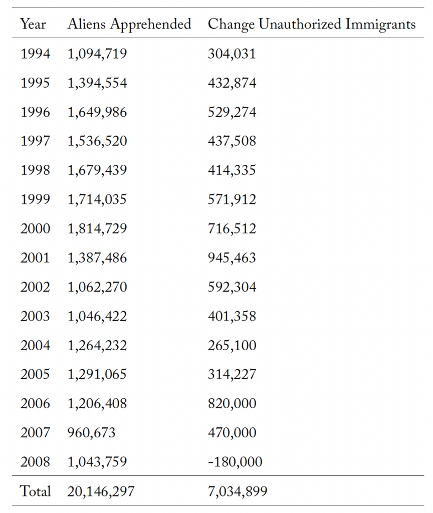
C.1 Econometric evidence and estimation of a lower bounds on $\rho$

The model is estimated for the period 1994-2008. The results of using
two-stage least squares are

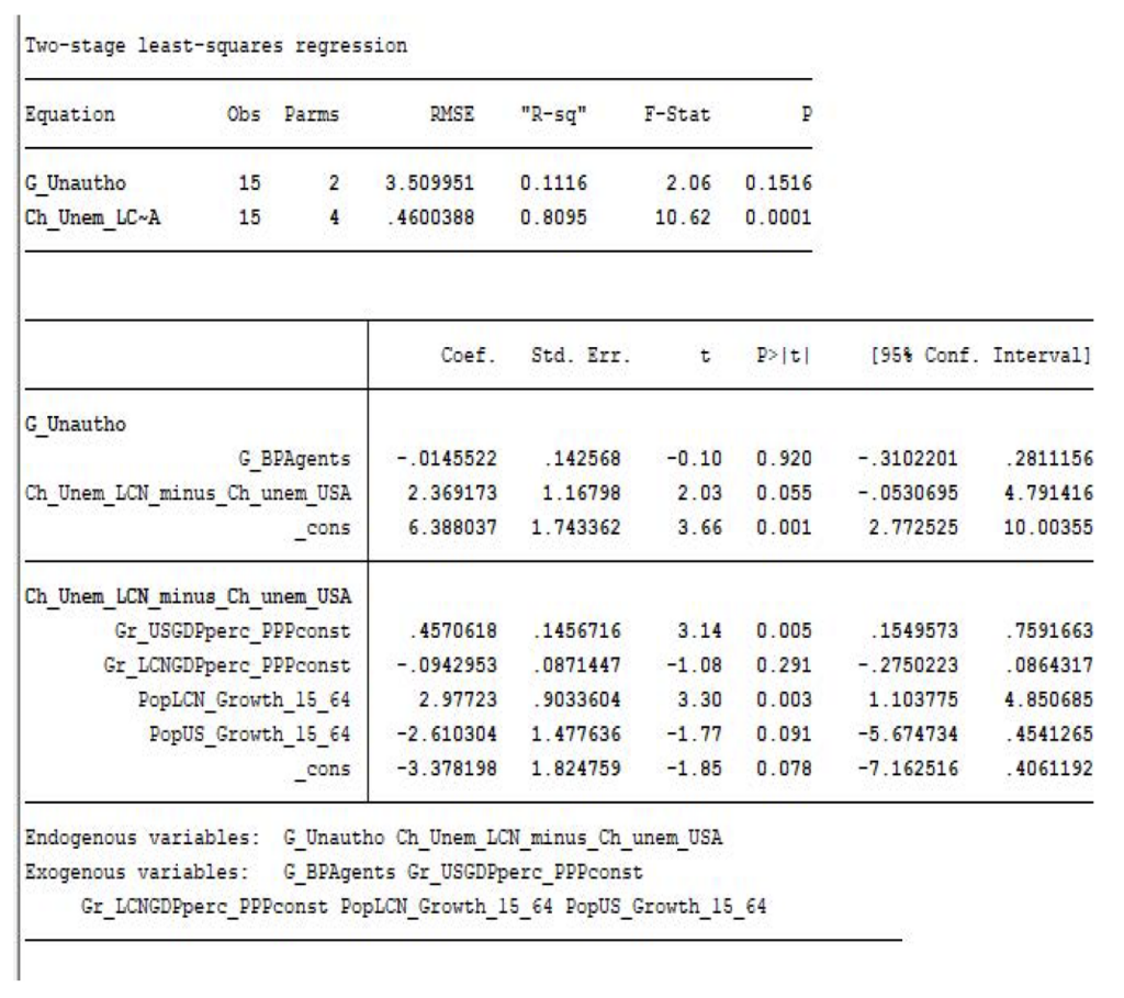
The coefficient we are interested in ( $\gamma_{1}$ ) is significant, estimated at a level of 2.369. The proxy variable capturing the growth in the immigration pool was well explained with an $R^{2}$ of $81\%$ , and although not all the variables are significant at the $95\%$ level of significance, they all have the correct sign: growth in US GDP per capita increases the (proxy of the) pool of unauthorized immigrants, higher GDP per capita in Latin America is associated with a lower immigration pool, population growth in the US is negatively associated with the immigration pool, and higher population growth in the Latin American countries is associated positively with the immigration pool.

If the system is estimated by means of using three-stage least squares, all of the explaining variables of the proxy for the growth in the immigration pool are significant and with the correct sign, with very small variation in the estimated coefficients.

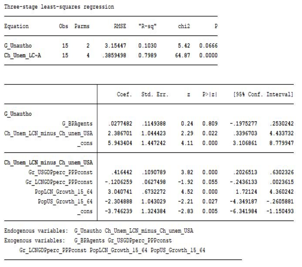
Given these magnitudes, the estimate for the lower bound on $\rho$ is given by

$\widehat{\rho}{lb}=\left( \frac{1-\widetilde{\mu}}{\widetilde{\mu}}\right) \left( \frac{1}{\widehat{\gamma}{1}-1}\right) =\left( \frac{1-.2588}{.2588}\right) \left( \frac{1}{2.369-1}\right) =2.09.$

C.2 Data description

Unauthorized Immigrants. The data was constructed from two sources. First, it was acquired from the website of the Department of Homeland Security (DHS) at https://www.dhs.gov/immigration-statistics/population-estimates/unauthorized-resident, where the relevant series is available since year 2005. For previous years, the data comes from Warren and Warren (2013), who have available data since 1990. The data from DHS is very similar but not identical to the overlapping years produced by DHS, so the final series used for the levels is constructed from the growth factors from the DHS series since 2006, and then applied to the series produced by Warren and Warren for years 2006, 2007, and 2008.

Alien Apprehensions. The time series on aliens apprehended is obtained from the 2019 Yearbook of Immigration Statistics, Table 33, from the website of the Department of Homeland Security, available at https://www.dhs.gov/immigration-statistics/yearbook/2019.

Unemployment, Population and Income per capita Series. The data for unemployment for Latin American and Caribbean countries (LCN) comes from the World Bank’s World Development Indicators. The series for unemployment is SL.UEM.TOTL.ZS and was obtained for LCN and for the US. For the construction of the growth rates in population, the time series used reflects the population aged 15-64 for LCN countries and for the US, series SP.POP.GROW. Finally, for the construction of growth of income per capita, the levels are obtained both for LCN countries and the US, using the series NY.GDP.PCAP.PP.KD, which reports income per capita in constant purchasing parity dollars of 2017.

Border Patrol Agents. Data on the number of agents working on the Border Patrol is available at the website of the US Custom and Border Protection, at https://www.cbp.gov/sites/default/files/assets/documents/2019-Mar/Staffing\%20FY1992-FY2018.pdf.

D Calibration under Constrained Skilled-Based Immigration

Consider the system of first-order conditions when there exists an extra constraint such that $\theta_{s}\leq\theta_{s}^{\max}.$ Assuming that this constraint is binding (and thus the optimal level $\theta_{s}^{\ast}$ in (29) is not feasible), then the constrained solution ( $b^{c},$ $\theta_{s}^{c},$ $\theta_{F}^{c},$ $\theta_{u}^{c},$ $g^{c},\mu {1}^{c},\mu{2}^{c})$ with Lagrangian multipliers $\mu_{1}^{c},$ $\mu_{2} ^{c}$ , as in Appendix A.1, is characterized by the system

(60) $\begin{align*} b &: u^{\prime}\left( b^{c}\right) = \mu_{1}\left( 1+\theta_{F}^{c} +\theta_{s}^{c} +\theta_{u}^{c}\right) \nonumber \\ g &: \alpha v^{\prime}\left( g^{c}\right) = \mu_{2}\left( 1+\theta_{F}^{c} +\theta_{s}^{c} +\theta_{u}^{c}\right) \nonumber \\ \theta_{s} &: \mu_{1}^{c}\left[ \tau w_{s}-b^{c}\right] -\mu_{2}^{c} g^{c} > 0 \text{ when } \theta_{s}^{c}=\theta_{s}^{\max} \text{ (if } \theta_{s}^{\ast}>\theta_{s}^{\max}\text{)} \nonumber \\ \theta_{F} &: \gamma\widetilde{v}^{\prime}\left( \theta_{F}\right) +\mu_{1}^{c}\left[ \tau w_{F}-b\right] = \mu_{2}^{c}g^{c} \nonumber \\ \theta_{u} &: \mu_{1}^{c}\left[ \tau w_{u}-b^{c}+\xi wh^{\prime}\right] = \mu_{2}^{c}g^{c} \nonumber \\ \mu_{1} &: \tau\left( w_{F}\theta_{F}^{c} + w_{s}\theta_{s}^{c} + w + w_{u}\theta_{u}^{c}\right) = b^{c}\left( 1+\theta_{F}^{c} +\theta_{s}^{c} +\theta_{u}^{c}\right) + \xi w\theta_{u}^{\max}h \nonumber \\ \mu_{2} &: G = g^{c}\left( 1+\theta_{F}^{c} +\theta_{s}^{c} +\theta_{u}^{c}\right) \nonumber \end{align*}$

Using (i) log-utility, (ii) an $h\left( \cdot\right)$ function $h=\left( 1-\frac{\theta_{u}}{\theta_{u}^{\max}}\right) ^{\rho}$ and (iii) identifying $\xi$ with $A^{-\rho}$ yields

(61) $\begin{align*} \frac{1}{b^{c}} &= \mu_{1}\left( 1+\theta_{F}^{c}+\theta_{s}^{c}+\theta_{u}^{c}\right) \nonumber \\ \frac{\alpha}{g} &= \mu_{2}\left( 1+\theta_{F}^{c}+\theta_{s}^{c}+\theta_{u}^{c}\right) \nonumber \\ \theta_{s}^{c} &= \theta_{s}^{\max} \nonumber \\ \mu_{2}^{c}g^{c} &= \frac{\gamma}{\theta_{F}^{c}}+\mu_{1}^{c}\left[ \tau w_{F}-b^{c}\right] \nonumber \\ \mu_{2}^{c}g^{c} &= \mu_{1}^{c}\left[ \tau w_{u}-b^{c}+A^{-\rho} w\rho\left( 1-\theta_{u}^{c}/\theta_{u}^{\max}\right)^{\rho-1}\right] \nonumber \\ \tau\left( w_{F}\theta_{F}^{c}+w_{s}\theta_{s}^{c}+w+w_{u}\theta_{u}^{c}\right) &= b^{c}\left( 1+\theta_{F}^{c}+\theta_{s}^{c}+\theta_{u}^{c}\right) +\frac{w\theta_{u}^{\max}}{A^{\rho}}\left( 1-\theta_{u}^{c}/\theta_{u}^{\max}\right)^{\rho} \nonumber \\ G &= g^{c}\left( 1+\theta_{F}^{c}+\theta_{s}^{c}+\theta_{u}^{c}\right) \nonumber \end{align*}$

From the first and second equations above, the Lagrangian multipliers $\mu_{1}^{c}$ and $\mu_{2}^{c}$ are

$\mu_{1}^{c} = \frac{1}{b^{c}\left( 1+\theta_{F}^{c}+\theta_{s}^{c}+\theta_{u}^{c}\right)},$

$\mu_{2}^{c} = \frac{\alpha}{g^{c}\left( 1+\theta_{F}^{c}+\theta_{s}^{c}+\theta_{u}^{c}\right)}.$

Replacing the multipliers $\mu_{1}^{c},$ $\mu_{2}^{c}$ in the fourth equation above yields the expression

$\frac{\gamma}{\theta_{F}^{c}} + \frac{\left[ \tau w_{F} - b^{c}\right]}{b^{c}\left( 1+\theta_{F}^{c} + \theta_{s}^{c} + \theta_{u}^{c}\right)} = \frac{\alpha g^{c}}{g^{c}\left( 1+\theta_{F}^{c} + \theta_{s}^{c} + \theta_{u}^{c}\right)}$

Now solve for $\theta_{F}^{c}$ in order to obtain

(62) $\begin{equation*}\theta_{F}^{c}=\frac{\gamma b^{c}\left( 1+\theta_{u}^{c}+\theta_{s}^{\max}\right) }{\left[ b^{c}\left( 1+\alpha-\gamma\right) -\tau w_{F}\right]}. \end{equation*}$

Using the multipliers $\mu_{1}^{c},$ $\mu_{2}^{c}$ in the fifth equation yields the following equation for $b^{c}$

(63) $\begin{equation*}b^{c}=\frac{\tau w_{u}+A^{-\rho}w\rho\left( 1-\theta_{u}^{c}/\theta_{u}^{\max}\right) ^{\rho-1}}{\left( 1+\alpha\right) }\end{equation*}$

Replace $b^{c}$ from (63) into (62), using $\theta_{s}^{c}=\theta_{s}^{\max}$ which yields

(64) $\begin{equation*}\theta_{F}^{c}=\frac{\gamma\left( 1+\theta_{u}^{c}+\theta_{s}^{\max}\right)\left[ \tau w_{u}+\left( \frac{w\rho}{A^{\rho}}\right) \left(1-\frac{\theta_{u}^{c}}{\theta_{u}^{\max}}\right) ^{\rho-1}\right] }{\left(1+\alpha-\gamma\right) \left[ \tau w_{u}+\left( \frac{w\rho}{A^{\rho}}\right) \left( 1-\frac{\theta_{u}^{c}}{\theta_{u}^{\max}}\right) ^{\rho-1}\right] -\left( 1+\alpha\right) \tau w_{F}}.\end{equation*}$

Inserting $b^{c}$ from (63) into the sixth equation and setting $\theta_{s}^{c}=\theta_{s}^{\max}$ yields

(65) $\begin{align*}\left( 1+\alpha\right) \tau\left( w_{F}\theta_{F}^{c}+w_{s}\theta_{s}^{\max}+w+w_{u}\theta_{u}^{c}\right) & =\left[ \tau w_{u}+\left(\frac{w\rho}{A^{\rho}}\right) \left( 1-\frac{\theta_{u}^{c}}{\theta{u}^{\max}}\right) ^{\rho-1}\right] \left( 1+\theta{F}^{c}+\theta{s}^{\max}+\theta{u}^{c}\right) \& +\left( 1+\alpha\right) \left( \frac{w}{A^{\rho}}\right) \theta{u}^{\max}\left( 1-\frac{\theta{u}^{c}}{\theta_{u}^{\max}}\right) ^{\rho}\nonumber\end{align*}$

Thus, if the interest was in computing $\theta_{F}^{c}$ and $\theta_{u}^{c},$ equations (64) and (65) form a system of two equations in these two unknowns.

For the calibration of ${A,\alpha,\gamma}$ , it is necessary to have one more equation, which is provided by the unconstrained solution to $\theta_{s} ^{\ast}$ obtained previously and which is assumed not to be observable. Start from legal immigration in (28) and then replace (27) to obtain the expression

$\theta_{s}^{\ast} = \frac{w_{s}\left( 1+\theta_{u}^{\ast}\right) \left( 1+\gamma\right) - \left( 1+\alpha\right) \left[ \left( w-\frac{E^{\ast}}{\tau}\right) + w_{u}\theta_{u}^{\ast}\right]}{w_{s}\left( \alpha - \gamma\right)} - \frac{\gamma\left[ \left( \frac{E^{\ast}}{\tau} + w_{s} - w\right) + \left( w_{s} - w_{u}\right) \theta_{u}^{\ast}\right]}{\left( w_{s} - w_{F}\right) \left( \alpha - \gamma\right)}$

The above expression can be rewritten as

$\theta_{s}^{\ast} = a_{1}\left( 1+\theta_{u}^{\ast}\right) + a_{2}\left( w-w_{u}-\frac{E^{\ast}}{\tau}\right)$

for constants $a_{1}$ and $a_{2}$ that depend on parameters $\left{ \alpha,\gamma,w_{u},w_{s},w_{F}\right}$ , given by

(66) $\begin{align*} a_{1} &= \left( \frac{1}{\alpha-\gamma}\right) \left[ \left( 1+\gamma\right) -\left( 1+\alpha\right) \left( \frac{w_{u}}{w_{s}}\right) -\gamma\left( \frac{w_{s}-w_{u}}{w_{s}-w_{F}}\right) \right], \nonumber \\ a_{2} &= \left( \frac{1}{\alpha-\gamma}\right) \left[ \frac{\gamma}{\left( w_{s}-w_{F}\right)} -\frac{\left( 1+\alpha\right)}{w_{s}} \right]. \nonumber \end{align*}$

Finally replace the unconstrained level $\theta_{u}^{\ast}$ given by (18), and since optimal enforcement in the unconstrained case is $E^{\ast}=A^{\rho}w\theta_{u}^{\max}\left( 1-\frac{\theta_{u}} {\theta_{u}^{\max}}\right) ^{\rho}$ , we obtain

(67) $\begin{equation*}\theta_{s}^{\ast}=\left{ 1+\theta_{u}^{^{{\max}}}\left[ 1-\left( \frac{\tau A^{\rho}\left( w{s}-w_{u}\right) }{w\rho}\right) ^{\frac{1}{\rho-1}}\right] \right} a_{1}+a_{2}\left( w-w_{u}-\frac{\frac{w}{A^{\rho}}\theta_{u}^{\max}\left( \frac{\tau A^{\rho}\left( w_{s}-w_{u}\right) }{w\rho}\right) ^{\frac{\rho}{\rho-1}}}{\tau}\right)\end{equation*}$

Thus, when immigration quotas are the targets, then (64), (65), and (67) form a non-linear system of three equations in the unknowns $\left{ A,\alpha,\gamma\right}$ . The system takes targets $\left{ \theta_{F}^{c},\theta_{u}^{c},\theta_{s}^{\ast}\right}$ and parameters $\left{ w,w_{F},w_{s},w_{u},\tau,\rho,\theta_{u}^{\max} ,\theta_{s}^{\max}\right}$ and produces calibrated values of $\left{ \widehat{A}{c},\widehat{\alpha}{c},\widehat{\gamma}_{c}\right} .$

Setting $\theta_{F}^{c}=.0321,$ $\theta_{u}^{c}=.0307$ and $\theta_{s}^{\ast }=.025$ and setting $w=1,$ $w_{F}=0.8,$ $w_{s}=1.25,$ $w_{u}=0.75,$ $\tau=0.3,$ $\rho=3,$ $\theta_{u}^{\max}=.25,$ $\theta_{s}^{\max}=.0081$ , the non-linear solver yields $\widehat{A}{c}=2.4966$ , $\widehat{\alpha} {c}=0.303164$ and $\widehat{\gamma}_{c}=0.013952.$

Finally, in order to verify the quality of the solution, a target of $\theta_{s}^{\ast}=.0081$ can be selected so that $\theta_{s}^{\ast} =\theta_{c}^{\ast}=.0081$ , then the non-linear solver yields the same calibrated values as in the unconstrained calibration, so that in that case $\widehat{A}{c}=\widehat{A}=2.4874,$ $\widehat{\alpha}{c}=\widehat{\alpha }=.30945$ and $\widehat{\gamma}_{c}=\widehat{\gamma}=.01413$ .

References

[1] Acemoglu, Daron, and David Autor (2012). ”What Does Human Capital Do? A Review of Goldin and Katz’s The Race between Education and Technology,” Journal of Economic Literature 50(2), 426–63.

[2] Ales, Laurence (2020). ”Comments on ’What is the Optimal Immigration Policy? Migration, Jobs and Welfare’ by Guerreiro, Rebelo and Teles,” Journal of Monetary Economics 113, 88–91.

[3] Alesina, Alberto, Armando Miano, and Stefanie Stantcheva (2023). ”Immigration and Redistribution,” The Review of Economic Studies 90(1): 1–39. https://doi.org/10.1093/restud/rdac011

[4] American Immigration Council (2021). ”How the United States Immigration System Works.” Available at https://www.americanimmigrationcouncil.org/research/how-unitedstates-immigration-system-works.

[5] Aydemir, Abdurrahman (2011). ”Immigrant Selection and Short-term Labor Market Outcomes by Visa Category,” Journal of Population Economics 24, 451–475.

[6] Bandyopadhyaya, Subhayu, and Santiago M. Pinto (2017). ”Unauthorized Immigration and Fiscal Competition,” European Economic Review 92, 283–305.

[7] Barcellos, Silvia H. (2010). ”Legalization and the Economic Status of Immigrants,” WR-754, Rand Labor and Population Working Paper.

[8] Benhabib, Jess (1996). ”On the Political Economy of Immigration,” European Economic Review 40, 1737–1743.

[9] Benhabib, Jess, and Boyan Jovanovic (2012). ”Optimal Migration: A World Perspective,” International Economic Review 53, 321–348.

[10] Ben-Gad, Michael (2018). ”On the Political Economy of Deficit Bias and Immigration,” The Economic Journal, 128(614), 2191–2221. doi: 10.1111/ecoj.12502

[11] Blau, Francine D., and Christopher Mackie. (2017). National Academies of Sciences, Engineering, and Medicine. ”The Economic and Fiscal Consequences of Immigration.” Washington, DC: The National Academies Press. https://doi.org/10.17226/23550.

[12] Bohn, Henning, and Armando R. Lopez-Velasco (2019). ”Immigration and Demographics: Can High Immigrant Fertility Explain Voter Support for Immigration,” Macroeconomic Dynamics 23(5), 1815–1837.

[13] Bohn, Henning, and Armando R. Lopez-Velasco (2018). ”Intergenerational Mobility and the Political Economy of Immigration,” Journal of Economic Dynamics and Control 94, 72–88.

[14] Bond, Eric, and Tain-Jy Chen (1987). ”The Welfare Effects of Illegal Immigration,” Journal of International Economics, 23, 315–328.

[15] Borjas, George (2001). ”Heaven’s Door: Immigration Policy and the American Economy.” Princeton, NJ: Princeton University Press.

[16] Borjas, George J., and Rachel M. Friedberg (2009). ”Recent Trends in the Earnings of New Immigrants to the United States,” NBER Working Paper W15406.

[17] Card, David, Christian Dustmann, and Ian Preston (2012). ”Immigration, Wages, and Compositional Amenities,” Journal of the European Economic Association 10, 78–119.

[18] Chassambouli, Andri, and Giovanni Peri (2015). ”The Labor Market Effects of Reducing the Number of Illegal Immigrants,” Review of Economic Dynamics 18, 792–821.

[19] Chassambouli, Andri, and Giovanni Peri (2020). ”The Economic Effects of Immigration Policies: Analyzing and Simulating the US Case,” Journal of Economic Dynamics and Control 114, 103898.

[20] Cohn, D’Vera (2015). ”How U.S. Immigration Laws and Rules Have Changed Through History.” Pew Research Center. Available at https://www.pewresearch.org/shortreads/2015/09/30/how-u-s-immigration-laws-and-rules-have-changed-through-history/.

[21] Dolmas, Jim, and Gregory Huffman (2004). ”On the Political Economy of Immigration and Income Redistribution,” International Economic Review 45, 1129–1168.

[22] Ethier, Wilfred J. (1986). ”Illegal Immigration: The Host Country Problem,” The American Economy Review 76, 56–71.

[23] Facchini, Giovanni, and Cecilia Testa (2021). ”The Rhetoric of Closed Borders: Quotas, Lax Enforcement, and Illegal Immigration,” Journal of International Economics 129, 103415.

[24] Guerreiro, Joao, Sergio Rebelo, and Pedro Teles (2020). ”What is the Optimal Immigration Policy? Migration, Jobs, and Welfare,” Journal of Monetary Economics 113, 61–87.

[25] Guzman, Mark, Joseph Haslag, and Pia Orrenius (2008). ”On the Determinants of Optimal Border Enforcement,” Economic Theory 34, 261–296.

[26] Haupt, Alexander, and Wolfgang Peters (1998). ”Public Pensions and Voting on Immigration,” Public Choice 95, 403–413.

[27] Kandel, William A., Jill H. Wilson, and Sarah A. Donovan (2022). ”US Employment- Based Immigration Policy.” US Congressional Research Service Report R47164. Available at https://crsreports.congress.gov/product/pdf/R/R47164.

[28] Kerr, Sari Pekkala and William R. Kerr (2011). ”Economic Impacts of Immigration: A Survey,” NBER Working Paper 16736.

[29] Kolker, Abigail F. (2022). ”Unauthorized Immigrants’ Eligibility for Federal and State Benefits: Overview and Resources.” US Congressional Research Service Report R47318. Available at https://crsreports.congress.gov/product/pdf/R/R47318.

[30] Kossoudji, Sherrie A. and Deborah Cobb-Clark (2002). ”Coming Out of the Shadows: Learning about Legal Status and Wages from the Legalized Population,” Journal of Labor Economics 20(3), 598–628.

[31] Lindbeck, Assar and J¨orgen W. Weibull (1987). ”Balanced-budget Redistribution as the Outcome of Political Competition,” Public Choice 52(3), 273–297.

[32] Lopez-Velasco, Armando R. (2023) ”A Snapshot of Immigration Flows into the US.” Center for Border Economic Studies (CBest) Border Business Briefs, Fall 2023. Available at https://www.utrgv.edu/cbest/publications/index.htm.

[33] Mayda, Anna Maria (2006). ”Who is Against Immigration? A Cross-Country Investigation of Individual Attitudes Toward Immigrants,” The Review of Economic Statistics 88, 510–530.

[34] Massey, Douglas S. and Karen A. Pren (2012). ”Unintended Consequences of US Immigration Policy: Explaining the Post-1965 Surge from Latin America,” Population and Development Review 38, 1–29. https://doi.org/10.1111/j.1728-4457.2012.00470.x

[35] Migration Policy Institute (2013). ”Major US Immigration Laws, 1790-Present.” Washington, DC: Migration Policy Institute. Available at https://www.migrationpolicy.org/research/majorus-immigration-laws-1790-present.

[36] OECD (2017). ”Making Integration Work: Family Migrants.” Paris: OECD Publishing. http://dx.doi.org/10.1787/9789264279520-en.

[37] Ortega, Francesc (2005). ”Immigration Quotas and Skill Upgrading,” Journal of Public Economics 89, 1841–1863.

[38] Passel, Jeffrey S. and Barry Edmonston (1994). ”Immigration and Race: Recent Trends in Immigration to the United States.” In B. Edmonston and J.S. Passel (Editors), Immigration and Ethnicity: Immigration and the Adjustment of America’s Newest Immigrants. Washington, D.C.: The Urban Institute.

[39] Persson, Torsten and Guido Tabellini (2002). ”Political Economics: Explaining Economic Policy.” Cambridge, MA: MIT Press.

[40] Razin, Assaf, Efraim Sadka, and Benjarong Suwankiri (2011). ”Migration and theWelfare State: Political-economy Policy Formation.” Cambridge, MA: MIT Press.

[41] Rivera-Batiz, Francisco L. (1999). ”Undocumented Workers in the Labor Market: an Analysis of the Earnings of Legal and Illegal Mexican Immigrants in the United States,” Journal of Population Economics 12, 91–116.

[42] Sand, Edith and Assaf Razin (2007). ”The Role of Immigration in Sustaining the Social Security System: a Political Economy Approach.” CESifo Working Paper 1979.

[43] Smith, James P. and Barry Edmonston. (1997). ”The New Americans: Economic, Demographic, and Fiscal Effects of Immigration.” Washington, DC: The National Academies Press. https://doi.org/10.17226/5779.

[44] Straut-Eppsteiner, Holly (2022). ”Citizenship and Immigration Statuses of the U.S. Foreign- Born Population.” US Congressional Research Service, Focus Report IF11806. Available at https://crsreports.congress.gov/product/pdf/IF/IF11806.

[45] Storesletten, K. (2000). ”Sustaining Fiscal Policy through Immigration,” Journal of Political Economy, 108(2), 300–323. https://doi.org/10.1086/262120

[46] Warren, R. and J. R. Warren (2013). ”Unauthorized Immigration to the United States: Annual Estimates and Components of Change, by State, 1990 to 2010,” International Migration Review 47(2), 296–329.

[47] Wasem, Ruth Ellen (2014). ”Unauthorized Aliens Residing in the United States: Estimates Since 1986.” US Congressional Research Service, Focus Report RL33874. Available at https://crsreports.congress.gov/product/pdf/RL/RL33874.

Executive Summary

Resources

Related Publications

Related News

Related Blogs

Focuses