Keeping a Clean Reputation: More Evidence on the Perverse Effects of Disclosure

Tracy, Dustin; Deck, Cary

1 Introduction

Lawyers, financial advisors, doctors, and other agents are said to have conflicts of interest if their personal motivation is at odds with their professional responsibilities to serve their clients (Boatright, 2000a,b). While there are various policies in place requiring disclosure of conflicts of interest, survey literature reveals such conflicts are common and undermine trust in professionals. For example, Scholl and Hung (2018) find there is generally low trust in financial professionals. They report that while 51% of consumers would prefer their adviser not have a conflict of interest, many consumers lacked awareness of financial advisers’ responsibilities or their compensation structure. Ninety-four percent of doctors have a financial relationship with a pharmaceutical company, according to Campbell et al. (2007). They report that most (83%) doctors received gifts including meals from pharmaceutical companies, and many received funding for continuing education or conference attendance (35%) or payment for speaking or research activity (28%). Interestingly, Mainous (1995) finds that patients viewed personal gifts to physicians less favorably than office-use gifts, believing the former could impact the cost of care. Further, patients who believe physicians accept gifts from the pharmaceutical industry trust doctors significantly less than those patients who do not believe physicians accept gifts (Grande et al., 2012). Unsurprisingly, physicians believe that gifts from the pharmaceutical industry are less influential and more acceptable compared to patient attitudes (Gibbons et al., 1998).

The propensity for experts to behave in a manner that conflicts with the interest of the principal they represent has been established in economics through both lab and field experiments (see Kerschbamer and Sutter (2017) for a review of this literature). The conventional wisdom is that if a principal is aware of an agent’s conflict of interest then the principal can take appropriate counteraction. As stated by Cain et al. (2005, p. 2), “Common sense suggests that recipients of advice will benefit from being more fully informed when they are made aware of an advisor’s conflict of interest.” This notion has led to widespread requirements for principals to disclose conflicts of interest, particularly in markets for “credence goods,” where the agent is not able to determine the quality of service provided even after the fact.¹ While there is general support for the disclosure of conflicts of interest, there is some debate about the potential impact. For example, a majority of patients report wanting to know if their doctor received a gift over $100 from a pharmaceutical company, a majority also say their trust in their doctor would be undermined if they knew their doctor had received such a gift (Green et al., 2012). Rose et al. (2019) find that disclosing physicians’ financial relations within the healthcare industry improved patient awareness of those relationships, but actually had no impact on the likelihood of attending an appointment or stated trust and confidence in physicians. In Massachusetts, a disclosure law reduced prescriptions for both branded and generic antidepressants, antipsychotics, and statins (Guo and Sriram, 2017). However, the 2012 Federal sunshine law had little impact on average payments from pharmaceutical companies to prescribers and instead led to higher payments to fewer doctors (Guo et al., 2017). Similarly, Chen et al. (2019) find that in states with laws requiring posted public disclosure, payments to physicians who accepted less than $100 decreased. However, payments to physicians who accepted more than $100 increased.

In a creative experiment, Cain et al. (2005) show that disclosure can exacerbate the problem introduced by a conflict of interest rather than reducing it. In their study, agents provided estimates of the value of a jar of coins to principals. Principals were paid based on the accuracy of their own guess as to the value of the coins in the jar, but agents who had a conflict of interest were paid based on how large the principal’s estimate was. Cain et al. (2005) find that in the absence of disclosure, agents provide upwardly biased estimates. This bias leads principals to substantially overestimate the value of the coins. When the conflict of interest was disclosed to principals, the upward bias exhibited by agents did not decrease, but rather was dramatically increased. While the principals correctly anticipated agents would provide upwardly biased estimates, the principals badly underestimated the magnitude of the bias and thus the net effect of disclosure was actually harmful to the principals.

While the counter-intuitive finding of Cain et al. (2005) suggests that it may be optimal to not disclose conflicts of interest, their setting is one in which there are no other pressures on the agents. Becker (1968) argues that when dishonest behavior has little to no cost it is expected to be prevalent; so, the observed bias in Cain et al. (2005) in the absence of disclosure is unsurprising. But in everyday life many circumstances involve reputation concerns, and the fear of lost future opportunities makes dishonesty costly for agents. The expected effect of maintaining a reputation is straightforward in cases where the principal can easily assess the performance of an agent ex post, but for credence goods, such as selecting a doctor, financial adviser, or lawyer, the effect is less obvious since assessing the agent is difficult. Still, Darby and Karni (1973) discuss how market forces and reputation can limit fraud for credence goods, and Wolinsky (1993) presents a theoretical proof of how reputation and consumer search can discipline experts.

However, the empirical support for the effectiveness of reputations is less clear. For example, Pope (2009) finds patients select hospitals based on rankings, but not underlying quality measures of care. Hannan et al. (1994) argue providing rankings improves quality and decreases mortality rates for coronary artery bypass graft surgery. But, Mukamel and Mushlin (1998) find the rankings increased market share for low mortality surgeons and hospitals, leading to increased prices for the more highly demanded providers. Dranove et al. (2003) claim that rankings reduce consumer welfare, at least in the short term, as doctors attempting to improve their reputations elect to operate on healthier patients; this pattern leads to increased costs, and results in no improvement in the outcomes of the healthier patients, but worse outcomes for less healthy patients. Outside of healthcare, Carl (2008) finds that disclosure of payments increases an agent’s credibility when engaged in word-of-mouth product promotion, a potential channel through which disclosure could be harmful. It is also possible that disclosure actually creates confusion, thus generating another path by which disclosure could be harmful. For home mortgages, Ben-shahar and Schneider (2011) argue that people may not know how to use disclosed information and that they can only pay attention to so many things, so that it is better for the principals if they are focused on a limited number of key features of the decision.

If reputation is sufficient to discipline agents, it is unclear if disclosure is socially desirable; the upside benefit is limited and disclosure could actually introduce self-serving bias in assessments. Of course, if agents exhibited biased assessments even in the presence of reputation concerns, then it is still possible that disclosure could be either beneficial, as typically assumed, or harmful, as suggested by some. In this paper we use a controlled laboratory experiment inspired by Cain et al. (2005) to examine the impact of disclosure on self-serving bias in assessments by agents in a credence-good setting where agents have reputation concerns. In our task, principals are forced to select between two options of unknown value (jars with indeterminate compositions of coins), but have to rely on an agent’s assessment of the value of those options. The principal receives a benefit based on the value of the selected option and a noisy signal of the value of the non-selected option, both of which are independent of their agent’s behavior. Principals can rate agents after their interaction and can use the ratings provided by other principals when selecting an agent. Agents have a financial incentive to encourage a principal to select a particular option (jar of coins), but the agents also have an incentive for principals to choose to solicit their assessments. There are two treatments in the experiment: one in which the agents’ conflict of interest is not disclosed to the principal and one in which it is disclosed. We measure bias as a systematic overstatement by the agent of the value of the conflicted option in comparison to the other option. Thus, our use of the term bias coincides with both the statistical definition and the colloquial one. We find that, when there is no disclosure we do not observe systematically biased assessments of values. But, like Cain et al. (2005), when disclosure is introduced we find that agents do provide systematically biased assessments of value and principals are unable to fully incorporate this fact into their decision making.

2 Experimental Design and Hypotheses

In this section we lay out the experimental design including the task and procedures. We also present a simple theoretical model that serves as the basis for our hypothesis.

2. 1 Main Experimental Task and Treatments

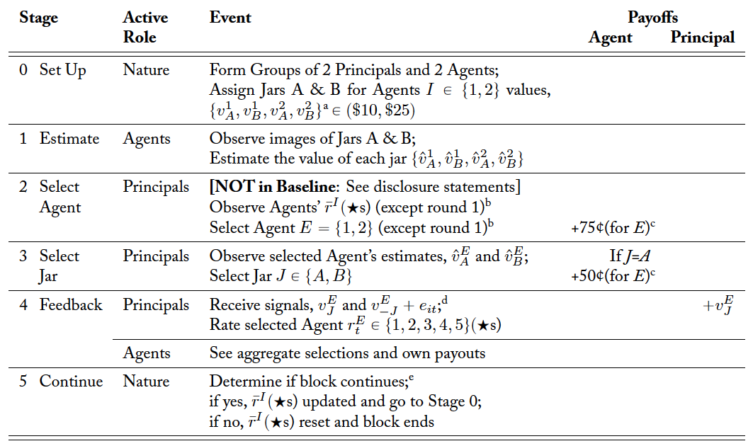
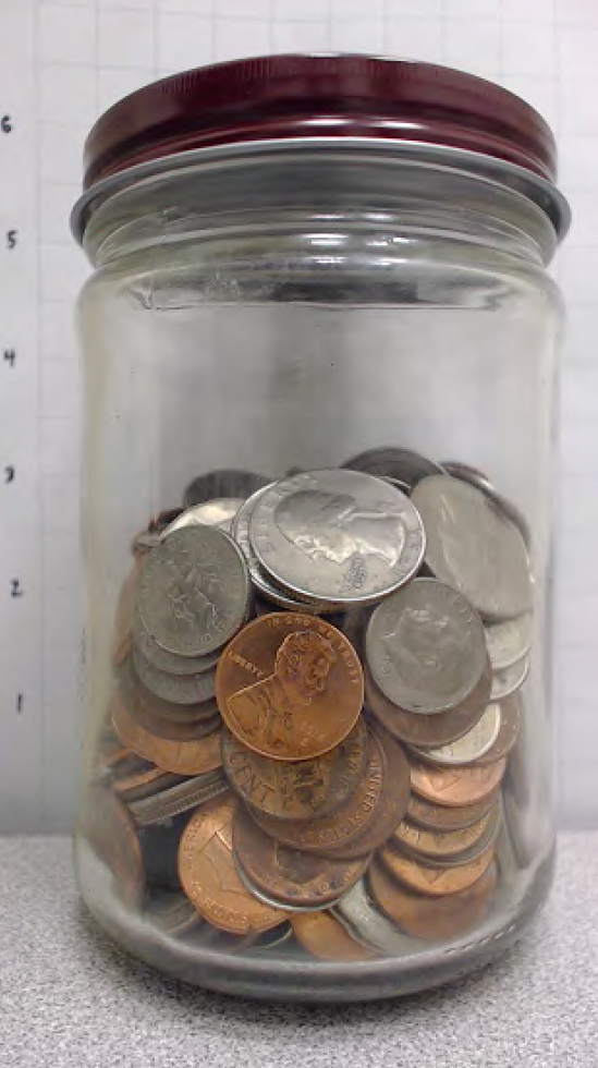
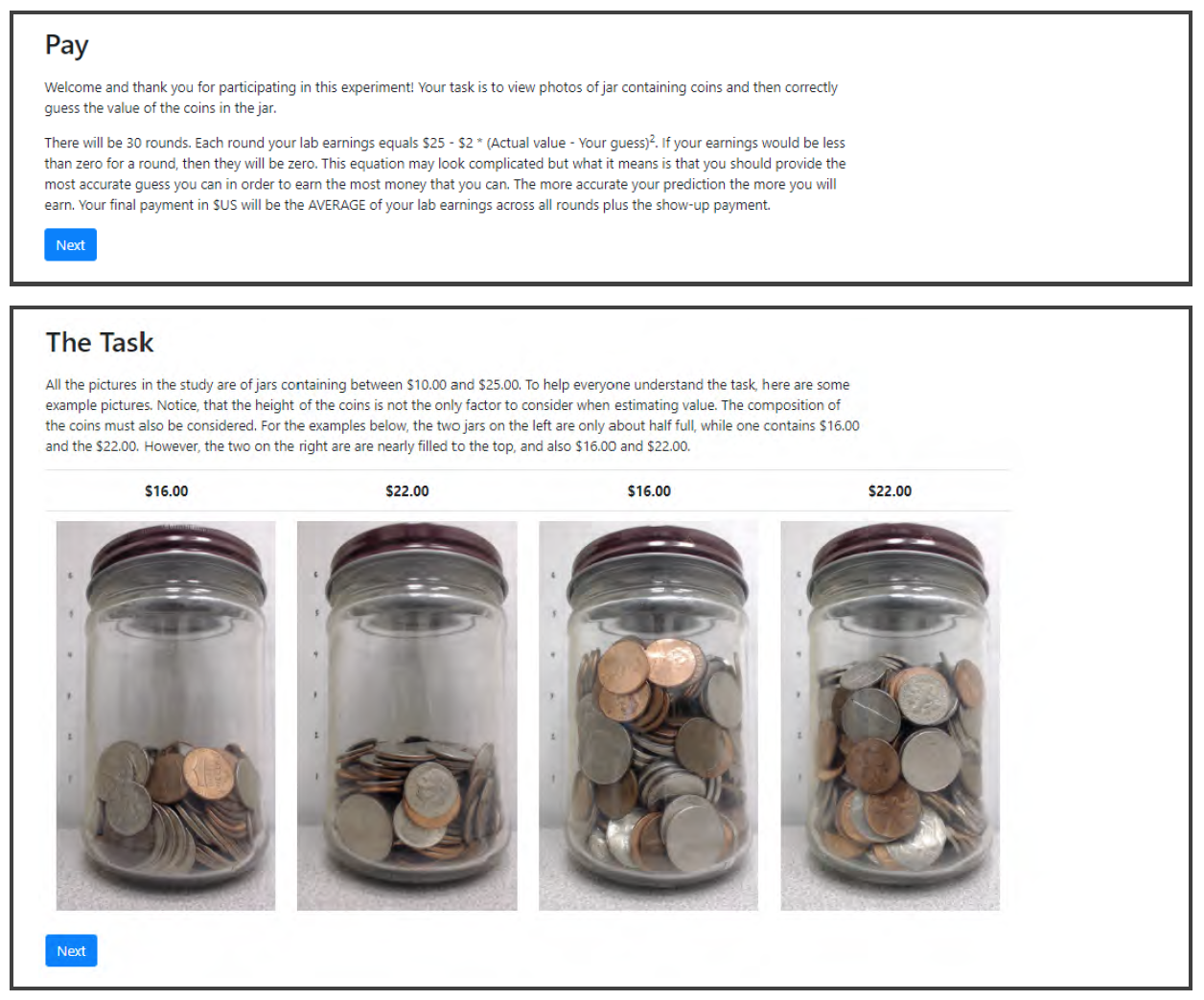
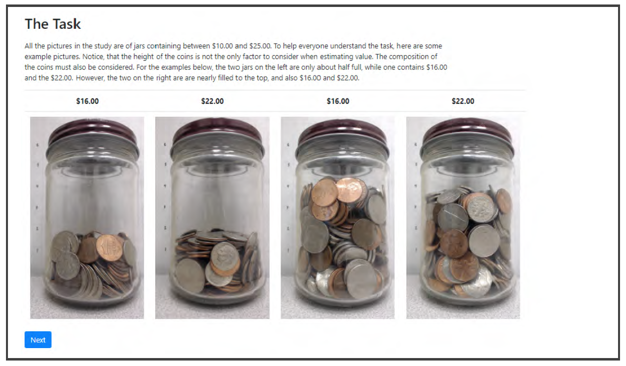
Our experiment varies whether or not the agents’ conflict of interest is disclosed in an environment in which an agent’s future earning can be diminished by an unfavorable reputation. In the main experimental task, a principal (“investor” in the subject interface) must select between two options labeled A and B. The options are jars of coins and the principal’s value for an option equals the value of the coins in the associated jar. However, the principal cannot observe the jars directly and instead is forced to rely upon an assessment of the value of each option provided by an agent (“expert” in the subject interface). The agent has a direct incentive to encourage the principal to select option A, but also has an incentive to maintain a good reputation in order to be selected by other principals in the future as the game is played over multiple rounds. The rationale for using jars of coins is that the agent always has plausible deniability, even to the researcher, that the reported estimates of value match the agent’s actual beliefs.²

A session of the experiment involved 12 subjects. Half of the subjects were randomly assigned the role of principal and half were assigned the role of agent. Once assigned, subjects retained their roles throughout the entire experiment, which lasted for multiple blocks of distinct rounds.

Table 1 lists the sequence of events within each round of the experiment. In Stage 0, subjects are randomly assigned to a group consisting of two agents and two principals. Additionally, the value of options A and B were assigned. In Stage 1, the agents observed two images of jars of coins (labeled “Jar A” and “Jar B”).³ Figure 1 provides a sample of one of the images shown to agents in the experiment. After observing the images, each agent would provide an estimate for the value of the coins in each jar. In Stage 2 of each round after the first, principals see the mean number of stars each agent in the group has received over the course of the previous rounds in the current block. In the Disclosure Treatment, agents were also informed that the expert would earn an extra $0.50 if the principal chooses Jar A. In the Baseline, no such disclosure was made although the agents still had the same conflict of interest. The presence or absence of the disclosure statement is the only difference between the two treatments.⁴ The principals then selected an agent, E. An agent earned $0.75 for each principal that selected the agent. In Stage 3, principals observed $\hat{v}^{E}_{A}$ and $\hat{v}^{E}_{B}$ which are the estimated values for Jar A and Jar B provided by the agent selected in Stage 2. Principals then select a jar. The principal’s agent earns an additional $0.50 if the principal selects Jar A. In Stage 4, the value of the selected option, $v^{E}_{J}$ , was revealed to the principal. Each principal also received a noisy signal of the true value of the jar that was not selected. The noisy signal was equal to $v^{E}_{J}+e_{it}$ where $e_{it} \thicksim U[ \textdollar -2.00, \textdollar 2.00]$ . Principals then rated their agent on a scale of 1 to 5 stars, with 1 star being the worst and 5 stars being the best. Each agent was informed of their own payoff, the number of principals who selected the agent, and the number of principals who selected the agent and subsequently selected Jar A. Agents were never informed of the true value of Jars A and B nor were they informed of their own reputation.⁵

Stage 5 determines if a block continues for an additional round or not. For Rounds 1 through 4 of each block, once Stage 4 was completed the process returned to Stage 0 and repeated. However, starting in the 5th round of a block, at Stage 5 the process returned to Stage 0 with a 75% chance and the block ended with a 25% chance. Thus, the horizon of the block was indefinite although subjects knew the stochastic nature of the termination. Importantly, reputations did not carry over between blocks. Thus, a new block offered an agent a chance to start over. This was done out of concern that an agent who formed a bad reputation early might never have the chance to improve it in later rounds since only selected agents are rated. A single set of realizations was drawn and used to determine the duration of each block for all sessions in both treatments. Ultimately, there were four blocks lasting a combined 29 rounds. Agents were paid their cumulative earnings for two randomly chosen blocks whereas principals received the value of the jar selected in one of the 29 rounds chosen at random.

2.2 Additional Experimental Details

The jars that were used contained mixtures of quarters, dimes, nickels and pennies. The actual values of the contents ranged from a low of $13.32 to a high of $22.43 with a mean value of $17.77. Jars contained between 175 and 466 coins each. In the instructions it was demonstrated that volume was not a good indicator of value of coins. The intention was that each image would be used as both Option A and Option B during the course of the experiment although not in the same round to control for jar-specific characteristics. However, due to a programming error, some images were treated as Option A twice or as Option B twice for some subjects. Therefore, the analysis presented in the next section is limited to cases where an image was used both for Option A and Option B over the course of the experiment.⁶

Table 1. Sequence of Events within a Round

^a $v_A^1=v_B^2 \text { and } v_A^2=v_B^1$ .
^b In Round 1, there are no ratings to show, and one agent is assigned to each principal, ensuring ratings in future rounds.
^cThe agent who is not selected earns no payment.
^d $e_{i t} \sim \mathcal{U}(-\$ 2,+\$ 2)$
^e Starting in the 5th round, the block continued for another round with a 75% probability.

The experiment was implemented via oTree (Chen et al., 2016) and conducted at the Economic Science Institute at Chapman University. A copy of the instructions is included in Appendix A.1. Subjects were recruited from the lab’s standing pool of volunteers and none of the subjects had participated in any related study. Each session lasted up to 90 minutes, and subjects earned an average of $22.90 including a $7 participation payment. For both the Baseline and the Disclosure Treatment, three sessions were run involving a total of 72 subjects.

Guessing the correct value of the coins is challenging. As a demonstration, we encourage the reader to guess the value of the coins shown in Figure 1 before reading the footnote for this sentence.⁷ Therefore, a separate study was conducted to calibrate error in estimating the value of each jar of coins. We refer to this separate study as the Guess Experiment. Twenty-four subjects participated in the Guess Experiment in a single session at the Economic Science Institute. This session lasted 30 minutes and relied on volunteers from the same subject pool as the main experiment although no one was allowed to participate in both the Guess Experiment and the main experiment. Subjects in the Guess Experiment observed the full set of images used in the main experiment, and a quadratic scoring rule was used to incentivize truthful reporting of the value of the coins in each image.⁸ The average earnings in the Guess Experiment were $14.58 including the $7 participation payment.

Figure 1. Sample Image

2.3 Theoretical Model

Levitt and List (2007) present a model in which the utility of agent $i$ for an action has additively separate terms for the moral component, $M_i$ , and the financial component, $M_i$ . Specifically, they posit

(1) $\begin{equation*} U_{i}(a,v,n,s)=M_{i}(a,v,n,s)+W_{i}(a,v) \end{equation*}$

where $a$ is the action, $v$ is amount of money at stake, $n$ capture societal norms or laws, and $s$ is the scrutiny the action will receive. For an immoral action the first term will be negative. However, if the second term is greater than the first, the immoral action will bring agent $i$ a net increase in utility and the agent will take the action.

In this model, an increase in scrutiny for a given norm increases the moral cost but it has no impact on the financial benefits (i.e., $\frac{\delta M_{i}}{\delta s} < 0$ and $\frac{\delta W_{i}}{\delta s}=0$ ). Thus, disclosure to the principal that agent $i$ earns a bonus if the principal chooses one option but not the other should increase the moral scrutiny of the estimates $i$ reports, which would discourage immoral action by the agent. With the introduction of a reputation the financial term could also depend on both $n$ and $s$ as well (i.e., $v=f(n,s, \cdots)$ ). In such a setting an immoral action leads to both greater moral costs and reduced financial benefit (i.e., $\frac{\delta M_{i}}{\delta s} < 0$ and $\frac{\delta W_{i}}{\delta v} \frac{\delta v}{\delta s} < 0$ ). This would make disclosure even more attractive for principals.

However Cain et al. (2005) speculate that disclosure may actually create a “moral license” to engage in otherwise socially unacceptable behavior. Effectively, this line of reasoning posits that since the principals have been warned, they should expect agents to engage in self-serving behavior and account for this when making their own decisions. This line of reasoning is similar to the old adage of caveat emptor. In terms of the model by Levitt and List, moral licensing alters the norms, $n$ , such that the immorality of an action is reduced (i.e., $M_{i}(a,v,n_{disclosure},s) > M_{i}(a,v,n_{nondisclosure},s)$ ). If true, the net effect of such moral licensing is ambiguous, and disclosure could lead to more or less self-serving behavior. This ambiguity is true even when taking reputation into account, because the financial harm from an immoral action could be reduced as the norm changes.

Based on this model, our experiment seeks to answer the two following questions which serve as the main hypotheses to be tested. First, will agents exhibit a self-serving bias in the presence of reputation concerns? Second, will the disclosure of the agent’s conflict of interest lead to more self-serving bias on the part of agents?

3 Results

The results are presented in three subsections. The first subsection reports the estimates of jar values from the Guess Experiment, because these serve as a reference point for estimates reported in the main experiment. The second subsection focuses on the behavior of agents in the Baseline and in the Disclosure Treatment, which is the primary focus of the paper and where our two main hypotheses are tested. The third subsection reports exploratory analysis of the behavior of principals in the Baseline and in the Disclosure Treatment.

3.1 Guess Experiment

The mean guess of jar value was $14.61, while the mean of the true values was $17.78. That is, the average error was -$3.17. Figure 2 shows a boxplot of the estimates from the Guess Experiment for each jar, ordered by the actual value of the coins in the jar (not the order in which subjects in either treatment observed the jars). The ˛s show the actual value of a given jar while the thick black line gives the median guess and the gray box shows the interquartile range of guesses. In only 3 out of 30 jars did the median guess not fall below the true value. In fact, for a sizable majority of the jars the true value exceeded the 75th percentile of guesses.⁹ A sign test rejects that errors are unbiased (p-value ă .001). This leads to Finding 1.

Finding 1: People systematically underestimate the value of jars.

Because people so badly underestimate the true value of the jars, it is possible that someone who was deliberately inflating their estimates could still systematically report estimates below the true value. For this reason, we use the estimates from the Guess Experiment as a basis of comparison for identifying agent bias in stated estimates of value in the main experiment. While it is clear from Figure 2 that there is considerable variation across individuals with respect to their estimates of the value of a given jar, if agents in the main experiment are not systemically manipulating their estimates then on average estimates should be equal across the two experiments.

3.2 Behavior of Agents

Table 2 reports the estimates made by agents for all jars by treatment, and by whether there was a bonus to the agent if the principal chose that jar (Jar A), or if there was no bonus associated with the jar (Jar B). The average actual value of $17.81 in Table 2 differs from the $17.78 figure reported in the previous subjection, because most although not all jars were observed twice by agents during the main experiment and the values in Table 2 account for the frequency with which the jar was observed.

Table 2. Means by Treatment

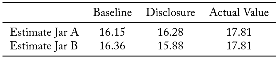
Figure 2. Boxplots of Incentivized Estimates and Actual Values

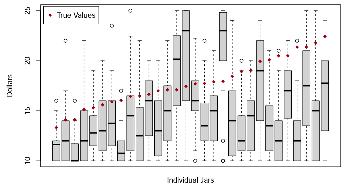
(Note: Subject guesses for each individual jar are displayed as separate boxplots. Plots are ordered by actual value of the jar. (Subjects did not see jars in value order.)

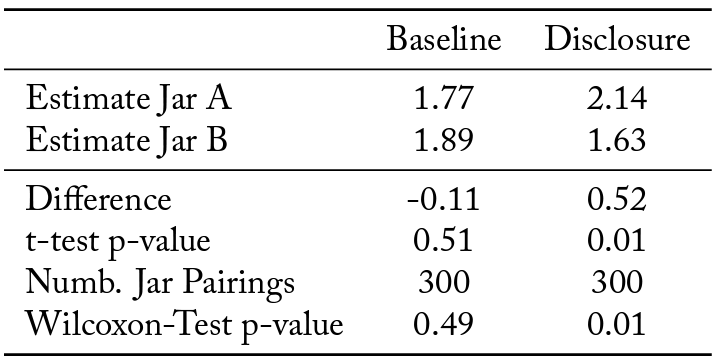
Table 3 reports similar information to Table 2, but it is presented as deviations from the average estimates in the Guess Experiment.¹⁰ Table 3 also reports the values from (two-sided) paired t-tests and Wilcox rank-sum tests comparing agent’s estimates when the jar is and is not bonus eligible (i.e., comparing estimates for a given image when that image is used as Jar A and Jar B, respectively). In the Baseline, the reported values for a given jar do not depend on whether the jar is Jar A or Jar B as the difference in estimates is not statistically different from zero. This result indicates that agents are not systematically favoring the bonus eligible jar in the Baseline. That is, when the conflict of interest is not disclosed there is no observed bias on the part of agents in the presence of reputation concerns. However, in the Disclosure Treatment, the difference is statistically significant with agents reporting higher estimates for a jar when it is the bonus earning Jar A than when it is the non-bonus earning Jar B. This indicates that disclosure of the conflict of interest introduces bias into agent estimation despite the presence of reputation concerns. To further analyze agent behavior we rely upon the following regression equation:

(2) $\begin{equation*} \hat{v}_{ijt}=\beta_{0}+\beta_{1}Value_{jt}+\beta_{2}Basline&JarA_{j}+\beta_{3}Disclosure&JarA_{j}+\beta_{4}Disclosure&JarB_{j}+\varepsilon_{ijt} \end{equation*}$

where $\hat{v}_{i j t}$ is agent $i$ ’s reported estimate of the value of jar $j$ in round $t$ . $\text { Value }_{j t}$ is a variable that captures the value of the coins in the jar for which the agent is providing an estimate. For robustness, we consider both the case where Value is the actual value of the coins in the jar (using the variable $\text { Actual Value }$ ) and the case where Value is the mean guess of the value of the coins in the jar from the Guess Experiment (using the variable $\text { MeanGuess }$ ). The main independent variables of interest are the interaction variables: $\text {Baseline & Jar A }$ , $\text {Disclosure & Jar A }$ , and $\text {Disclosure & Jar B }$ , which are all binary variables that take the value 1 if the estimate is for the stated jar in the stated condition and take the value 0 otherwise. The omitted group is $\text {Baseline & Jar B }$ , which serves as a reference point.

Table 3. Deviations from Guess Treatment Estimates for Cases in which each Jar was both A and B

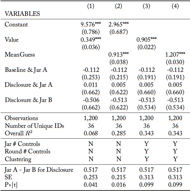
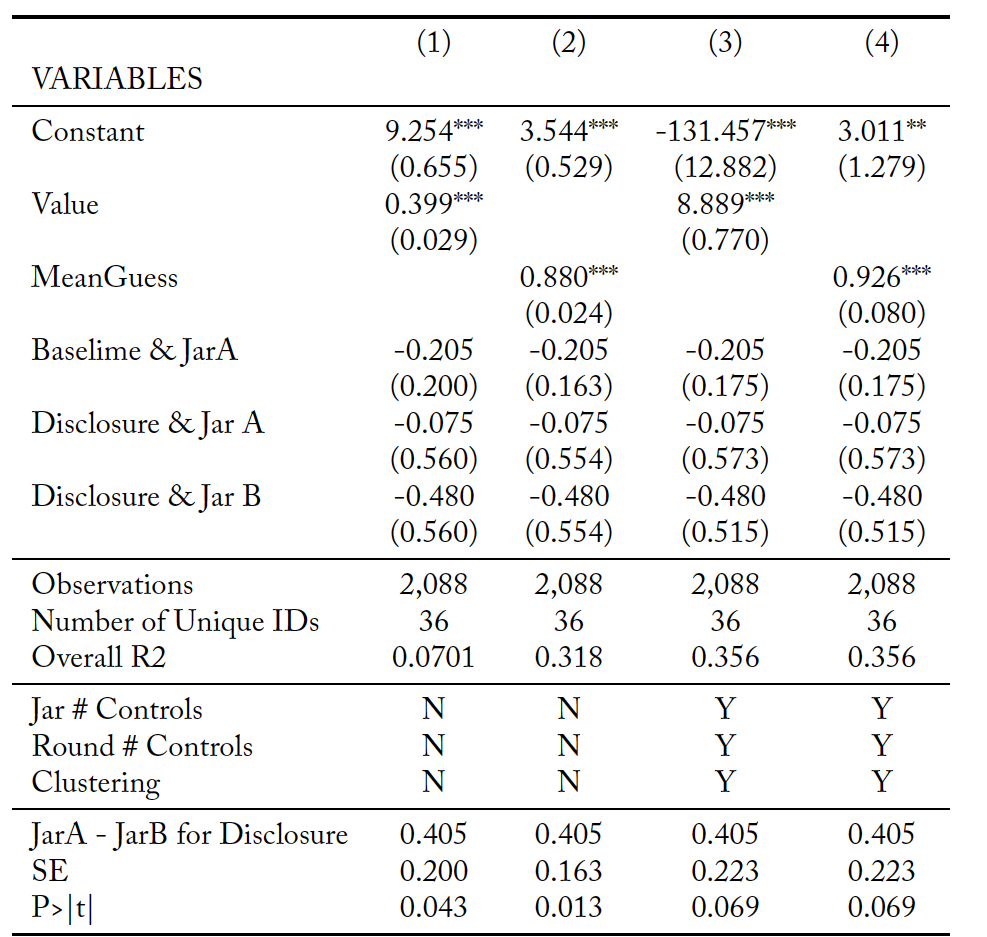
The regression estimation for agent reports is reported in Table 4. Specifications (1) and (3) use $\text {ActualValue}$ while specifications (2) and (4) use $\text {MeanGuess }$ . Specifications (1) and (2) do not include controls for the specific jars or round within a block nor do they cluster errors by agent, while specifications (3) and (4) do. We report all four specifications for the sake of robustness. The coefficient estimate for $\text {Baseline & Jar A }$ is not statistically significant in any specification. In fact, it is nominally negative, indicating the mean Jar A reported estimates are, if anything, less than the mean Jar B reported estimates. This pattern provides further evidence that in the absence of disclosure agents do not provide self-serving biased estimates systematically favor Jar A. However, as shown in the lower panel, which reports the estimated difference between $\beta_3$ and $\beta_4$ , in the Disclosure Treatment agents report that a jar is worth 51.7¢ more when it is Jar A than when it is Jar B. In all four specifications, this difference is positive and at least marginally statistically significant. Thus, when the conflict of interest is disclosed to principals then agents do provide self-serving estimates of jar value. Together, the evidence in Table 3 and Table 4 support Finding 2.

Finding 2A: In the absence of disclosure, agents do not exhibit bias when there are reputation concerns.

Finding 2B: In the presence of reputation concerns, disclosure of agents’ conflict of interest leads to biased and self-serving behavior.

In terms of the model by Levitt and List (2007) discussed in the previous section, the observed behavior indicates that agents believe disclosure creates a moral license to be self-serving and will reduce the scrutiny given to agent’s selfish action.

Table 4. Regression Estimates for Agents’ Estimates of Jars

Standard errors in parentheses. *** p<0.01, ** p<0.05, * p<0.1

3.3 Behavior of Principals

Principals make three sequential decisions each round: selecting an agent, choosing a jar based on the selected agent’s estimates, and rating the agent. In this subsection we analyze these three activities in turn.

Selecting an Agent

To examine how reputation impacts a principal’s selection of an agent, we estimate the following probit model:

(3) $\begin{equation*} Agent2_{it}=\Phi(\beta_{0}+\beta_{1}StarsDiff_{it}+\beta_{2}Disclosure_{i}*StarsDiff_{it}+\varepsilon_{ijt}) \end{equation*}$

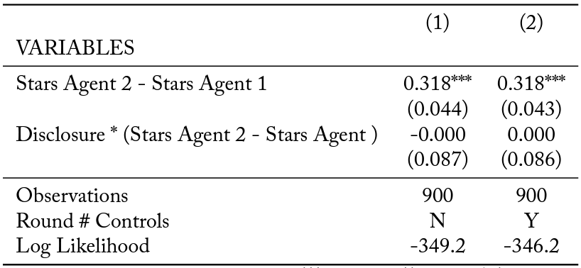
where $\text {Agent}2_{it}$ takes the value 1 if principal $i$ chose Agent 2 in round $t$ and the value 0 if Agent 1 was chosen. The independent variable, $\text {StarsDiff }$ , is the difference in the number of stars each agent has (i.e., Agent 2’s rating – Agent 1’s rating) for the two agents in the principal’s group in the given round. $\text {StarsDiff }$ is interacted with a binary variable for the Disclosure Treatment to allow for the rating differential to matter differentially to principals across treatments. The regression clusters standard errors at the principal level and includes a random effect for each principal.

Table 5 reports marginal effects from the estimation. Specifications (1) and (2) differ in that specification (2) includes controls for the specific round within the block while specification (1) does not. The estimation shows that each additional star in an agent’s rating over and above the rating of the other agent increases the likelihood of the higher-rated agent being selected by about 32%. Interestingly, the coefficient estimate for the interaction term is indistinguishable from zero, meaning that principals do not evaluate reputations differentially across treatments. That principals are more likely to select the agent with the higher rating indicates that reputation does matter in this setting and that agents are under pressure to maintain a high rating relative to the other agents. This is stated as Finding 3.

Finding 3: Principals rely on the rating system when selecting an agent, and thus agents face reputation concerns in this setting. However, the importance of reputation does not vary with disclosure of the agent’s conflict of interest.

Table 5. Estimated Marginal Effects of Likelihood of Choosing Agent 2

Standard errors in parentheses. *** p<0.01, ** p<0.05, * p<0.1

Choosing a Jar

Similar to the approach we use for identifying which agent a principal selects, we rely on a probit model to determine what influences the jar a principal selects. Specifically, we rely upon the following specification:

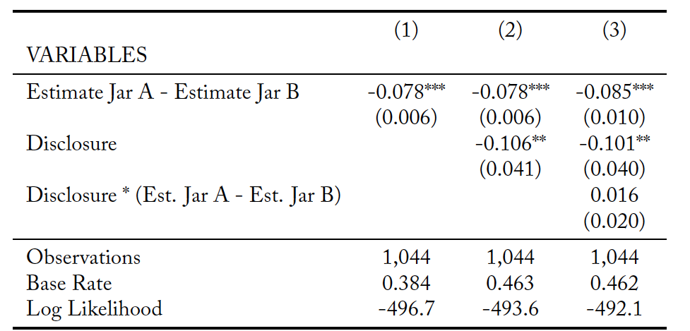
(4) $\begin{equation*} JarB_{it}=\Phi(\beta_{0}+\beta_{1}EstimateDiff+\beta_{2}Disclosure_{i}+\beta_{3}Disclosure_{i}*EstimateDiff_{it}+\varepsilon_{it}) \end{equation*}$

where $\text { JarB } _{it}$ indicates principal $i$ chose Jar B in round $t$ . The independent variable of interest is $\text {EstimateDiff }$ , which is the difference in the selected agent’s estimate of Jar A minus the selected agent’s estimate of Jar B. The regression includes a random effect for each principal and clusters standard errors by principal. Table 6 reports estimated marginal effects from the probit regression. In specification (1) it is assumed that there is no difference in jar selection between treatments, while specification (2) allows for the difference in jar selection to vary between treatments. The $\text {Disclosure }$ variable tests to see if the variation is significant. Specification (3) allows for a shift in jar selection due to the treatment. It also includes an interaction term between the treatment and $\text {EstimateDiff }$ .

The interpretation of the marginal effect of $\text {EstimateDiff }$ is that for every dollar that the estimate of Jar A exceeds Jar B there is a 7% decrease in the chance that Jar B is picked. The negative sign on this coefficient (in all specifications) is what one would expect if principals believe agent estimations convey useful information. From specifications (2) and (3), principals in the Disclosure Treatment are actually less likely to choose Jar B by 12% as compared to the Baseline, ceteris paribus. This effect is the opposite of what one would observe if principals were wary of choosing Jar A in the Disclosure Treatment, but it is consistent with principals not fully appreciating the implications of the agent’s conflict of interest and having a desire to help the agents earn a larger profit. Specification (3) reveals that the impact of differences in the reported estimated values of the jars does not vary with treatment. This leads to Finding 4.

Finding 4: Subjects directly rely on the agents’ estimates of jar value to determine which option to select in both treatments. However, Disclosure actually increases the likelihood that the principal will select the option that benefits the agent ceteris paribus.

Table 6. Estimated Marginal Effects of Likelihood of Choosing Jar B

Table 6

Standard errors in parentheses. *** p<0.01, ** p<0.05, * p<0.1

Rating the Agent

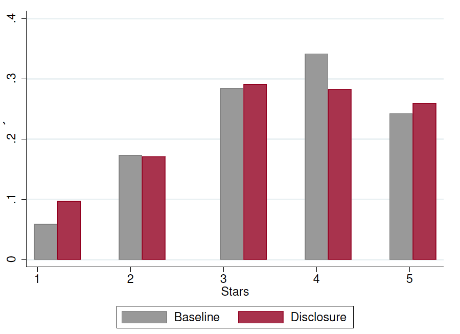
Figure 3 plots how often each star rating was assigned by treatment. The mean number of stars in the Disclosure Treatment (3.397) was slightly lower than the mean in the Baseline (3.487), but the difference is not statistically significant (p-value = 0.226).

Figure 3. Histogram of Stars (Ratings) of Agents

To understand how agent performance impacts the rating a principal gives an agent after observing the true value of the selected jar and the independent noisy signal of the value of the other jar, we rely on the two following specifications. The first specification classifies jars based on whether the agent had a conflict of interest with the jar or not (i.e., Jar A versus Jar B).

(5) $\begin{equation*} Stars_{it}=\beta_{0}+\beta_{1}AccurateDirection_{it}+\beta_{2}OverEstJarA_{it}+\beta_{3}UnderEstJarA_{it}+\beta_{4}OverEstJarb_{it}+\beta_{5}UnderEstJarB_{it}+\varepsilon_{it} \end{equation*}$

where $\text {Stars }_{it}$ is the number of stars principal $i$ assigned the selected agent in round $t$ . $\text {AccurateDirection }$ is a binary variable indicating that the jar the agent reported as having the highest value also had the highest value based upon the information subsequently revealed to the principal. That is, AccurateDirection takes the value 1 if the agent provided guidance to the principal that was in the “Accurate Direction” and is 0 otherwise. The remaining variables pertain to the difference between the agent’s estimate of a jar’s value and the subsequent information received by the principal. $\text {OverEstJarX }$ is the amount the principal believes the agent overestimated the value of Jar X while UnderEstJarX is the amount the principal believes the agent underestimated the value of Jar X. The second specification classifies jars based on whether the principal selected the jar or not.

(6) $\begin{equation*} Stars_{it}=\beta_{0}+\beta_{1}AccurateDirection_{it}+\beta_{2}OverEstPick_{it}+\beta_{3}UnderEstPick_{it}+\beta_{4}OverEstOther_{it}+\beta_{5}UnderEstOther_{it}+\varepsilon_{it} \end{equation*}$

where, similarly to Equation 1, $\text {OverEstPick (UnderEstPick, OverEstOther, UnderEstOther }$ ) denotes the amount by which the principal believes the agent over- (under-, over-, under-) estimated the value of the selected (selected, not selected, not selected) jar, respectively. This approach allows for the possibility that principals view errors asymmetrically. For both equations 1 and 2 we report 3 estimations. The first is just the basic specification given above. The second specification includes $\text {Disclosure }$ , a binary variable for the Disclosure Treatment, as well as the interaction of $\text {Disclosure }$ and $\text {AccurateDirection }$ . The third specification adds interaction terms for the type of error an agent made and the treatment to allow for the possibility that overestimation and underestimation are viewed differently between treatments.

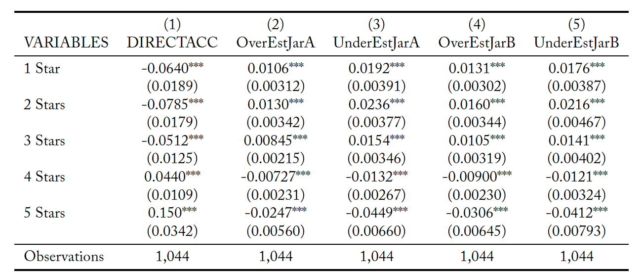
Table 7 reports regression estimates using Equation 1 and Table 8 reports regression estimates using Equation 2. In all three specifications in both tables, the coefficient on $\text {AccurateDirection }$ is positive and statistically significant, meaning that principals rate agents higher when the agent’s rank order Jars in a manner consistent with the independent information the principal receives. From all three specifications in both Tables 7 and 8 it is clear that agents are penalized for errors in their estimation. Specifications (2) and (3) in both tables indicate that ratings are not systematically different across treatments ( $\text {AccurateDirection & Disclosure }$ is not significant in any specification). The lower panel of both tables provides the p-values for testing for symmetry among the types of errors that an agent could make in her estimations. For each case there are six possible tests since there are four coefficients for over- and underestimation.¹¹

From Table 7 there is no evidence that overestimation of Jar A is treated differently than overestimation of Jar B, nor is underestimation viewed differently between jars. However, underestimation of a jar is viewed more negatively than overestimation of the same jar, although this difference is not always statistically significant across specifications and treatments. Interestingly, greater concern for underestimation as compared to overestimation holds across jars as well, at least for the Baseline. However, in the Disclosure Treatment when the principal knows the agent has an incentive to make Jar A appear more attractive, this cross-jar asymmetry disappears. That is, in the Disclosure Treatment, the principal views overestimating Jar A the same as underestimating Jar B as these two errors both make Jar A appear more attractive.

Unsurprisingly, Table 8 shows that overestimation of the jar selected is viewed more negatively than underestimation of the jar selected. Additionally, overestimation of the jar selected is viewed more negatively than overestimation of the jar not selected, which is intuitive. Overall, errors regarding the jar selected are viewed more negatively than oppositely signed errors for the non-selected jar. Thus, overestimation of the selected jar leads to a greater reduction in rating than does underestimating the value of the non-selected jar even though both errors have the same impact on assessing the difference in value between the two jars. But this asymmetry is limited to the Baseline as indicated by the tests of specification (3).

The results reported in Tables 7 and 8 support the final finding.

Finding 5: Principals reward agents with higher ratings when the agent appears to correctly identify the best option and punish agents with lower ratings for misestimation. The reduction in rating tends to be greater for underestimation than overestimation of a given jar; however, with Disclosure principals view overestimating one jar and underestimating the other jar as comparable. After selecting a jar, principals are more strongly concerned with errors regarding the selected jar; but, with Disclosure principals view overestimation of the selected jar as being comparable to underestimation of the other jar.

Table 7. Estimated Impacts on Ratings Given to Agent using Jar Identity

Table 7

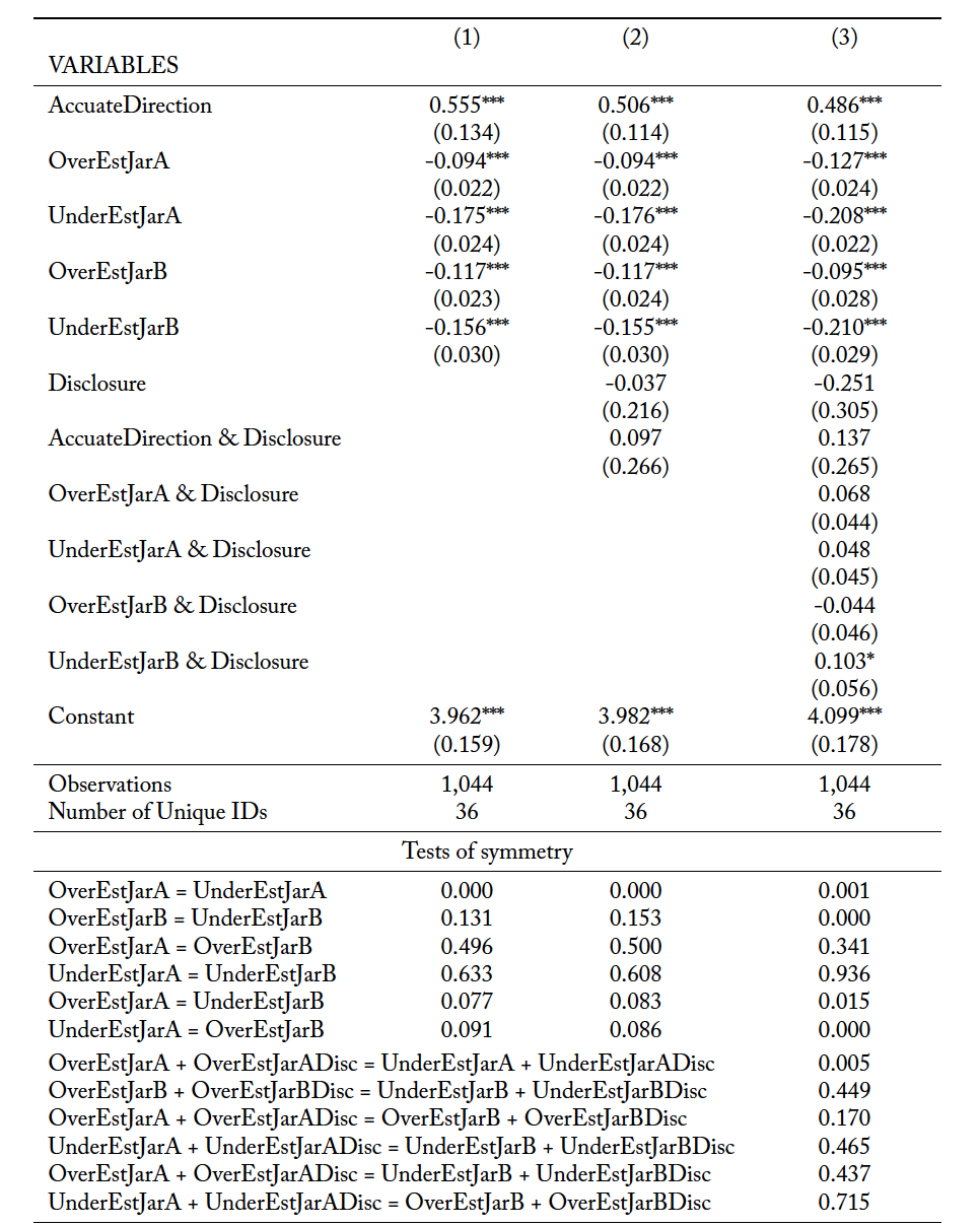
The results in the first four rows of specification (3) examine symmetry in the baseline and the last four test rows of specification test for symmetry in Disclosure.
Robust standard errors in parentheses. *** p<0.01, ** p<0.05, * p<0.1

Table 8. Estimated Impacts on Rating Given to Agent using Jar Selection

Table 8

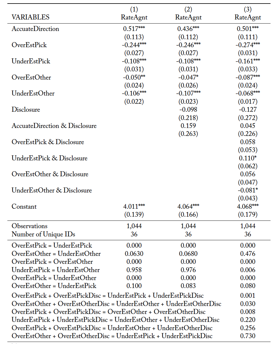
The results in the first four rows for specification (3) examine symmetry in the baseline and the last four test rows of specification test for symmetry in Disclosure.
Robust standard errors in parentheses. *** p<0.01, ** p<0.05, * p<0.1

4 Discussion

Conventional wisdom suggests that an agent’s conflict of interest should be disclosed to principals. However, such an policy may prove harmful if disclosure creates a moral license that emboldens agents and encourages them to act in self-serving ways, especially if the magnitude of this effect is not fully appreciated by principals. This negative effect was reported in Cain et al. (2005). Our paper extends the basic structure of Cain et al. (2005) to a repeated interaction situation in which agents have reputation concerns. The goal of our paper is two-fold. First, we seek to understand if the disciplining effect of maintaining a reputation can offset the incentives created by a conflict of interest. Second, we examine the effect of disclosure in a setting where agents have reputation concerns.

In our experimental task, principals rated agents based on the agent’s performance estimating the value of options available to the principal. In turn, principals could select agents based upon those ratings. Agents had a conflict of interest in that they received a direct benefit from increasing the principals belief about the relative value of a particular option. In the absence of disclosure, agents did not provide self-serving biased estimates. This indicates that reputation concerns alone can be enough to offset conflicts of interest. However, when disclosure of the conflict of interest was required, self-serving behavior on the part of agents was observed. The observed manipulation involved a mix of inflating estimates of the option that provided a benefit to the agent and deflating the estimate of the other option. Thus, we find that the counterintuitive result of Cain et al. (2005) that disclosure can exacerbate a conflict of interest holds even in the presence of reputation concerns.

While not the main focus of our study, the observed behavior does provide some additional insights. First, we find that misestimation of an option, whether it is ultimately the one selected or not, leads to a reduction in the rating a principal assigns to an agent. However, in the Baseline overestimating the benefit from a selected option leads to a greater reduction in the rating than underestimating the value of an option not selected, despite these errors having similar implications for the principal. But in the Disclosure Treatment principals view the two errors similarly.

Second, we find no evidence that with disclosure principals punish agents for self-serving estimates. In particular, disclosure does not lead to differences in how over- or underestimation of a particular option is treated. Finally, we note that our subjects were unable to accurately guess the value of the options, which were jars of coins, in a separate experiment used to calibrate unbiased expectations of those values. Instead, average estimates were systematically below the actual values, contrary to the arguments in Surowiecki (2005).

It is worth noting that the success of reputation concerns in deterring self-serving behavior by agents may be dependent upon two key features of our setting. First, principals in our study were effectively consuming a credence good since they could not verify the quality of their choice. However, the principals did receive a noisy signal of the quality. Second, the size of the conflict of interest was relatively small, in that a majority of the agent’s earnings were from being selected by a principal rather than having the principal select a particular choice. Whether a conflict of interest would lead to self-serving behavior when reputation concerns are present but either or both of these features is relaxed remains an important question. Similarly, the negative effects of disclosure that we observe may or may not hold as these two factors are relaxed. It is certainly possible that principals who know that agents have a substantial conflict of interest or who have weaker signals of agent performance may behave differently. We hope that our work will spark interest in these important avenues for future research.

Appendices

A.1 Instructions

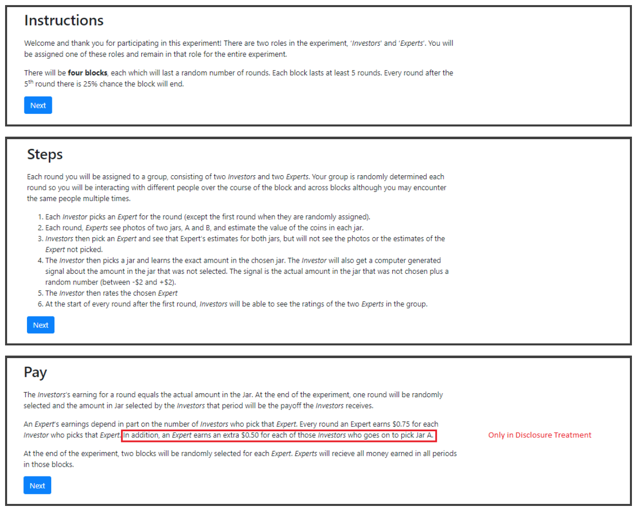
The experiment instructions were computerized, but subjects were informed that they could raise their hand if they had any questions. Screenshots of instructions are below.

Guess Treatment

The Guess Treatment had two instruction screens.

Main Treatments

The main treatments had four instruction screens with conditional text. Annotation shows what text was conditional on treatment.

A.2 Programming Error

In Round 1, agents saw Jars 1 and 2; for Agent 1 Jar 1 was Jar A and Jar 2 was Jar B, vice versa for Agent 2. In Round 2, agents saw Jars 3 and 4, assigned to A and B as above. Rounds continued like this until Round 15. In Round 15, agents saw Jars 1 and 2 a second time, with the assignment to A and B reversed. For Agent 2 Jar 1 was Jar A and Jar 2 was Jar B. This reversal occurred in Rounds 16 – 28 as well with each round being a swap of the round 14 rounds earlier. However, in round 29, the last given the random termination, Agents saw Jar 29 and Jar 30, which they had not seen before. Because of the odd number of rounds not every jar was observed twice.

Had every subject always been Agent 1 or always been Agent 2, every agent would have two estimates for each jar (1 to 28); one when the jar was Jar A and one when it was Jar B. However, there was an error in the logic of our program. A subject who was Agent 1 in the first half (e.g., Round 1) of the experiment could be Agent 2 14 rounds later (e.g., Round 15). As a result, while we have two estimates for each jar from 1-28 from each agent, for some agents some jars were estimates twice as Jar A and for others the jars were estimated twice as Jar B. For the analysis in the body of the paper, we only included estimates for which there were Jar A and Jar B estimates for the same jar by the same agent. Table A.1 reports estimates from repeating the regressions in Table 4 including all the estimates. The results are qualitatively similar. In the Baseline, guesses for the value of Jar B are larger than those for Jar A, but not by a statistically significant margin. In contrast, in the Disclosure Treatment, the guesses for the value of Jar A were 41¢ higher than those for Jar B.

Table A.1. KEEP ALL Regression Estimates for Agents’ Estimates of Jars

Standard errors in parentheses. *** p<0.01, ** p<0.05, * p<0.1

A.3 Ordered Probit Regressions

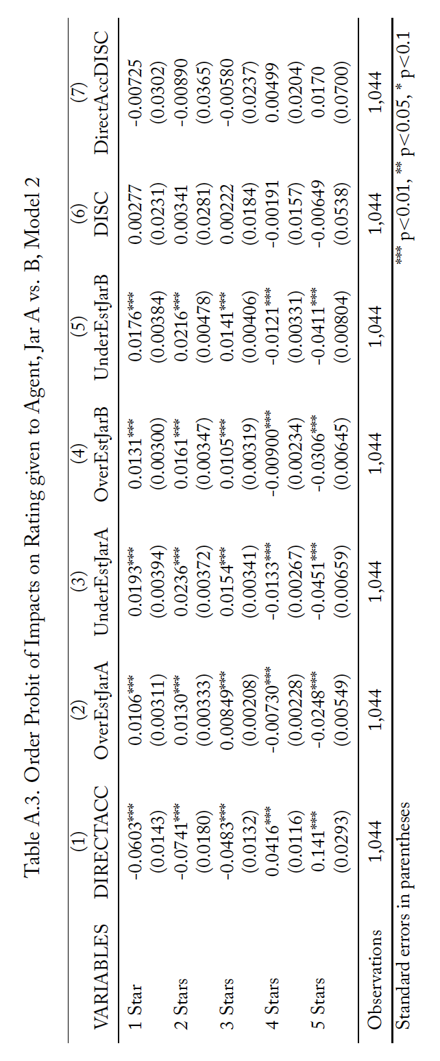
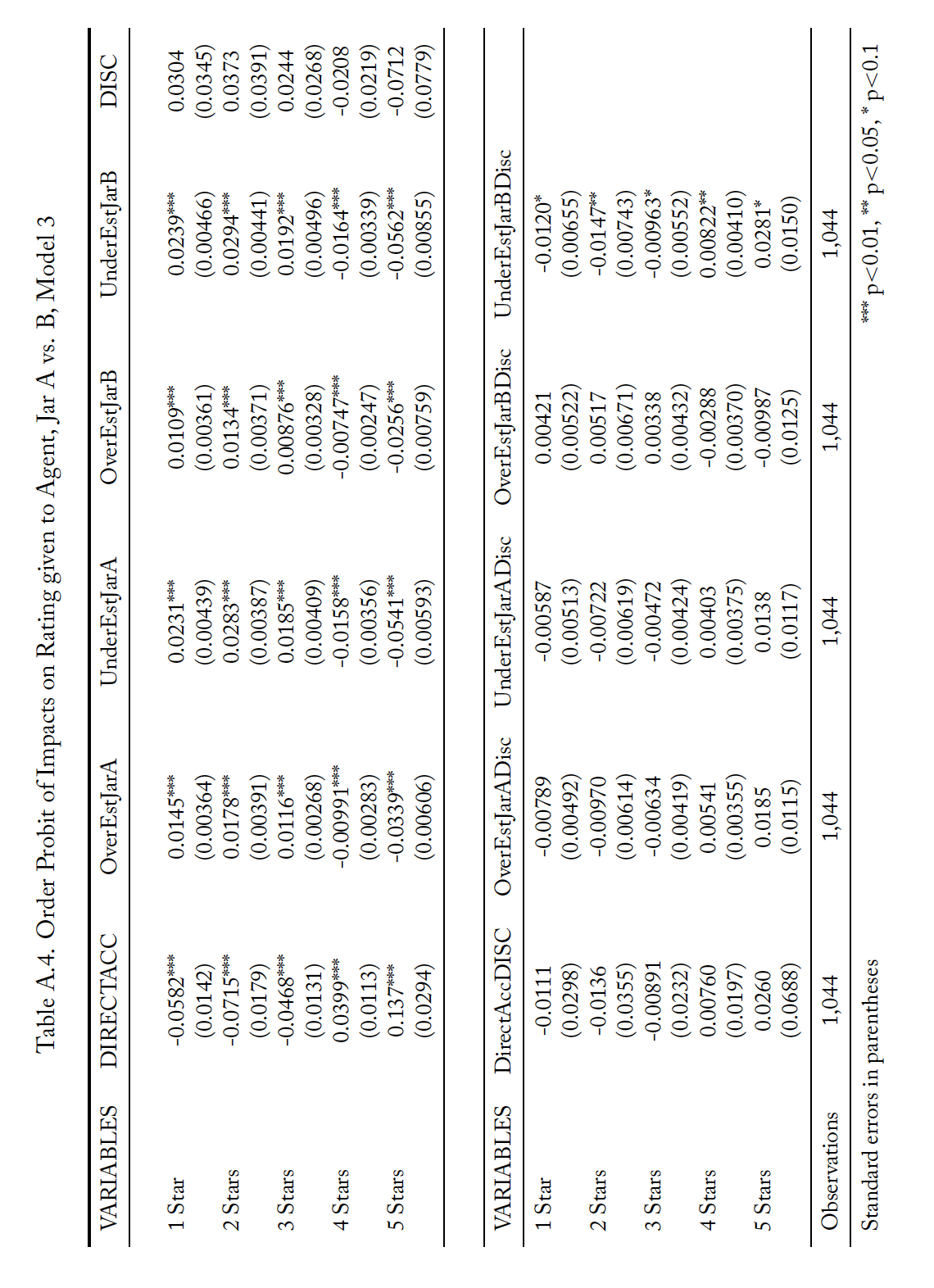
Tables A.2 through A.4 present results from analysis complementary to that reported in Table 7. However, rather than treating the number of stars awarded to an agent as a continuous variable, this supplementary analysis treats the ratings as discrete ranked options and thus uses ordered probit regressions. Each table reports the marginal effects of the probit regression in parallel to one of the specifications in Table 8. For these tables, each column is the effect from a single independent variable and each row is the change in the likelihood of an agent receiving that number of stars for a one unit change in the variable. The results are consistent with those from Table 8.

Table A.2. Order Probit of Impacts on Rating given to Agent, Jar A vs. B, Model 1

Standard errors in parentheses. *** p<0.01, ** p<0.05, * p<0.1

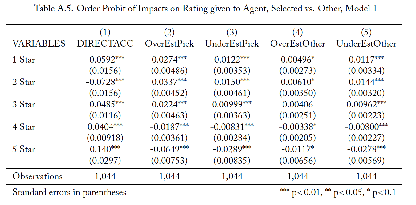
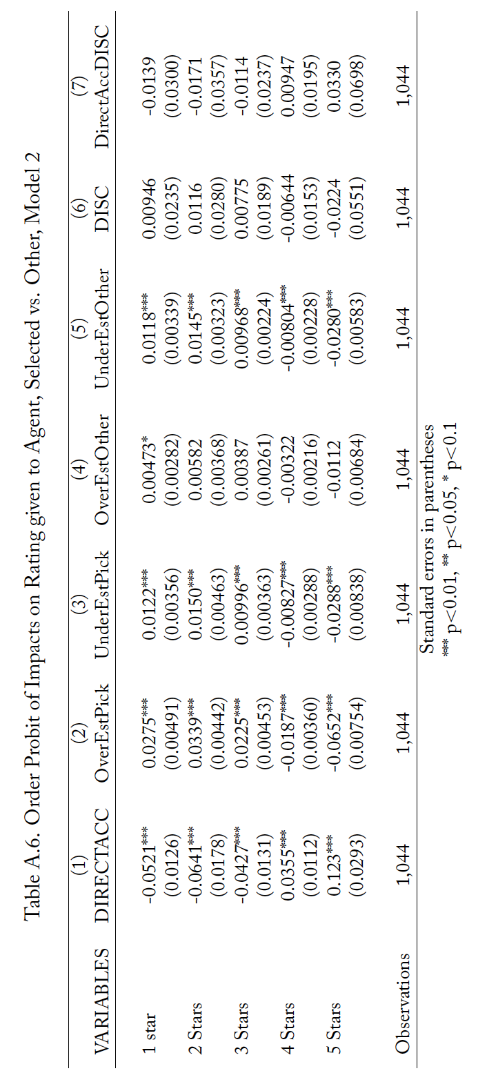
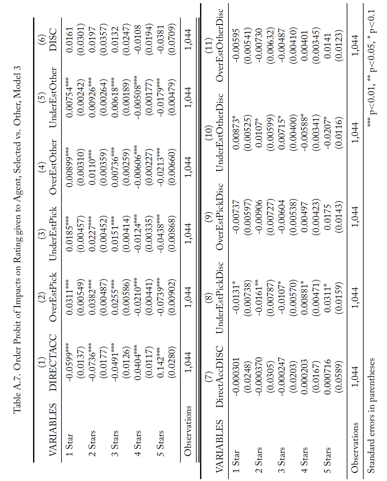
Tables A.5 through A.7 present results from analysis complementary to that reported in Table 8. However, rather than treating the number of stars awarded to an agent as a continuous variable, this supplementary analysis treats the ratings as discrete ranked options and thus uses ordered probit regressions. Each table reports the marginal effects of the probit regression in parallel to one of the specifications in Table 8. For these tables, each column is the effects from a single independent variable and each row is the change in the likelihood of an agent receiving that number of stars for a one unit change in the variable. The results are consistent with those from Table 8.

References

Becker, G. S. (1968). Crime and Punishment: An Economic Approach. Journal of Political Economy, 76(2):169. Ben-shahar, O. and Schneider, C. E. (2011). The Failure of Mandated Disclosure. University of Pennsylvania Law

Review, 159(3):647. Publisher: University of Pennsylvania Law School.

Boatright, J. R. (2000a). Conflicts of Interest in Financial Services. Business and Society Review, 105(2):201–219. _eprint: https://onlinelibrary.wiley.com/doi/pdf/10.1111/0045-3609.00078.

Boatright, J. R. (2000b). Ethics and the Conduct of Business. Prentice Hall, Upper Saddle River, NJ, 3rd edition.

Cain, D. M., Loewenstein, G., and Moore, D. A. (2005). The Dirt on Coming Clean: Perverse Effects of Disclosing Conflicts of Interest. Journal of Legal Studies, 34(1):1–25.

Campbell, E. G., Gruen, R. L., Mountford, J., Miller, L. G., Cleary, P. D., and Blumenthal, D. (2007). A National Survey of Physician–Industry Relationships. New England Journal of Medicine, 356(17):1742–1750. Publisher: Massachusetts Medical Society _eprint: https://doi.org/10.1056/NEJMsa064508.

Carl, W. J. (2008). The Role of Disclosure in Organized Word-of-Mouth Marketing Programs. Journal of Marketing Communications, 14(3):225–241. Publisher: Routledge.

Chen, D. L., Levonyan, V., Reinhart, S. E., and Taksler, G. (2019). Mandatory Disclosure: Theory and Evidence from Industry-Physician Relationships. Journal of Legal Studies, 48(2):409–440.

Chen, D. L., Schonger, M., and Wickens, C. (2016). oTree—An Open-Source Platform for Laboratory, Online, and Field Experiments. Journal of Behavioral and Experimental Finance, 9:88–97.

Darby, M. R. and Karni, E. (1973). Free Competition and the Optimal Amount of Fraud. Journal of Law and Economics, 16(1):67–88.

Dranove, D., Kessler, D., McClellan, M., and Satterthwaite, M. (2003). Is More Information Better? The Effects of “Report Cards” on Health Care Providers. Journal of Political Economy, 111(3):555. Publisher: The University of Chicago Press.

Gibbons, R. V., Landry, F. J., Blouch, D. L., Jones, D. L., Williams, F. K., Lucey, C. R., and Kroenke, K. (1998). A Comparison of Physicians’ and Patients’ Attitudes Toward Pharmaceutical Industry Gifts. Journal of General Internal Medicine, 13(3):151–154.

Grande, D., Shea, J. A., and Armstrong, K. (2012). Pharmaceutical Industry Gifts to Physicians: Patient Beliefs and Trust in Physicians and the Health Care System. Journal of General Internal Medicine, 27(3):274–279.

Green, M. J., Masters, R., James, B., Simmons, B., and Lehman, E. (2012). Do Gifts From the Pharmaceutical Industry Affect Trust in Physicians? Family Medicine, 44(5):7.

Guo, T. and Sriram, S. (2017). “Let the Sun Shine In”: The Impact of Industry Payment Disclosure on Physician Prescription Behavior. SSRN Electronic Journal.

Guo, T., Sriram, S., and Manchanda, P. (2017). The Effect of Information Disclosure on Industry Payments to Physicians. SSRN Electronic Journal.

Hannan, E. L., Kilburn, H., Racz, M., Shields, E., and Chassin, M. R. (1994). Improving the Outcomes of Coronary Artery Bypass Surgery in New York State. JAMA, 271(10):761–766. Publisher: American Medical Association.

Kerschbamer, R. and Sutter, M. (2017). The Economics of Credence Goods–-A Survey of Recent Lab and Field Experiments. CESifo Economic Studies, 63(1):1–23.

Levitt, S. D. and List, J. A. (2007). What Do Laboratory Experiments Measuring Social Preferences Reveal about the Real World? Journal of Economic Perspectives, 21(2):153–174.

Mainous, A. G. (1995). Patient Perceptions of Physician Acceptance of Gifts from the Pharmaceutical Industry. Archives of Family Medicine, 4(4):335–339.

Mukamel, D. B. and Mushlin, A. I. (1998). Quality of Care Information Makes a Difference: An Analysis of Market Share and Price Changes after Publication of the New York State Cardiac Surgery Mortality Reports. Medical Care, 36(7):945–954. Publisher: Lippincott Williams & Wilkins.

Pope, D. G. (2009). Reacting to Rankings: Evidence from “America’s Best Hospitals”. Journal of Health Economics, 28(6):1154–1165.

Rose, S. L., Sah, S., Dweik, R., Schmidt, C., Mercer, M., Mitchum, A., Kattan, M., Karafa, M., and Robertson, C. (2019). Patient Responses to Physician Disclosures of Industry Conflicts of Interest: A Randomized Field Experiment. Organizational Behavior and Human Decision Processes.

Scholl, B. and Hung, A. A. (2018). The Retail Market for Investment Advice. Technical report, Secuity and Exchange Commission, Washington, D.C.

Surowiecki, J. (2005). The Wisdom of Crowds. Anchor Books, New York, 1st Anchor Books edition. OCLC: 61254310.

Wolinsky, A. (1993). Competition in a Market for Informed Experts’ Services. RAND Journal of Economics, 24(3):380–398.

Keeping a Clean Reputation: More Evidence on the Perverse Effects of Disclosure

Executive Summary

Resources

Focuses

1 Introduction

2 Experimental Design and Hypotheses