
Introduction
A transportation system provides mobility for people living in a community. It allows businesses to move goods cheaply, increasing economic activity. An efficient transportation system promotes better matches between jobs and workers, which increases labor productivity. Mobility depends on the physical capacity of the transportation infrastructure and any resulting congestion. As economic activity expands, congestion becomes a more significant factor influencing mobility.1 Robert Krol, “Transportation, Mobility, and Economic Growth,” InsideSources, January 19, 2017.
Highway congestion is a costly problem in urban areas. The two most common policy approaches to reducing congestion are to expand highway capacity and to build mass-transit systems. Because both responses are expensive and have a poor track record when it comes to reducing congestion, many economists have proposed that it would be more efficient for policy makers to focus on road pricing. Variable tolls on all or some highway lanes can manage traffic flows.2Robert Krol, “Tolling the Freeway: Congestion Pricing and the Economics of Managing Traffic” (Mercatus Research, Mercatus Center at George Mason University, Arlington, VA, 2016).
What is the best approach for public officials who wish to promote or maintain high levels of mobility? The basic policy question centers on whether expanding highway capacity is the most efficient way to manage congestion. Would demand management (i.e., tolling) be a better alternative?
As economist Anthony Downs has pointed out, expanding highway capacity does not fully eliminate congestion.3Anthony Downs, “The Law of Peak-Hour Expressway Congestion,” Traffic Quarterly 16 (1962): 393–409; Anthony Downs, Stuck in Traffic: Coping with Peak-Hour Traffic Congestion (Washington, DC: Brookings Institution, 1992); Anthony Downs, “Traffic: Why It’s Getting Worse, What Governments Can Do” (Policy Brief, Brookings Institution, Washington, DC, 2004). The additional highway capacity draws more vehicles to the road. In the economics literature, this behavior is known as induced travel (or induced demand), sometimes called the fundamental law of congestion.4 Gilles Duranton and Matthew A. Turner, “The Fundamental Law of Road Congestion: Evidence from U.S. Cities,” American Economic Review 101, no. 6 (2011): 2616–52. Induced travel is a broader measure than induced demand, signifying the increase in vehicle miles traveled that results from an increase in highway capacity. Induced travel includes a wider set of behavioral responses to additional highway lanes. Most empirical studies are measuring induced travel. The difference is discussed in more detail later in the paper.
Ultimately, the issue boils down to quantity: How much travel is induced? This is an empirical question. It turns out that estimating the amount of induced travel is complicated; researchers have taken different approaches. This paper critically reviews the evidence found in the economics literature. The best-structured empirical studies find that induced travel is economically significant, reducing the congestion relief benefits from highway expansion.
Because highway expansion is costly, especially in urban areas, the presence of significant induced travel suggests that highway demand management using tolls may be a more efficient policy approach to reduce congestion in urban areas. This does not mean that cities should never expand highway capacity. Clearly, rapidly growing cities will require expanded highway capacity. However, one important advantage of having a tolling system in place is that driver responses to tolls send a clear signal to transportation policy makers, indicating exactly where limited funds should be spent on incremental highway construction. This information can result in a better use of limited infrastructure funds.5Robert Krol, “Political Incentives and Transportation Funding” (Mercatus Research, Mercatus Center at George Mason University, Arlington, VA, 2015).
Congestion Trends
Congestion is getting worse in the United States. The Texas A&M Transportation Institute quantifies congestion in terms of time delays and the dollar value of those delays.6David Schrank et al., 2015 Urban Mobility Scorecard (Texas A&M Transportation Institute and INRIX Inc., 2015). Figures 1 and 2 show the congestion trends in terms of time delays and costs between 1996 and 2014.
Time delays have risen from 4.2 billion hours in 1996 to 6.9 billion hours in 2014. This represents a 64.3 percent increase. When the dollar values of the wasted time and fuel costs are added together, the dollar cost of congestion has risen from $93 billion in 1996 to $160 billion in 2014, a 72 percent increase. The only year-over-year decline occurred in 2009, a result of the severe recession that reduced driving. To put these numbers into practical terms, the institute’s report estimates that the average urban driver needs to allow 48 minutes for a rush-hour trip that would take 20 minutes on a congestion-free highway.7In a 2012 version of the report, the authors provide data on the percentage increase in congestion over time for groups of urban areas. Their chart suggests that areas that had greater increases in road capacity experienced smaller increases in congestion. This is a misleading interpretation of the data. Without controlling for population and economic growth, it is not possible to conclude that highway expansion is the cause of the decline in congestion. The authors of the report also caution readers that other factors may have contributed to the decline in congestion. David Schrank, Bill Eisele, and Tim Lomax, 2012 Urban Mobility Report (Texas A&M Transportation Institute, 2012).
Figure 1. Total US Congestion Time Delays, 1996–2014
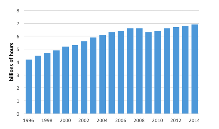
Source: David Schrank et al., 2015 Urban Mobility Scorecard (Texas A&M Transportation Institute and INRIX Inc., 2015).
Figure 2. Total US Costs of Congestion, 1996–2014
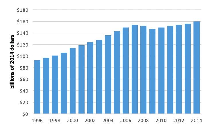
Source: David Schrank et al., 2015 Urban Mobility Scorecard (Texas A&M Transportation Institute and INRIX Inc., 2015).
Table 1 provides a rough picture of the demand and supply forces that drive rising congestion. Demand factors include the growth in the adult population, in registered vehicles, and in vehicle miles traveled. Highway supply is measured in terms of highway and road lane miles. The highway statistics are for major roads, a category that includes interstate highways, freeways, and principal arterial roads.8 These roads carry high traffic volumes and represent a major percentage of trips in urban areas.
For the US as a whole, the adult population, number of registered vehicles, and vehicle miles traveled increased twice as fast as the number of lane miles between 1996 and 2014. In urban areas, where lane miles have expanded more than 35 percent, which is more than 20 percentage points faster than in the country as a whole, highway expansion was still unable to keep up with the 45 percent increase in vehicle miles driven. These numbers suggest that while highway capacity has grown over the past 20 years, capacity has not kept pace with expanding travel.
Table 1. Factors Influencing US Congestion
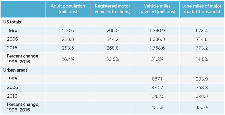
Sources: Federal Reserve Bank of St. Louis, “Population,” FRED, accessed January 26, 2019, https://fred.stlouisfed.org/categories/104; Registered Motor-Vehicles Table MV-1, Vehicle Miles Traveled Tables VM-2 and HM-44, and Lane-Miles of Major Roads Tables HM-20 and HM-60 from the 1996, 2006, and 2016 issues of Federal Highway Statistics, https://www.fhwa.dot.gov/policyinformation/statistics.cfm.
Note: Adult population is the civilian, noninstitutional population 16 years of age or older living in the US.
Economics of Induced Travel (Induced Demand)
A common policy approach to mitigate urban congestion is to add lanes to a city’s highways and roads. These changes in highway capacity initially reduce the time and gasoline costs of travel.9While the focus of this paper is on the impact of highway capacity on demand and congestion, other shifts in transportation policies—such as expansions of public transit or private-sector parking benefits—can have similar effects. This is discussed later in the paper. As a result, we expect to observe changes in travel behavior. The addition of lanes to a congested highway increases traffic speeds, thus lowering the price (or cost) of driving. As a result, more drivers choose to use the highway. Additional drivers on the highway represent the induced travel (induced demand) from highway capacity expansion.
The additional vehicles come from a number of sources. As highway capacity expands, individuals take more and longer trips.10 New trips represent what is called latent travel demand. Some public-transportation users switch back to using the more flexible car as a mode of transportation. Public transit systems may reduce the frequency of trips or raise fares as ridership declines, causing even more individuals to drive. These behavioral changes represent induced demand, which includes only new vehicle miles traveled as the result of an increase in highway capacity. Drivers who have planned trips at less optimal times may shift some trips to peak hours. Individuals who traveled on less-preferred routes may shift to the expanded highway. Other long-run adjustments may include an increase in car ownership or spatial reallocation of activities, such as the replacement of central business districts with regional malls and changes in residential locations.11 Robert B. Noland, “Relationships between Highway Capacity and Induced Vehicle Travel,” Transportation Research Part A: Policy and Practice 35 (2001): 47–72. All of these behavioral travel adjustments together represent the broadest measure called induced travel.
These behavioral changes can be easily understood using a simple supply and demand framework.12 Much of this analysis draws on two sources: Noland, “Relationships between Highway Capacity and Induced Vehicle Travel”; and Robert B. Noland and Lewison L. Lem, “A Review of the Evidence for Induced Travel and Changes in Transportation and Environmental Policy in the U.S. and U.K.,” Transportation Research Part D: Transport and Environment 7 (2002): 1–26. Figure 3 illustrates the induced travel effect on a congested highway when capacity expands.
Figure 3. Induced Travel Effect of a Highway Expansion
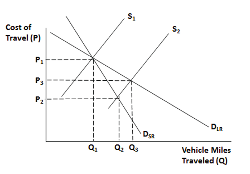
The vertical axis measures the price or cost of travel (P). This includes fuel costs, wear and tear on the vehicle, and the value of the commuter’s time. Variation in the time cost of travel is the key factor in this analysis. As congestion increases and highway speeds slow, travel time for the same trip increases. Because time has value in terms of forgone wages and leisure, the time cost of the trip increases as the travel time increases. The horizontal axis measures the quantity of travel (Q), measured in vehicle miles traveled.
The analysis includes a supply curve (S) that reflects the private cost of using the highway.13 The supply curve represents the private average cost of using the highway, or the cost per vehicle. The cost increases with vehicle miles traveled because speeds slow and hence travel time increases. Private costs are also a function of, or are conditional on, highway capacity. For uncongested highways, the supply curve would be flat to reflect constant travel costs. Also, when the highway is at capacity with total gridlock, the supply curve would be vertical. This analysis focuses on congested highways that have positive average speeds. This analysis does not include the external costs. See Noland, “Relationships between Highway Capacity and Induced Vehicle Travel”; Noland and Lem, “Review of the Evidence for Induced Travel”; Duranton and Turner, “Fundamental Law of Road Congestion”; Jan K. Brueckner, Lectures on Urban Economics (Cambridge, MA: MIT Press, 2011), chap. 5. Changes in highway capacity cause the supply curve to shift. In this example, the increase in highway capacity lowers the travel cost, causing the supply curve to shift to the right. Also included are short-run and long-run demand curves (DSR and DLR).14Here’s a brief explanation of the demand curve, as it applies to driving: Drivers choose between using the highway and using alternate travel routes and modes. If an individual chooses the highway, that means it is the low-cost route for that individual. In other words, it is cheaper than the alternate route. The demand curves measure drivers’ willingness to pay for using the highway. The most they are willing to pay for using the highway is an amount that equals the cost of using the alternate route. The cost of the alternate route or mode will vary by individual, depending on the individual’s spatial location. At the equilibrium level of vehicle miles traveled, willingness to pay represented by the height of the demand curve equals private average cost represented by the height of the supply curve. See Kenneth A. Small and Erik T. Verhoef, The Economics of Urban Transportation (New York: Routledge, 2007); Duranton and Turner, “Fundamental Law of Road Congestion”; Brueckner, Lectures on Urban Economics. Economic growth and demographic trends can cause the demand curve to shift. We initially hold these other factors constant, which determines the location of the demand curve. The long-run demand curve is shown to be relatively more price elastic (i.e., the long-run demand curve shows a greater response to price changes than the short-run demand curve), because the behavioral adjustments from a price change should be larger over time (in the long run), as drivers have more time to adjust. For example, highway expansion can cause people to change where they live, causing an increase in traffic volume over time (in the long run).
Price P1 and quantity Q1 represent the initial congested highway’s equilibrium. When highway capacity is expanded, the supply curve shifts from S1 to S2 , lowering the cost of using the highway. This results in a new short-run equilibrium at price P2 and quantity Q2 . The change in quantity demanded from Q1 to Q2 represents the short-run induced travel (induced demand) from highway expansion. The behavioral adjustment of travelers resulting from the lower travel cost is larger in the long run. This can be observed by examining the adjustment along the long-run demand curve. In this case, the induced long-run quantity demanded equals the change from Q1 to Q3.15As will be discussed later, the empirical research finds larger changes in the long-run than in the short-run adjustment. Because the traffic volume is larger and speeds are lower as time passes and people have time to adjust, the price of traveling on the highway is higher at the new long-run equilibrium (P3) than at the new short-run equilibrium (P2).
The previous analysis held economic growth, population growth, and other demographic factors constant. When these factors change, the demand curve shifts. When researchers estimate the induced travel associated with highway expansion, they must control for these factors that impact traffic volume independently of road expansion. This is illustrated in figure 4.
Figure 4. Highway Expansion Accompanied by Economic Growth
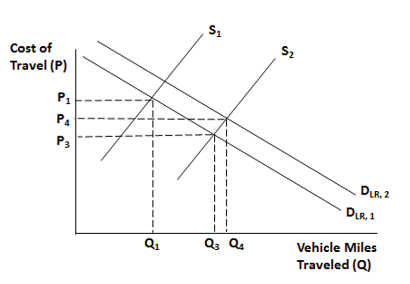
Figure 4 is much like figure 3, except that the analysis only uses a long-run demand curve. The initial equilibrium is at price P1, quantity Q1 . The figure also shows the long-run equilibrium price P3 and quantity Q3 from figure 3. The same highway capacity expansion is captured by shifting the supply curve from S1 to S2 , as in figure 3. However, in this case, simultaneous economic growth causes the demand curve to shift from DLR, 1 to DLR, 2. The long-run equilibrium occurs at price P4 and quantity Q4 . While the total change in vehicle miles traveled on the highway equals Q4 minus Q1 , the induced quantity demanded from highway capacity expansion equals the smaller quantity Q3 minus Q1 . The difference Q4 minus Q3 represents the additional vehicle miles traveled on the highway owing to economic growth. Researchers must control for the growth in demand factors that increases vehicle miles traveled on a highway, or they will overstate the size of the induced quantity demanded.
Empirical Issues and Evidence
Issues
Economists and transportation analysts have tried to estimate the magnitude of induced travel (induced demand) that results from a highway expansion. In a nutshell, they want to estimate the elasticity of vehicle miles traveled with respect to greater highway capacity (i.e., the percent change in vehicle miles traveled divided by the percent change in lane miles). Does it approximately equal one, or is it significantly less than one? If the elasticity equals one, expanding capacity does little to reduce congestion because for every 1 percent increase in lane miles, there is a 1 percent increase in vehicle miles traveled. If the elasticity is less than one, for every 1 percent increase in lane miles, there is less than a 1 percent increase in vehicle miles traveled. In this case, expanding highway capacity would lower congestion.
In the research literature, the standard empirical model used to estimate the elasticity of vehicle miles traveled with respect to lane miles regresses vehicle miles traveled on lane miles. In addition, control variables that measure demographic factors and economic activity that can influence vehicle miles traveled are also included in the model.16All variables are in logarithmic form, so estimated coefficients can be interpreted as an elasticity
Including either lagged vehicle miles traveled or lane miles in the regression analysis enables the model to better capture longer-run dynamic adjustments. It is reasonable to assume that the behavioral adjustment that results from expanding the highway does not occur quickly; including lagged behavioral variables captures the gradual adjustment of driving behavior and land-use patterns.
There are a number of issues that make estimating the induced travel (induced demand) effect difficult. The omission of important variables that influence vehicle miles traveled causes an “omitted variable bias” that results in a biased elasticity estimate.17 When the omitted variable that influences vehicle miles traveled is correlated with other explanatory variables in the regression, the estimated impact coefficient of the explanatory variable will be biased. In order to address this problem, researchers expand the data used in the analysis by incorporating more explanatory control variables. The most reliable studies use panel data in the empirical analysis. Panel data include observations across highways, cities, or states (observational units) over a period of years. In contrast, cross-sectional studies examine data across highways, cities, or states only at a point in time.
Panel data have a number of advantages. The increased number of observations allows the researcher to include more control variables and still get precise estimates of key parameters. Since not all factors that influence vehicle miles traveled are observable, when these variables differ across observational units but not over time, panel data estimates can include what are called “fixed effects.”18 See James H. Stock and Mark W. Watson, Introduction to Econometrics (Boston: Addison-Wesley, 2015); Jeffrey M. Wooldridge, Econometric Analysis of Cross Section and Panel Data (Boston: MIT Press, 2010). For example, the geographic terrain can vary between observational units but not change over time. Fixed effects are indicator variables (dummy variables) that take on the value one for a particular observational unit, but equal zero for other observational units.19 These dummy variables effectively adjust the regression intercept term for fixed unobserved differences between observational units. Panel data models can also adjust for “time effects.” If an unobserved variable differs over time but not across observational units, say the business cycle, a dummy variable for each time period is included in the model.
The direction of causality is another issue. In the case of estimating induced travel from highway expansion, does population growth and an increase in vehicle miles traveled drive the need to increase capacity, or does increasing capacity causes greater vehicle miles traveled? When this question is not addressed, standard econometric estimation methods (ordinary least squares) provide biased results.
An instrumental-variable estimation technique can be used to handle this problem. This involves a twostage estimation process. When highway capacity is influenced by vehicle miles traveled, the researcher must find variables (instrumental variables) that are correlated with highway capacity, but do not affect vehicle miles traveled. For example, as one of its instrumental variables for actual urban interstate lane kilometers, one study used metropolitan statistical area (MSA) highway kilometers from the 1947 interstate highway plan. These are highly correlated with actual urban interstate highways built, but are not affected by current vehicle miles traveled.20 Duranton and Turner, “Fundamental Law of Road Congestion.” Highway capacity is then regressed on the instrumental variable or variables. The predicted value from this regression for highway capacity, instead of actual highway capacity, is used to estimate the impact of highway capacity on vehicle miles traveled. This method provides statistically consistent results.21 See Stock and Watson, Introduction to Econometrics, chap. 10. However, without good instruments, using an instrumental variables technique can produce more biased estimates. Good instruments—variables that result in a high correlation with the actual variables—allow for more meaningful hypothesis testing.22 John Bound, David A. Jaeger, and Regina M. Baker, “Problems with Instrumental Variables Estimation When the Correlation between the Instruments and the Endogenous Explanatory Variables Is Weak,” Journal of the American Statistical Association 90 (1995): 443–50; Isaiah Andrews, James Stock, and Liyang Sun, “Weak Instruments in IV Regression: Theory and Practice” (unpublished manuscript, August 2, 2018), PDF file.
Finally, as more time passes following a highway expansion, the behavioral adjustment tends to be larger. As a result, the estimated short-run elasticity of vehicle miles traveled with respect to the number of lane miles is likely to be smaller than the long-run elasticity. This can be taken into account by including lagged values of vehicle miles traveled in the regression.23 See William H. Greene, Econometric Analysis, 2nd ed. (New York: Macmillan, 1993), chap. 18
Evidence
This section includes results from key studies that have empirically examined the relationship between highway capacity and vehicle miles traveled. Only panel data studies are included, because they provide more reliable results.
The size of the estimated induced travel varies across studies. This variation occurs because there is significant variation among studies in model specification and data used. Studies use alternative estimation methods, including standard ordinary least squares, fixed effects, and instrumental variables. The control variables and instrumental variables vary among studies. Table 2 summarizes the results of the panel data studies.24 This review focuses on the papers that best handle the econometric problems in this research area.
Table 2. Summary of Key Elasticity Estimates25Note: MSA = metropolitan statistical area. VMT = vehicle miles traveled. a Exact years vary by state. Years 1985–95 include all states; Maryland spans 1969–96, North Carolina 1985–97, Virginia 1970–96, and DC 1970–96. b Total road lane miles and vehicle miles traveled are broken down among interstate, arterial, and collector roads. c An important difference in this paper is that the author estimates the models using disaggregated data simultaneously using the seemingly unrelated regression method. This approach assumes that the error terms from each type of road classification regression are correlated. This results in a more precise estimate. See William H. Greene, Econometric Analysis, 2nd ed. (New York: Macmillan, 1993), chap. 17. d They include MSA interstate highway kilometers from the 1947 highway plan, MSA railroad routes in 1898, and the exploration routes between 1835 and 1850.
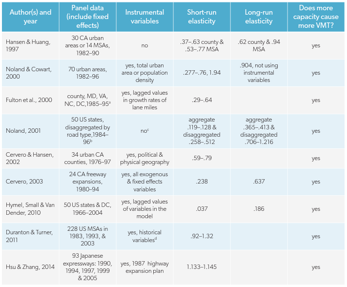
Sources: Mark Hansen and Yuanlin Huang26, “Road Supply and Traffic in California Urban Areas,” Transportation Research Part A: Policy and Practice 31, no. 3 (1997): 205–18; Robert B. Noland and William A. Cowart, “Analysis of Metropolitan Highway Capacity and the Growth in Vehicle Miles of Travel,” Transportation 27, no. 4 (2000): 363–90; Lewis M. Fulton et al., “A Statistical Analysis of Induced Travel Effects in the Mid-Atlantic Region,” Journal of Transportation and Statistics 3, no. 1 (2000): 1–30; Robert B. Noland, “Relationships between Highway Capacity and Induced Vehicle Travel,” Transportation Research Part A: Policy and Practice 35 (2001): 47–72; Robert Cervero and Mark Hansen, “Induced Travel Demand and Induced Road Investment: A Simultaneous Equation Analysis,” Journal of Transport Economics and Policy 36, no. 3 (2002): 469–90; Robert Cervero, “Road Expansion, Urban Growth, and Induced Travel,” Journal of the American Planning Association 69, no. 2 (2003): 145–63; Kent M. Hymel, Kenneth A. Small, and Kurt Van Dender, “Induced Demand and Rebound Effects in Road Transport,” Transportation Research Part B: Methodological 44 (2010): 1220–41; Gilles Duranton and Matthew A. Turner, “The Fundamental Law of Road Congestion: Evidence from U.S. Cities,” American Economic Review 101, no. 6 (2011): 2616–52; Wen-Tai Hsu and Hongliang Zhang, “The Fundamental Law of Highway Congestion Revisited: Evidence from National Expressways in Japan,” Journal of Urban Economics 81 (2014): 65–76.
A number of conclusions can be drawn from the results reported in table 2. First, there is clear evidence that expanding highway capacity results in greater vehicle miles traveled (induced travel). The estimated elasticity of vehicle miles traveled with respect to highway capacity is positive and significant. Some of the estimates suggest it does not differ significantly from one, which would mean that adding capacity does not reduce congestion. There is also evidence that higher vehicle miles traveled result in increases in lane miles, an example of reverse causality.27 Robert Cervero and Mark Hansen found that the elasticity of lane miles with respect to vehicle miles traveled was between .33 and .79. Robert Cervero and Mark Hansen, “Induced Travel Demand and Induced Road Investment: A Simultaneous Equation Analysis,” Journal of Transport Economics and Policy 36, no. 3 (2002): 469–90. This result illustrates why using instrumental variables estimation is important in getting meaningful empirical results.
Adding lanes to congested highways is unlikely to dramatically reduce congestion. Highway traffic volume will increase, which does provide benefits to residents using the highway, but congestion will likely remain. This conclusion follows from the fact that many of the long-run estimates of the elasticity of vehicle miles traveled with respect to lane miles are close to one.28Mark Hansen and Yuanlin Huang, “Road Supply and Traffic in California Urban Areas,” Transportation Research Part A: Policy and Practice 31, no. 3 (1997): 205–18; Robert B. Noland and William A. Cowart, “Analysis of Metropolitan Highway Capacity and the Growth in Vehicle Miles of Travel,” Transportation 27, no. 4 (2000): 363–90; Noland, “Relationships between Highway Capacity and Induced Vehicle Travel”; Duranton and Turner, “Fundamental Law of Road Congestion”; Wen-Tai Hsu and Hongliang Zhang, “The Fundamental Law of Highway Congestion Revisited: Evidence from National Expressways in Japan,” Journal of Urban Economics 81 (2014): 65–76. However, an elasticity value of one is not a universal result from the research literature.
Second, there is a wide range of estimates on the size of induced travel. This is the case because researchers use different units of observation, study different geographic areas or particular highways, examine different time periods, employ different model specifications (control variables), and adopt different estimation methods.
Differences in the unit of observation can be important. For example, when state data are used, some behavioral changes, such as drivers switching to an expanded road, do not show up in the data. The increase in vehicle miles traveled on the expanded highway is offset or “netted out” by the decline in vehicle miles traveled on a previous route driven. In this setting, increases in vehicle miles traveled reflect only induced demand, from new or longer trips. We would expect the size of the elasticity of vehicle miles traveled with respect to increased lane miles to understate the actual response. Alternatively, studies that examine specific highways capture the broader measure of induced travel, which also includes drivers shifting routes and changes in the timing of trips. The magnitude of the response would be expected to be larger in this case.29Robert Cervero, “Road Expansion, Urban Growth, and Induced Travel,” Journal of the American Planning Association 69, no. 2 (2003): 145– 63; Duranton and Turner, “Fundamental Law of Road Congestion”; Hsu and Zhang, “Fundamental Law of Highway Congestion Revisited.”
Third, as one would expect, the long-run increase in vehicle miles traveled as a result of greater highway capacity is larger than the short-run adjustment.30This conclusion is consistent with Phil B. Goodwin’s synthesis of the earlier literature on induced travel. Goodwin concluded that the elasticity of traffic volume with respect to travel time was about −.5 in the short run and up to −1.0 in the long run. Phil B. Goodwin, “Empirical Evidence on Induced Demand: A Review and Synthesis,” Transportation 23, no. 1 (1996): 35–54. This result is not surprising because, as more time passes, behavioral adjustments are greater. People relocate and land-use patterns change as a result of highway expansion.31Hansen and Huang, “Road Supply and Traffic in California Urban Areas”; Noland and Cowart, “Analysis of Metropolitan Highway Capacity”; Noland, “Relationships between Highway Capacity and Induced Vehicle Travel”; Cervero, “Road Expansion, Urban Growth, and Induced Travel.”
Fourth, most of the studies use the expansion of lane miles as the force that lowers the cost of traveling on a highway. If expanding capacity on a highway with little congestion does not lower driving costs, the estimates of the impact of highway construction on congestion will be small and of little value. One study uses the increase in average recorded travel speeds to measure the cost of driving on a highway—a better measure than lane capacity.32Cervero, “Road Expansion, Urban Growth, and Induced Travel.” In this case, the elasticity measures the percent change in vehicle miles traveled in response to a percent change in average highway speed.
The 2003, 2011, and 2014 studies provide the strongest results.33 Cervero, “Road Expansion, Urban Growth, and Induced Travel”; Duranton and Turner, “Fundamental Law of Road Congestion”; Hsu and Zhang, “Fundamental Law of Highway Congestion Revisited.” But each has drawbacks. The advantage of Robert Cervero’s 2003 paper is that he uses highway speed, rather than lane miles, in his analysis. As I pointed out earlier, additional lane miles on uncongested highways will not result in faster speeds and quicker trips. This implies that lane miles may not always cause travel costs to decline. However, Cervero does not report statistics about the quality of the instrumental variables used in his study. So it is unclear whether his estimates satisfactorily resolve the simultaneous relationship between vehicle miles traveled and highway capacity.
Both the 2011 study by Gilles Duranton and Matthew A. Turner and the 2014 study by Wen-Tai Hsu and Hongliang Zhang use highway lane kilometers rather than speed. However, since their focus is on congested urban areas where adding lanes will surely reduce congestion initially, this should not have much of an impact on their results. But, since they use total vehicle kilometers traveled as the dependent variable, it becomes more difficult to identify the source of the increase traffic volume, new trips versus changes in the timing of trips, resulting from highway expansion.
Duranton and Turner’s paper is worth looking at in greater detail. The authors analyzed a large sample of 228 interstates and highways located in urban MSAs over time.34 The years were 1983, 1993, and 2003. Duranton and Turner, “Fundamental Law of Road Congestion.” They used planned interstate highway kilometers from the 1947 highway plan, MSA railroad route kilometers from 1898, and the routes taken by explorers during the first half of the 19th century as their instrumental variables for actual lane kilometers. All three of these variables are highly correlated with the actual routes of interstate highways built, but are not closely related to current vehicle miles traveled, controlling for population.35Duranton and Turner report test statistics showing that these instrumental variables have high explanatory power over lane miles. This is one of the few studies that reports test statistics. Duranton and Turner, “Fundamental Law of Road Congestion.” A possible drawback of using these instrumental variables is that they are better predictors of the initial building of the interstate highways than of the later addition of lanes. This is a weakness in Duranton and Turner’s analysis. Still, the high predictive content from these variables suggests that this is not a serious problem.
Duranton and Turner found the elasticity of vehicle miles traveled with respect to lane kilometers to be around one. In other words, congestion returned because of induced travel (induced demand). Many of their elasticity estimates did not differ significantly from one. These results are higher than the results reported in much of the previous literature on this topic.
Interestingly, Duranton and Turner found that public transit, as measured by major heavily used bus routes, does not impact the results. They also found that expanding highways results in a large increase in long-haul truck traffic. Their estimates show that expanding lanes increases individual driving and population. They found little evidence that traffic is being diverted from other roads. For example, they found that a 10 percent increase in urban interstate highway capacity results in a decline of about 0.5 percent in vehicle kilometers traveled on major urban roads. This suggests that, while there is some substitution between alternative roads, the magnitude is modest.36Duranton and Turner, “Fundamental Law of Road Congestion.”
Hsu and Zhang produce an analysis similar to that of Duranton and Turner of induced travel for Japan. Following Duranton and Turner, Hsu and Zhang use planned highways taken from the 1987 highway report for Japan as instrumental variables for lane kilometers for major highways in Japan. Once again, these plans are highly correlated with actual highway expansion but are not affected by current vehicle miles traveled in Japan. They find elasticity estimates greater than one. This suggests what the authors call a coverage effect. The coverage effect refers to a situation where additional or longer highways expand the areas serviced by the road, causing a more-than-proportional increase in trips. Hsu and Zhang find this to be the case in Japan.37Hsu and Zhang, “Fundamental Law of Highway Congestion Revisited.”
Other Policy Options
Given the findings of the empirical literature, that highway expansion induces travel, one has to conclude that adding new lanes to highways will not necessarily provide the desired relief in terms of congestion. Other than Cervero’s short-run estimate, the literature suggests that induced travel is fairly large, more than .6 or .7.
To answer the question posed in the title of this paper, it is difficult to build sufficient infrastructure in dense urban areas so as to significantly reduce congestion. This does not mean that growing urban areas do not benefit from expanding highway capacity—but this capacity is unlikely to solve serious congestion problems in the long run. It is worth examining other policies that can be directed at reducing urban congestion.
Expanding Fixed-Rail Public Transit
Fixed-rail public transit is not a substitute for highway construction, nor does it show potential for reducing congestion except in the most densely populated communities. Mass transit is very costly, so it only makes sense if it will be heavily used.38 Rhiannon Jerch, Matthew E. Kahn, and Shanjun Li, “The Efficiency of Local Government: The Role of Privatization and Public Sector Unions,” Journal of Public Economics 154 (2017): 95–121. The costs of mass transit can be justified in densely populated cities where the majority of jobs (and shopping outlets) are concentrated in or near a central business district. This is a reasonable description of New York, but cities that grew in the post–World War II automobile era are not dense enough. In these communities, jobs, shopping, and residences are decentralized, making fixed rail ineffective as a predominant transportation mode.39 In newer, decentralized cities, buses are a less expensive and more flexible means of providing public transit. Randal O’Toole, Gridlock: Why We’re Stuck in Traffic and What to Do about It (Washington, DC: Cato Institute, 2009); Randal O’Toole, “The Coming Transit Apocalypse” (Policy Analysis #824, Cato Institute, Washington, DC, 2017). Additional expansion of fixed-rail systems would only be successful if, at the same time, incentives were established to return business to the inner city. Flat or declining ridership trends indicate that commuters do not find public transit to be an attractive option.40 O’Toole, Gridlock; O’Toole, “Coming Transit Apocalypse.”
Furthermore, expanding fixed-rail transit is likely to suffer an induced travel problem similar to that of added highway capacity. If expanding fixed-rail transit initially resulted in a shift of commuters from cars to rail, highway congestion would decline and highway speeds increase, reducing the cost of driving. This reduction in driving costs would, over time, attract more drivers, as in the case of highway construction, eliminating some of the gains associated with the initial reduction in congestion. How big these travel adjustments would be depends on the community, its residents, and the substitutability of one means of commuting for another. The evidence on the impact of fixed-rail expansion on highway congestion is inconclusive. One problem is that researchers often fail to control for other factors that influence travel choices. Researchers have not quantified the long-run compared to the short-run impact of fixed-rail expansion on congestion.41 For a discussion of the evidence, see Molly D. Castelazo and Thomas A. Garrett, “Light Rail: Boom or Boondoggle?,” Regional Economist (Federal Reserve Bank of St. Louis), July 2004; Nathaniel Baum-Snow and Matthew E. Kahn, “Effects of Urban Rail Transit Expansions: Evidence from Sixteen Cities, 1970–2000,” Brookings-Wharton Papers on Urban Affairs, 2005, 147–206; Duranton and Turner, “Fundamental Law of Road Congestion”; Todd Litman, “Critique of ‘Transit Utilization and Traffic Congestion: Is There a Connection?,’” Victoria Transport Policy Institute, 2014. Nathaniel Baum-Snow and Matthew E. Kahn find that most of the mode-of-travel changes are between buses and rail, not cars and rail. This would weaken the congestion relief effects of public transit.
The basic question concerning fixed-rail public transit is whether the benefits of rail (reduced congestion and pollution) outweigh construction and maintenance costs. In their 2007 study, Clifford Winston and Vikram Maheshri examined 25 transit systems in the US. They calculated the net benefits of these systems, including any reductions in congestion.42 They do not take into account environmental effects. Clifford Winston and Vikram Maheshri, “On the Social Desirability of Urban Rail Transit Systems,” Journal of Urban Economics 62, no. 3 (2007): 362–82. For the year 2000, they estimated that costs outweighed benefits in all cases except that of the BART system in San Francisco. They conclude that, in general, transit systems do not raise social welfare owing to their high operating and capital costs and low ridership.43Winston and Maheshri, “On the Social Desirability of Urban Rail Transit Systems.” Christopher Severen finds this to be the case for Los Angeles using more recent data. Christopher Severen, “Commuting, Labor, and Housing Market Effects of Mass Transportation: Welfare and Identification” (Working Paper 18-14, Federal Reserve Bank of Philadelphia, 2018). Molly D. Castelazo and Thomas A. Garrett draw the same conclusion for St. Louis. Castelazo and Garrett, “Light Rail.”
Congestion Pricing
If expanding highway capacity and building fixed-rail transit systems are weak options for solving urban congestion problems, what is the alternative? Most economists point out that the fundamental cause of highway congestion or overuse is that we price highways incorrectly. Most US highways are toll free.44 There are some toll roads in the U.S. Some of these roads are private and in other situations they are tolled individual lanes that parallel tollfree highway lanes. This leads to overuse and congestion.
On a congested highway, each additional driver causes the average speed to decline, resulting in longer travel times. In effect, additional drivers impose a cost (an externality) on other drivers using the highway. The solution is to charge a toll equal to this external cost. In this case, tolls would be highest during peak rush-hour travel times and low during off-peak times. The high tolls during rush hours would create an incentive for some drivers, those with the most flexibility, to shift trip times away from peak hours, use alternate routes, carpool, or use existing public transit. This would lead to fewer cars on the highway and less congestion.45 Krol, “Tolling the Freeway.” It doesn’t take a large reduction in congestion to increase the traffic flow.
This pricing strategy is a common solution to peak demand problems in other industries. For example, airline ticket prices are higher during peak holiday travel times. It would not make economic sense for airlines to keep ticket prices constant and invest in more airplanes that would be idle much of the year.
During peak driving times, optimal tolls should be high enough to at least cover the marginal cost of using the highway. This includes the maintenance cost for the highway, plus pollution and congestion costs. During off-peak times, tolls should reflect only maintenance, construction, and pollution costs. Although it is not easy to quantify pollution and congestion costs, cities that have used variable tolls have had success in setting tolls that alleviate major congestion and gain popularity with drivers.
Tolls are politically unpopular. Voters see them as yet another tax. But tolls are one of the very few efficient taxes, because they don’t distort the relative prices of goods and they discourage the congestion externality.46 Krol, “Tolling the Freeway.” To increase political support for tolls, politicians might offer them as a replacement for fuel taxes.
A key, often unrecognized, benefit of tolling is that it produces information about which routes drivers value the most, identifying areas where additional highway investment would actually make economic (rather than political) sense. For example, evidence that rush-hour tolls must dramatically rise to control congestion on a highway segment is a signal that the drivers paying the tolls place a high value on the benefits of using the route. Given limited highway funding, expanding these highways would increase driver welfare the most. Tolling congested highways results in a more efficient use of limited highway space. In addition, with variable tolling in place, we might find out that we do not need to expand the transportation system as much as we thought. This would free limited tax revenue for other uses or allow reductions in other taxes.47 For further details about this topic, see Krol, “Tolling the Freeway.”
Compared to the traditional approach—adding highways and public transit—tolling highways is an efficient way to manage local infrastructure. States may toll new interstate highways or new lanes added to existing interstates, but federal law prohibits tolling on existing interstates. The federal government could encourage efficient infrastructure investment by eliminating any remaining federal restrictions on interstate tolls. Expanding tolling is a smart policy solution.48 Duranton and Turner note that expanding highway capacity and public transit capacity are ineffective policies for reducing congestion. They suggest using some form of tolling to reduce congestion. Duranton and Turner, “Fundamental Law of Road Congestion.” Educating voters and opening the interstates to tolling are the first steps.
Conclusions
Most highways in urban areas experience some degree of congestion, which reduces mobility, imposing substantial costs on drivers. Furthermore, data indicate that urban congestion is getting worse. In response, many cities have chosen to expand their highway infrastructure by building additional lanes (or fixed-rail transit lines). This is very expensive. Furthermore, expanded capacity attracts more drivers, making any congestion relief temporary or limited. This paper outlines the economics that spur this behavior—what economists call induced travel or induced demand—and reviews evidence about its magnitude.
When congested highways are expanded, driving speeds increase, at least temporarily, lowering the cost (time savings) to drivers using the highway. This lower cost results in changes in the behavior of commuters around the previously congested highway. Drivers take more trips. Some commuters who have been using alternate, less desirable, routes or public transit switch to the faster expanded highway. As a result, all or most of the congestion returns.
Induced travel is measured by estimating the elasticity of vehicle miles traveled with respect to lane miles. There is a wide range of estimates for this elasticity. Most estimates indicate a value significantly greater than zero. Some studies find that the value of the induced travel elasticity does not differ significantly from one. These results indicate that induced travel takes on an economically meaningful magnitude. While expanding highway capacity increases total traffic volume, which raises community welfare, it is unlikely to be an efficient solution to major highway congestion issues. One potential policy alternative would be to repeal or reduce fuel taxes and replace the lost revenues with a variable tolling system.