
Introduction
Wildlife vehicle collisions (WVCs) cause injuries and deaths in both humans and wildlife in areas where big game animals are abundant (Allen and McCullough, 1976; Conover et al., 1995; Bruinderink and Hazebroek, 1996; Bissonette et al., 2008; Cramer et al., 2022). Despite continuous efforts to mitigate WVCs with different types of mitigation measures, a significant amount of WVCs remain.1Several strategies, either alone or in combination, have been implemented to reduce WVCs, such as wildlife crossings, wildlife fencing, nighttime speed limits, and reflective warning signs (Clevenger et al., 2001; Huijser et al., 2016; K¨ammerle et al., 2017; Benten et al., 2018; Riginos et al., 2022; Caldwell and Klip, 2021). Collisions between big game animals and vehicles are frequently fatal, resulting in high societal costs (Huijser et al., 2009; Donalson and Elliott, 2020). Every year, reported WVCs kill over 200 and injure 26,000 people, costing more than $8 billion USD (Huijser et al., 2008), and it is estimated that the direct costs of wildlife vehicle collisions total nearly $50 million per year in Wyoming alone (Riginos et al., 2018). This issue concerns drivers and underscores the urgency to evaluate whether existing measures are effective and to what extent those measures provide protection against potentially fatal and financially costly events.
This paper examines the causal reduction of WVCs attributed to wildlife crossing structures (WSs),2This paper uses the term “wildlife crossing structure” when referring to the combination of wildlife crossing and fencing. which are widely regarded as the most effective in terms of reducing WVCs while connecting habitats (Huijser et al., 2016). Despite the large social impact of WVCs, few economic studies estimate the social costs and effectiveness of different crossing structures. Prior studies have concentrated on counting carcasses found alongside the road, relying on motion-activated cameras or GPS collars to track wildlife animals’ use of the crossings. However, these studies often overlook confounding effects, such as selection bias and time-variant and time-invariant, that inhibit the ability to draw causal conclusions to evaluate the cost-effectiveness of new investments in WVC mitigation measures(Huijser et al., 2009; Clevenger et al., 2001; McCollister and Manen, 2010; Huijser et al., 2016; Caldwell and Klip, 2021).
Because traditional proxies3For example, motion-activated cameras and GPS collars that record wildlife crossing the structure cannot provide evidence of reduced WVCs for several reasons. First, not every crossing would lead to a collision. Second, they cannot capture whether the wildlife crosses the road if there is no WS. Third, they also cannot capture whether the wildlife crosses the road more often when there is a safe passage provided. Many studies that count carcasses found alongside the road did not control for the placement of the WS. The WS placement is not a random event, as it is placed in a location where most WVCs are observed in the area. Comparing carcass counts in the WS area in the post-intervention period and its surrounding area overlooks the fact that the WS area is expected to experience more WVCs. On the other hand, comparing carcass counts in the WS area in the pre- and post-intervention period fails to account for the time-varying confounders. For example, there could be policy changes that affect how many carcasses that could be found alongside the road in the pre- and post-intervention period. In this study, I explain how reducing traffic volume due to COVID-19 could lead to a biased estimate. Further, many studies did not investigate whether there is a spillover effect, which can be positive or negative. The positive sources of spillover can come from increase in wildlife crossing at the end of the fences. Because there is fencing that prevents wildlife from crossing in the area, wildlife that do not find the overpass might cross at an unfenced area. This in turn creates another hotspot of WVCs. The negative spillover can come from wildlife learning about the WS and starting to use it every time they need to cross the road. These are a few examples of why traditional proxies and methodologies have not been adequately addressing the potential confound effects. for WVCs are likely to be biased, this study employs a novel data set containing high-resolution and officially documented WVC incidents together with a quasi-experimental econometric design.4A quasi-experimental design does not rely on the random assignment of the treatment effect to be able to establish a causal relationship. This study uses an econometric tool and a quasi-experimental design to overcome the nonrandomness in the treatment assignment and other potential time-varying and nonvarying confounders. In addition, given the natural experimental context, I use a difference-in-differences (DD) estimation with count data in the negative binomial distribution context to quantify the causal effect of WS on WVC reductions.5A DD estimation with Poisson distribution is performed as a robustness check and is presented in Appendix table A5. I further restrict observations in close proximity to the WS, with the assumption that the only difference between the controls and treatments is that controls do not receive the WS intervention, given the high spatial resolution and temporal nature of the data.6As robustness checks, analysis with all the observations on I-80 on the entire state of Utah are also included and presented in Appendix tables A3 and A4, respectively. The reduction effect most predominantly appears in deer vehicle collisions, which account for over 86 percent of all WVCs in the area.
I find evidence of a positive spillover of WVCs, yet the net social improvement of the WS is valued over $15 million USD over the lifetime of WS, with 77 percent directly benefiting the home state and 23 percent benefiting out-of-state resident. With the $5 million of the WS being federally funded and maintenance being state funded, the WS appears to be overly dependent on federal funding, which stalls the construction of new infrastructure that provides high value to society.
This study contributes by providing a comprehensive and rigorous economic analysis of the most effective measure in reducing WVCs and mitigating habitat fragmentation (i.e., the combination of wildlife crossing and fencing structures). Using a state-of-the-art causal inference approach, it overcomes endogeneity and overdispersion problems that are common in previous literature and uses high-resolution carcass data to evaluate the effectiveness of the WS. It also identifies and quantifies the positive spillover of WVCs due to the WS and explores the distribution of benefits to in- and out-of-state residents. Findings of this study can better inform policymakers when allocating funds effectively to promote roadway safety and biodiversity.
The rest of the paper proceeds as follows. Section 2 provides background information on the adaptation of WSs in the US and the study region. Section 3 describes my data, and Section 4 discusses the methods. Section 5 presents my empirical results and interprets the magnitude of the WVC reduction effect. Section 6 evaluates and discusses its policy implications, and Section 7 concludes.
Background
WSs have been implemented across the United States, especially in areas where rich wildlife resources intersect with busy interstates or highway traffic, contrary to the perception that WVCs only occur in rural areas (Western Transportation Knowledge Network, 2021). At the time of writing, several new major WSs are underway. These include wildlife crossings at Liberty Canyon on Highway 101 in California,7The Liberty Canyon overpass will be the world’s largest wildlife crossing, spanning across an eight-lane highway and costing $61.5 million (State of California, 2022). Castle Rock on Interstate 25 in Colorado, and Pigeon River Gorge on Interstate 40 in North Carolina. The pressing and increasing numbers of WVCs every year due to continuous urbanization and habitat fragmentation underscore the urgency to better understand the so-called most effective measure. Notably, the recent Infrastructure and Jobs Act allocated a $350 million fund dedicated for building WSs (Federal Highway Administration, 2021).
Utah’s Parleys Canyon overpass is one of the few recent WSs that combines a crossing structure and fencing on a busy US interstate. The canyon is located in northern Utah, where most WVCs have occurred in Utah. The Parleys Canyon overpass and fences, as shown in figure 1, are located at the epicenter of most WVCs in Utah. The overpass is constructed over the six-lane Interstate 80 near Parleys Summit, with 3.5-mile fences on both sides, and was completed in early December 2018 (Helean, 2022).
Figure 1. Density Map: WVCs in Utah, 2010–2021
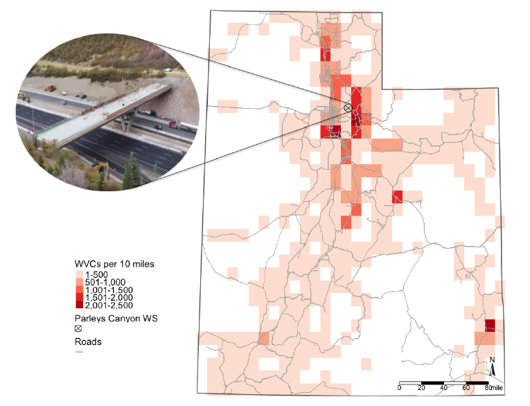
Note: WVC data from 2010 to 2021 are obtained from the Utah Department of Transportation and the Utah Division of Wildlife Resources. WVC density is derived from dividing by the number of WVCs in a 10×10 mile grid across the entire state of Utah over the 12-year study period. Photo credit: Utah Department of Transportation.
Table 1 reports the number of the top three big game animals whose carcasses are found on the side of the road in the study area from January 2010 to November 2021. Mule deer is the most common big game involved in WVCs and pose the greatest threat to the area. Moose and elk vehicle collisions, on the other hand, account for a much smaller proportion of collisions. Nevertheless, moose and elk are much larger in size and weight, and the damage they cause are reflected in their corresponding estimated average collision costs. The collision cost (table 1, column 3) used in this study is consistent with the Huijser et al. (2008) report to Congress. This report, in particular, estimates the average animal-specific collision cost using several studies on a wide span of geographical locations nationally and internationally.8Interested readers can refer to Huijser et al. (2008) (chapter 3) for additional information. The report breaks down and itemizes vehicle repair costs, human injuries, human fatalities, towing costs, accident attendance and investigation, monetary value of animals, and carcass removal and disposal per collision for each type of WVC. The calculation accounts for the likelihood of the different WVC severity levels.9From the nationwide data, WVC-induced fatality is 0.04 percent, severe injury is 0.5 percent, minor injury is 1.7 percent, possible injury is 2.3 percent, and no injury is 95.4 percent (Huijser et al., 2008). The nationwide average statistics closely resembles that in Utah. The corresponding WVC crash severity for Utah is 0.04 percent, 0.38 percent, 2.36 percent, 3.59 percent, and 93.62 percent. The associated cost of property damage only is $2,570, possible human injury is $24,418, evident human injury is $46,266, incapacitating/severe human injury is $231,332, and human fatality is $3,341,468, according to 1994 US Department of Transportation and corrected for the GDP deflator through the fourth quarter in 2006 (Huijser et al., 2008).
Data and Identification
All relevant wildlife collisions are attributed using spatially and temporally explicit data from the Utah Department of Transportation and the Utah Division of Wildlife Resources. The data range from January 2010 to November 2021 and include every carcass found and reported on the side of the road throughout the state on a daily and per carcass basis. Parleys Canyon overpass with 3.5-mile fences along both sides of the overpass, the treated region in the analysis, located on I-80 in Summit County, Utah, closely resembles the natural wildlife habitat and is the state’s hotspot for big game WVCs (i.e., mule deer, elk, and moose).10There is only one other overpass on I-15 in Utah, which happens to be the nation’s first wildlife overpass that was built in 1975 (Cramer, 2013). It is excluded from the analysis due to data limitations. In addition, the Utah WVC crash data from the Utah Department of Public Safety is used to identify the distribution of out-of-state versus in-state vehicle license plates.
To summarize the expected monthly WVCs (table 2), I classify them into four categories that each correspond to the geographical collision location from the WS and the structure installation time. Intuitively, subtracting the average monthly WVCs in the WS and non-WS segments during the pre- and post-intervention period reveals the true effect of the intervention over the study period. I classify observations as Y0,1 if the collision occurred entirely within the WS and before installation; as Y1,1 if the collision occurred entirely within the WS and after the structure installation, as Y0,0 if the collision occurred in close proximity but outside the WS and before installation, and as Y0,0 if the collision occurred in close proximity but outside the WS and after the structure installation.
As a result, the difference between Y0,1 and Y1,1 represents the expected monthly WVCs in the WS segment (2.9 less in monthly WVCs). Likewise, the difference between Y0,0 and Y1,0 represents the expected monthly WVCs in close proximity but outside of the WS segment (1.214 less in monthly WVCs). Finally, subtracting the two is the effect of wildlife crossings on WVCs, and the expected reduction in WVCs in the WS segments is 1.686 fewer collisions per month after the installation.
The sources of biased estimates from previous studies can be illustrated using the following table (table 2). Prior research has mostly compared WS areas in the pre- and post-intervention period (i.e., Y0,1 and Y1,1). This approach results in an upward bias estimate of 1.214 WVCs per month, owing to lower traffic volume during the COVID-19 pandemic in this example. In another common approach, researchers compare WVCs in the WS area (treated) to the area nearby the WS (control) in the post-intervention period (i.e., Y1,1 and Y1,0). Due to the inability to account for the differences of the treated and control areas (i.e., the placement of the WS is endogenous), such an approach leads to a downward bias estimate of 0.629 WVCs per month.
Figure 2 visualizes the statistics in table 2. Both segments within the WS or in close proximity to it have similar average monthly WVCs in the pre-installation period, whereas a larger decline is observed within the WS in the post-installation period.
Figure 3 depicts the spatial density of WVCs within the 7 miles from the WS center, normalized to the pre- and post-installation period, respectively. It appears that there is a higher density of WVCs in the first 3.5 mile segments but a lower density of WVCs in the 3.5 mile and above segments in the pre-installation period.
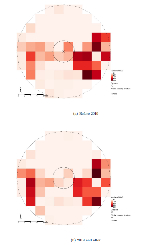
The map presented in figure 4 shows the change in monthly average WVCs per square mile after the WS installation within the seven-mile radius from the WS center. The blue shades correspond to a decrease in WVCs after the WS installation, while the red shades correspond to an increase in WVCs after the installation. White space corresponds to no change in the number of WVCs in the post-intervention period compared to the pre- intervention period. As expected, the majority of the square-mile grids are in blue shades with the WS. Interestingly, there are several red-shaded grids in the potential spillover region on the right end of the WS. However, the map must be interpreted with care as we cannot simply assume there is a reduction in the WS without conducting formal analysis because the changes presented here have not been controlled for any common variants to the treated and control segments in the pre- or post-intervention periods.11For example, the figure does not control for how wildlife cross the road differently during COVID-19, when there was a reduction in traffic volume. Studies have shown that more animals are likely to cross the road if the time interval between cars is longer (Alexander et al., 2005; Riginos et al., 2018). In the control segments where there are no fencing nor overpass, more animals are expected to cross the road when there is less traffic volume. In the formal analysis, this confounding factor can be addressed with the year fixed effect.
Figure 2. Whisker Plot: Average Monthly WVCs
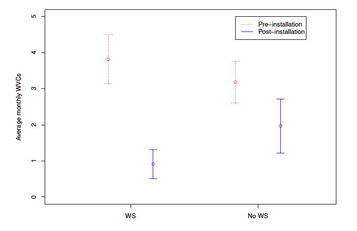
Note: The figure presents the average monthly WVC in the segments that are 0--3.5 miles from the WS centerpoint and 3.5--7 miles from the WS centerpoint before and after the WS is installed. WS  are segments that are 0 to 3.5 miles from the overpass, and No WS
  are segments that are 3.5 to 7 miles from the overpass. Before
  is the all the months from 2010 to 2018, and After
  is all the months on or after 2019. Values of the lower and upper bounds are at the 90 percent confidence interval.
Appendix table A2 reports the frequency distribution of the count of monthly WVCs in each milepost from January 2010 to November 2021, excluding the construction period from April 2018 to December 2018 (Utah Department of Transportation, 2017). I exclude the construction period to avoid any plausible factors that could potentially confound the treatment effect. For example, there are construction zones with reduced traffic speeds during the construction of the WS. Moreover, the increased construction noise and human traffic are likely to deter wildlife from approaching the area, resulting in reductions in WVCs in the control before the WS intervention.
Figure 3. Density Plot: Spatial Distribution of the WVCs in the Pre– and Post–Installation
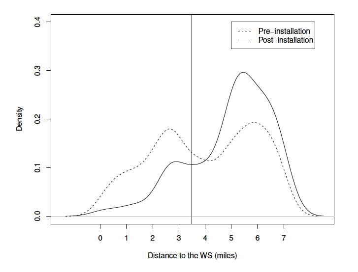
Note: In the figure, 0–3.5 miles are the segments that are within the WS, while 3.5–7 miles are the immediate proceeding segments of the WS. The vertical line marks the end of the WS segments. The kernel density estimate is used to approximate the underlying distribution.
Figure 4. Area of Interest Map: Change in Monthly WVCs
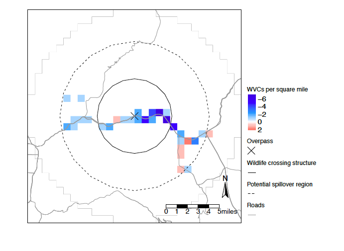
Note: Change in monthly average WVCs per square mile is computed with the seven-mile radius from the WS. The WS is 3.5 miles at both sides, and the potential spillover region is the immediate proceeding 3.5 miles at both sides of the WS.
Empirical Strategy
Because the roadkill data in the count distribution are overdispersed, ordinary least squares (OLS) estimation is likely to result in biased estimation.12In OLS estimation, the error term is assumed to have a population mean of zero, namely normally distributed. However, count distribution is overly dispersed because the count data have many zeros in observation. Thus, I employ negative binomial models to accommodate such a common empirical analysis that uses count data (Cameron and Trivedi, 2005, 2013). The negative binomial distribution is given by
(1) 
where  is a deterministic function of the regressors (
 ) and
) and  is the dispersion parameter. Thus, the distribution has the following properties such that
(2) ![\begin{equation*} \begin{aligned} E[y|\mu,\theta] &= \mu,\\ V[y|\mu, \theta] &= \mu(1+\theta\mu). \end{aligned} \end{equation*}](https://www.thecgo.org/wp-content/ql-cache/quicklatex.com-41c7bf0c09e3261b86834b5c400d346c_l3.svg "Rendered by QuickLaTeX.com")
With such properties, the standard assumption of exponential mean parameterization applies:
(3) 
where  represents the vector of estimated coefficients in the empirical model (Cameron and Trivedi, 2005, 2013).
To quantitatively evaluate the effectiveness of wildlife crossings, I use a DD estimator to control for changes in WVCs independent of the WS installation. COVID-19, for example, impacts traffic volume negatively, which may result in lower WVCs (Liu and Stern, 2021). Alternatively, any policy changes could also result in a decrease or increase in the number of carcasses on the side of the road.13Some states allow salvaging roadkill or have amended their laws to allow roadkill salvage (Botkin, 2019). The preferred specification uses road segments that are in close proximity to the WS due to the similarities in landscape and habitats. Robustness checks with expanded control data along I-80 and the entire state of Utah are presented in the Appendix tables A3 and A4, respectively.
To empirically examine the effect of WS, I fit the panel data to the following equation:
(4) 
where  is the number of monthly roadkill on each milepost in road
  and time
  ,
,  is a dummy variable indicating whether the observation is one of the seven mileposts on I-80 that received the WS treatment effect, and
  is another dummy variable indicating whether the observation is on or after January 2019. The constant terms
  ,
,  ,
,  , and
, and  represent the unknown parameters to be estimated, and
  , which combines fixed effects
  ,
,  ,
,  , and
, and  and the stochastic error term
  . The term represents the full set of route-by-milepost fixed effects, which absorbs all routes by milepost-specific, time-invariant unobserved factors such as topography, landscape, surrounding habitats, and road characteristics that may be correlated with roadkill in each segment. The term is the set of monthly indicators, where the subscript $m$ refers months such that it nonparametrically absorbs all time-varying unmeasured factors such as seasonal change in traffic volume, road conditions, and migration patterns that are common to the specific month(s) of every year. is another set of yearly indicators, where the subscript
  represents each year and absorbs yearly changes in herd unit size, traffic volume, policy changes, outbreak of COVID-19, etc. that are common to the specific year(s). The term represents different regions of the Utah Department of Transportation (UDOT) and the Utah Division of Wildlife Resources. These are the two agencies, each with four and five different subdivisions, respectively, that are responsible for collecting and counting carcasses on the road in the designated regions across Utah. absorbs time-invariant factors common to the specific regions of the two departments.
To isolate and identify the potential spillover effects (that could be positive or negative), I conduct a donut analysis on both ends of the WS and both ends of the overpass with changing donut size sample specifications. The original control samples in the main analysis are the 3.5- to 7-mile observations from the end of the WS, while the donut control samples are 4.5- to 7-mile observations and 5.5- to 7-mile observations from the end of the WS. The rationale behind doing this is that the area of the spillover segments is unknown, and thus excluding segments at the end of the structure helps guard against the possibility of confounding effects from the potential spillover-impacted segments near the WS. The results and discussion are presented in Section 5.2.
Finally, for the DD estimator to be valid, the parallel trend assumption must be met, which means that in the absence of treatment, the difference between the treated and control segments should be relatively constant over time. Figure 5 allows me to visually confirm whether or not this assumption is met. The vertical line indicates when the WS was installed and in use. During the pre-installation period (left of the vertical line), both the treated and control segments exhibit a similar trend, with the treated segments consistently higher than the control segments. During the post-installation period, the control segments have constantly higher monthly WVCs than the treated segments. These results provide evidence to the parallel trend assumption is being satisfies in this case. To the right of the vertical line, the treated group experiences a sharp decline, approximately 0.4 in quarterly average WVCs per mile.
Figure 5. Parallel Trend: Quarterly Average WVCs
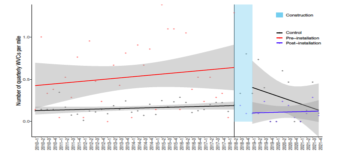
Note: The figure shows the first-order polynomial approximation of the control group and the treated group in the pre– and post–installation in the seven-mile radius from the WS on I-80.
Results
Effect of the WS on WVCs
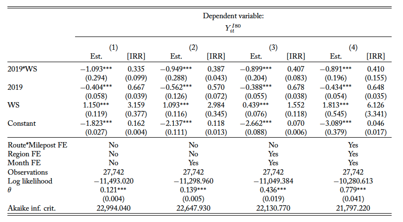
Table 4 presents the results from estimating equation 4 with the preferred I-80 sample within seven miles of the WS center. The results with the I-80 sample and the statewide sample can be found in Appendix tables A3 and A4, respectively. The results in column 1 of table 4 and Appendix tables A3 and A4 correspond to the baseline models with the corresponding sample and no corrections for any fixed effect. Column 2 reports results from adding month fixed effects, and the specification in column 3 adds another full set of region fixed effects. Column 4 presents the preferred specification, which includes the full set of routes by milepost fixed effects. Overall, the preferred specification—whether with the full sample, a subset on I-80, or a subset on I-80 and in close proximity with the WS structure—yields qualitatively similar estimates of the effect of receiving the WS intervention (I-80 sample: 59.0 percent; statewide sample: 69.5 percent), and from the Akaike information criterion, adding the fixed effects improves the overall model precision. I find empirical evidence that installing the WS with fencing on both sides of the structure results in an immediate and quantifiable decrease in WVCs. Column 4 in table 4 shows an approximately 66.1 percent reduction (incident rate ratios14IRRs for the negative binomial estimation are interpreted as treated outcome = IRR × counterfactual outcome. (IRR)) at the 1 percent level of significance, ceteris paribus, due to the implementation of the WS. Across various fixed effect models, the estimates are very similar in magnitude (column 1, 65.6 percent; column 2, 64.2 percent; column 3, 62.5 percent).
Table 4. I-80 and within 7-Mile Radius Sample: Effect of WS on WVCs
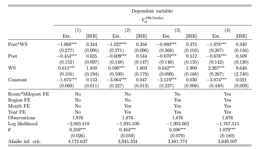
Note: The dependent variable is the count of monthly roadkill per month for each milepost on each road. Columns 1–4 report results for the analyses with a subset of the I-80 sample within seven miles of the WS center. All regressions follow a negative binomial distribution. Column 1 reports results from the baseline regressions with no fixed effects, and column 2 reports results from adding month fixed effects. Column 3 reports results from adding month and region fixed effects, and column 4 reports results from adding full set of fixed effects including month, region, and route by milepost fixed effects. ∗p<0.1; ∗∗p<0.05; ∗∗∗p<0.01
Falsification Tests
The following falsification tests (figure 6 (a)) are performed on observations before 2019 as if they were the treatment years and performed on the rest of the observations before the construction (April 2018) as controls. The purpose of this exercise is to detect if there is any other measurable effect of treated segments experiencing a reduction in WVCs before the intervention. As shown in figure 6, most of the point estimates are above zero and statistically insignificant. Interestingly, the 2018 point estimate is below zero and statistically significant. However, the WS construction was an on-going project for seven months in 2018, and it is very likely that the reduction is due to WS construction deterring wildlife from approaching the area. This further justifies omitting observations that fall within the construction periods (April 2018 to December 2018). In figure 6 (b), the pre-intervention observations are grouped into three-year intervals, with the last estimation being the same estimation as in the main analysis in table 4, column d. This figure allows me to directly compare the various falsification samples of some fabricated intervention periods (2010–2012, 2013–2015, 2016–2018) to the actual intervention period (2019–2021).
Potential Spillover Effect at WS Fence Ends
There have been contradictory findings regarding the negative spillover effects of WVCs at fence ends (Clevenger et al., 2001; Huijser et al., 2016), and no study has evaluated this issue with quantitative analysis. Therefore, this section examines and identifies the control segments that could potentially experience spillover with two strategies, both of which use the same estimation method as in equation 4.
The first strategy assigns the current control segments as treated and the immediate proceeding segments are assigned as controls. The analysis is performed with three specifications to verify potential spillover effects on the east side of the WS, as presented in figure 4. The first specification consists of the entire control segments as treated, the second consists of the east side of the control segments as treated, and the third consists of the west side of the control segments as treated. The results are presented in table 5. The second strategy, a donut specification, excludes control observations that are within one and two miles of the treated segments, respectively. Similar to the first strategy, there are also three specifications with the donut analysis. Each of the point estimations are illustrated in figure 7.
Figure 6. Falsification Tests: By Year and 3–Year Intervals
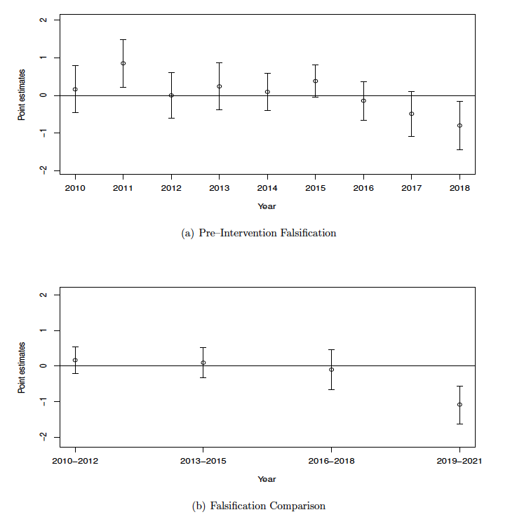
Note: Panel (a) presents each of the pre–intervention periods treated as if those are the periods receiving intervention, while panel (b) presents the comparable estimations by grouping the pre–intervention periods with the same three–year interval. Point estimates are the coefficient of the variable of interest as in equation 4.
Spillover Regression
Table 5 shows that using the sample from both the two-mile ends of the WS and the immediate two-mile segments yields a positive estimate ( ), although it is not statistically significant. However, as indicated in figure 4, the spillover effect seems to be present on the east side of the WS. To explore this further, I separate the sample into the west and east sides. The west side estimation (
 ) is as expected and consistent with that in column 1, but the east side sample reveals a positive estimate (
 ) of a 205 percent increase in WVCs (which translates into 13.18 more accidents per year) after the WS implementation on the east side at the 10 percent statistical significance level. This finding suggests that the reduction effect of WS could be overestimated if the spillover effect found on the east end of the WS is not accounted for.
Donut Analysis
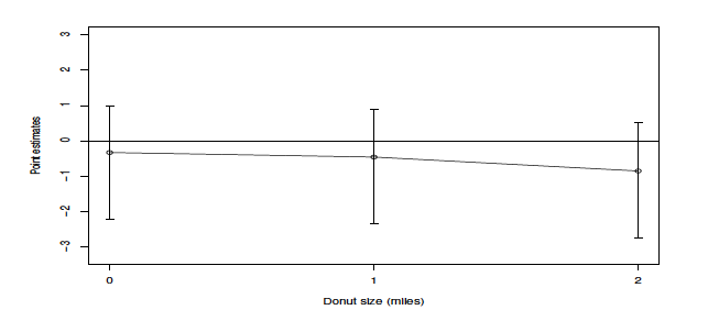
Figure 7. Spillover Effect at Structure Ends: Donut Specifications
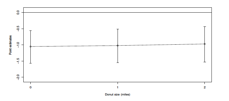
Note: The donut size indicates the size of the donut area such that control observations that fall into the area are excluded from the analysis. Point estimates are the coefficient of the variable of interest as in equation 4.
A donut size of 0 (figure 7) is the same estimate as in the preferred specification in table 4, column 4. To interpret the donut analysis result, I compare estimates of different donut sizes. If the variation is small, this suggests there is no spillover effect, and if there is a reduction in the effect, it suggests there is a positive spillover of WVCs to the control segments due to the WS and vice versa. As presented in figure 7, the variation of the coefficient estimates is very small (less than 0.05 units in the point estimate or 1.844 percent in WVC reduction compared to the estimation in the main analysis), it does not suggest evidence of spillover (neither positive nor negative). To investigate this further, two more specifications were performed following the approach in Section 5.2.1, one on the east side and one on the west side. The results are shown in figure 8.
Table 5. Spillover Sample: Spillover Effect of WS
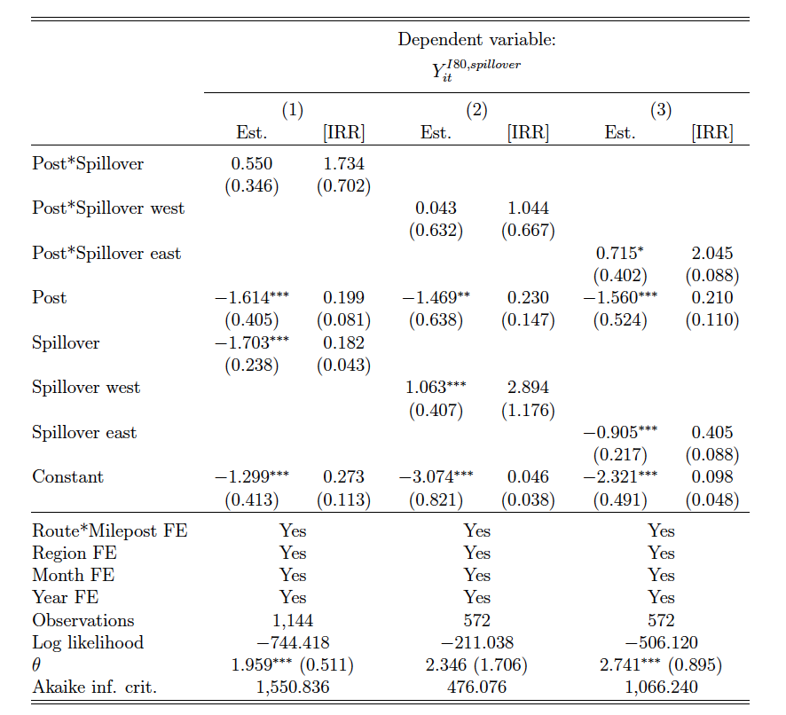
Note: The dependent variable is the count of monthly roadkill per month for each milepost on each road. Column 1 reports results from the analysis with the I-80 sample and the last two miles of the WS on both sides and the immediate proceeding two miles of the WS on both sides. Column 2 reports results from the analysis with the I-80 sample and the last two miles of the WS on the west sides and the immediate proceeding two miles of the WS on the west sides. Column 3 reports results the analysis with the I-80 sample and the last two miles of the WS on the east sides and the immediate proceeding two miles of the WS on the east sides. All regressions follow a negative binomial distribution and include a full set of fixed effects (i.e., month, region, and route by milepost fixed effects). ∗p<0.1; ∗∗p<0.05; ∗∗∗p<0.01
Notably, the figure shows that a higher reduction effect is observed on the west side compared to the east side of the WS and becomes insignificant starting at the donut size of one mile in the east side sample. The estimates from the east side sample suggest a spillover effect, indicating that the WS is generating more WVCs at its ends and is potentially creating another hotspot. This finding emphasizes the importance of considering spillover effects when evaluating the impact of human interventions that mitigate WVCs like the WS. The reason why the spillover effect only presents on one side of the WS is unclear, but it may be due to differences in the surrounding landscape and the road design. Future research should investigate these factors to better understand their role in shaping spillover effects. An additional set of donut specifications at the overpass ends is presented in Appendix D.
Event Study Analysis
This event study analysis exploits the variation in the reduction in WVCs over time to identify the effect of the WS in reducing WVCs. Applying the model below, I assume that the number of roadkill,  , in milepost at time
  , where is a given year and month
  (
( ), is characterized by
(5) 
where is defined similarly as equation 4 and  is the measure of the yearly treatment effect owing to the WS installation.
  is also defined similarly as equation 4 with the only difference being that it does not contain the year fixed effect as in
  . Since the estimates are binned every year, the year when the construction occurred (year 2018) was omitted from the sample and the year before the intervention (year 2017) was omitted from the regression.
Figure 8. Donut Analysis: West and East Side Sample
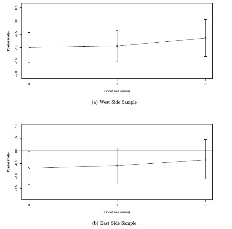
Note: The donut size indicates the size of the donut area such that control observations that fall into the area are excluded from the analysis. Point estimates are the coefficient of the variable of interest as in equation 4. Panel (a) presents the donut analysis using the west side sample, while panel (b) presents the donut analysis using the west side sample.
Figure 9. Event Study: Yearly Treatment Effect
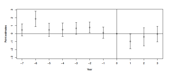
Note: This figure plots the event study coefficient estimates from the model outlined in equation 5. Estimates are based on negative binomial models using monthly-by-milepost data from the Utah Department of Transportation. The outcome variable is the number of roadkill for a given milepost in a given month. The bars show the 90 percent confidence interval. The coefficients for the year before the WS installation are omitted from the regression, and the year when the construction took place is also omitted. The omitted period from the regression is indicated as year zero and the vertical line. Point estimates are the coefficient of the variable of interest as in equation 5.
Figure 9 plots the yearly coefficient estimates and the 90 percent confidence interval of the treatment effect indicator from equation 5. Year zero represents the period before the intervention. The estimate at year one corresponds to the change in WVCs one year after the WS installation, the estimate at year two after the WS installation, and so on. The figure shows mostly no significant effects on the reduction in WVCs in the year leading up to the WS installation, which reinforces the causal direction of the estimation. In the immediate proceeding year after the WS installation, I observe a coefficient estimate of approximately –1.08, which can be translated to a 66.3 percent reduction in WVCs in the area owing to the WS installation. While the second and third year after the intervention are not statistically significant, this is very likely to due to a change in traffic volume due to COVID, which in turn changed the behavior of wildlife crossing the road. Existing studies have shown that wildlife make different decisions crossing the road when there are varying time intervals between cars (Alexander et al., 2005; Riginos et al., 2018). The full event study regression result is presented in Appendix table A6.
When traffic volume returns to pre-COVID period levels, I assume that wildlife cross- ing behaviors return to the pre-COVID period. It is reasonable to suspect that the estimate of the 66 percent reduction in WVCs in the main analysis, which is the average treatment effect including the COVID years, could underestimate the real impact of the WS. Therefore, I rerun the main analysis with the pre-COVID sample and present the results in Appendix table A5.
Robustness Checks
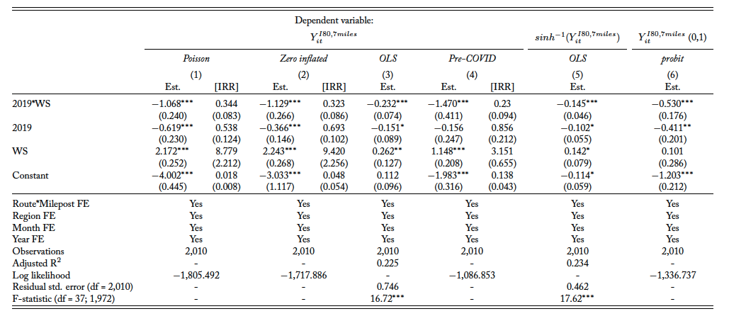
Several sets of robustness checks were performed to further verify the validity of the main results. Column 1 of Appendix table A5 presents the same specification estimation with a Poisson distribution instead of the negative binomial distribution. Expectantly, it gives a similar estimation as in the binomial distribution. As Greene (1994) suggests that excess zeros can masquerade as overdispersion, the next column presents the zero-inflated negative binomial distribution result. This is an approach using the two-stage Heckman approach, with the first stage predicting whether the zeros in the outcome variables are sampling zeros or structural zeros. The outcome variables’ lag and two lags are used as the regressors for the dependent outcome variable. Accounting for a potential excess zero problem, the estimation arrives at a 67.7 percent reduction compared to 66.0 percent in the main analysis, which is negligible.
Columns 3 and 4 present the estimation in OLS, with column 3 showing the count outcome under no transformation and column 4 showing the count outcome under inverse hyperbola sine transformation. Similar to log transformation, inverse hyperbola sine helps to transform the skewed data to a normal distribution while also handling zeros without crudely transforming the data (Gibson et al., 2017). In both instances, I observe negative estimations.15I do not translate the estimation for direct comparison because OLS estimates are biased in count distribution data, which is undesirable. The main purpose here is to show the consistent signs.
For further validation, I perform a probit regression (column 5) with outcome variables classified as binary variables, where they equal one if there is any roadkill in a specific milepost at a specific month and zero otherwise. I find a 51.6 percent reduction on any monthly WVC in a specific milepost. Scaling up to the average number of WVCs if a milepost of a given month has any WVC in the treated segments, it translates to a 69.9 percent reduction in WVCs. Last but not least, I further limit the sample to the pre-COVID 19 period. As presented in column 6, the WS is effective in reducing WVCs by 76.9 percent. The higher estimate here suggests that in the absence of COVID 19, it is expected to see a higher reduction effect, in which this higher estimate will be used as the high estimate in calculating the benefit of the WS.
Cost-Benefit Analysis and Policy Implications
Public infrastructure often has a high cost that needs to be justified with the future benefit it will provide. With WSs typically costing millions of dollars, this section focuses on the lifetime value of the studied WS. The following benefit-cost analysis (BCA) is done by assuming the WS has a service life of 75 years16After communicating with the UDOT and the engineering team that designed and built this over-pass, I learned this overpass has an expected service life of 75 years and only needs to be maintained every 20–30 years. and is discounted at 3 percent, which is commonly assumed in the social discounting of environmental investments (Office of Management and Budget, 2017).
To estimate the benefit generated from avoided collisions, this exercise assumes a constant rate of future WVCs given that the percentage of WVCs to all types of vehicle collisions in Utah stays relatively constant (table A8).17The percentages of statewide WVCs compared to all types of vehicle collisions are around 2.6 percent in the past 11 years. The percentages of I-80 WVCs compared to all types of vehicle collisions are around 5 percent in the pre-intervention periods (2010–2017). The percentages of preferred sample (I-80 and within a seven-mile radius) WVCs compared to all types of vehicle collisions are around 12.5 percent in the pre-intervention periods (2010–2017). While this BCA aims to provide the most accurate estimate possible, there are many unobserved factors that could affect the future expected number of WVCs in the studied area or data limitations on making different assumptions on the expected future WVCs. For example, technology advancement might be able to reduce the likelihood of hitting wildlife in the future, but there is not enough information on vehicle safety measure effectiveness at reducing WVCs. Second, while commuters could change driving patterns or use alternate routes, using the interstate is the most direct route and any detours could lead to an extra 90 minutes of driving time in the studied region (Associated Press, 2018). Therefore, it is unlikely that this factor would contribute to a change in the expected WVCs in the near term. Third, although it is reasonable to believe that wildlife density may change over time, this BCA uses an eight-year average WVC in the studied area in the pre-intervention periods, which should account for some of the density changes over time. The distribution of WVC types is based on the eight-year pre-intervention history, and is then multiplied by the corresponding collision cost estimate presented in table 1. The resulting average collision cost is then multiplied by the eight-year pre-intervention average number of WVC in the WS area, and discounted by the reduction rates obtained from the regression results (i.e., 66.1 percent reduction rate in the lower estimate and the 76.9 percent reduction rate in the higher estimate). The sum of the future benefit is discounted back to the present value using a social discount rate of 3 percent.
According to UDOT open records, this wildlife overpass and fencing cost $5 million to construct and is part of the $22 million I-80 Westbound Truck Lane project in the Parleys Summit to Jeremy Ranch in Summit County that is funded with federal dollars (Utah Department of Transportation, 2017). From the date of completion (December 2018) of the WS to present, there is one maintenance record in November 2021 of $136,167 that is funded with state dollars (Utah Department of Transportation, 2021). As the structure does not carry any traffic weight, maintenance is only required every 20–30 years. This exercise uses the most stringent level of maintenance, which is every 20 years, and costs $136,167 each time. With evidence of a positive WVC spillover at the WS fence ends, this BCA includes the cost of spillovers present as a result of the WS. Finally, the remaining cost of WVCs that are not prevented by the WS and the cost of WVCs when there are no WSs are also included in the total cost under the corresponding categories. The sum of the future costs is discounted back to the present value using a social discount rate of 3 percent.
Notably, WS provides a substantial benefit from saved collisions regardless of whether the high estimate or low estimate is assumed. The estimated benefit is between 2.48 and 2.13 times the cost of construction and maintenance (Appendix table A7). However, this estimate may be overstated due to the presence of a positive spillover effect and because the WS does not eliminate all WVCs. As a result, the net social benefit is negative under any scenario. Nevertheless, compared to not having the WS at all, there are significant improvements in having one as suggested in the net social improvement in table 6.
It is worth noting that the cost-benefit analysis here does not account for the positive externality that the WS offers in connecting habitats and promoting biodiversity.
Table 6. Benefit-Cost Analysis: Comparison of Present Values with and without WS Infrastructure
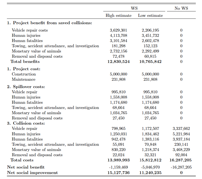
Note: The average service life of wildlife overpass in the US (75 years) is assumed. Collision costs are converted into 2022 USD. The proportion of animals involved in the WS are used to derive collision costs reflected in benefit. All estimates are discounted at 3 percent, which is commonly assumed in social discounting of environmental investments (Office of Management and Budget, 2017).
Adopting the Huijser et al. (2008) estimate, any deer, elk, and moose are valued equally at $2,000–$3,000, which does not necessarily reflect the true value in the region. According to Siu et al. (2023), an average elk has a stock-dependent shadow value estimated to be approximately $6,000 on average and can range from $2,300 to $11,000 depending on the herd unit or location. Meanwhile, an average mule deer has a stock-dependent shadow value estimated to be approximately $1,750 on average and can range from as low as $300 to as high as $2,700 depending on the herd unit or location.18The shadow price is hunting explicit and is the revealed willingness to pay by the hunters. It is stock dependent because hunter willingness to pay depends on the stock size and herd unit. Further, the amount of licenses being issued to hunters is also stock dependent. The shadow price has been accounted for in the cost of per head management and the cost of a hunting trip. The reduction in WVCs promotes not only the benefit from prevented collisions, but also the ecological benefit, which is not counted into the benefit. Therefore, the BCA presented here provides only a lower limit.
As the interstate has high traffic volume and drivers from both in and out of state, exploring the distribution of in- and out-of-state drivers involved in WVCs can be insightful for policymakers in attributing the cost of an expensive infrastructure. According to the vehicle characteristics of Utah WVC crash data for I-80 on the seven treated mileposts, 77.4 percent are in-state vehicles versus 22.6 percent of out-of-state vehicles. In other words, a majority of the benefit of the WS goes to in-state drivers. With the WS being funded entirely by federal dollars, the state of Utah has an opportunity to improve road safety and save money by investing in wildlife infrastructure itself instead of solely relying on federal funding. The state has been responsible for the maintenance cost of the WS, which is 1/22 of the total cost of the WS in present value; this is far less than the benefit provided to in-state drivers. In the last two budget cycles, 2021–2022, the state of Utah invested more than $2.1 billion in transportation (Utah State Legislature, 2022). Even if the state took on more of the initial construction costs, the cost-benefit ratio would still pay off thanks to the reduction in WVCs and their associated costs.
Conclusion
Enhancing safety for drivers and wildlife can be improved by increasing the understanding of social benefits that flows from new and expensive wildlife crossing infrastructure. This paper addresses overdispersed roadkill data with a DD model with a negative binomial distribution. Using the novel daily per carcass data, I find that installing a WS reduces WVCs by 66 to 77 percent, and the effect is immediate. This finding diverges from previous findings that it generally takes three years for wildlife to adapt to a new WS (Cramer, 2013). Although the implementation of WS has been shown to significantly reduce the number of WVCs, this study has identified a positive spillover effect of WVCs. This suggests that WS potentially push WVCs further away from their location, resulting in a shift in the location of roadkill hotspots rather than a complete elimination of the problem. While the net effect still shows a reduction in WVCs, this finding highlights the importance of carefully considering the placement and design of WSs and their potential impact on wildlife behavior. In order to fully realize the benefits of WSs, it is crucial to design them in a way that minimizes the negative spillover effects and maximizes their effectiveness in reducing WVCs. Properly placed and designed WSs can help to enhance safety for both drivers and wildlife, and reduce the financial burden of WVCs.
On the other hand, the sources of biased estimates from previous studies are clearly illustrated and discussed in Section 3 and in table 2. Whether formal analysis is not possible, or a quick evaluation is desired, this paper argues that future studies and reports quantifying the effect of WS must account for the differences in time-varying factors between the pre- and post-intervention periods as well as differences between the treated and control areas.
Using in- versus out-of-state characteristics in the studied region, I also estimate that the net social improvement is valued more than 15 million USD and the estimated benefit outweighs the cost by more than double over the service life of the WS. This expensive public infrastructure is mostly funded with federal dollars, but with 77 percent of the benefit generated directly benefiting in-state drivers and 23 percent benefiting out-of-state drivers, it appears that public infrastructure to mitigate WVCs should be funded collaboratively by state and federal stakeholders.
Finally, as insurance companies are often responsible for the high costs resulting from WVCs and associated injuries, it is worth considering whether they can benefit from investing in WSs. These WSs have been shown to be highly effective in reducing the number of WVCs, which can help insurance companies save money by avoiding expensive claims for vehicle damage and bodily injuries. Additionally, WSs can also help to reduce the number of accidents caused by drivers swerving to avoid hitting animals, which can also result in costly claims. Therefore, investing in WSs can be a cost-effective way for insurance companies to minimize their financial risks and promote safety for both drivers and wildlife.
Appendix
A. Tables
Table A1. Top 5 Big Game Animals Involved in WVCs in Utah, 2010–2021
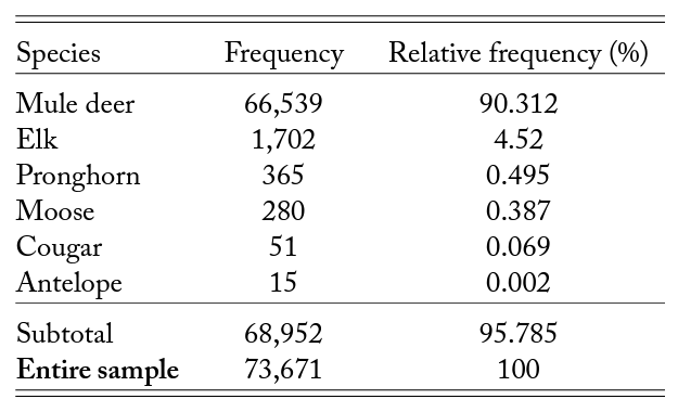
Note: WVC data from 2010 to 2021 are obtained from the Utah Department of Transportation. The frequency count of big game animals involved in WVCs in Utah is computed for the years 2010–2021.
Table A2. Roadkill: Actual Frequency Distribution, 2010–2021
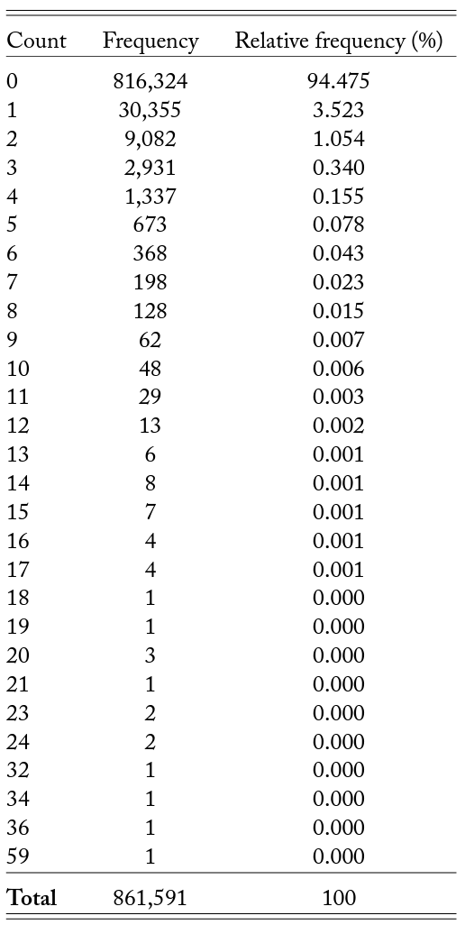
Note: WVC data from 2010 to 2021 are obtained from the Utah Department of Transportation. The frequency of monthly WVCs per mile is computed for the study period.
Table A3. I-80 Sample: Effect of WS on WVCs
Note: The dependent variable is the count of monthly roadkill per month for each mile on each road. Columns 1–4 present results for the analyses with a subset of the I-80 sample. All regressions follow a negative binomial distribution. Column 1 reports results with no fixed effects, and column 2 reports results from adding month fixed effects. Column 3 presents results from adding month and region fixed effects, and column 4 presents results from adding the full set of fixed effects including month, region, and route by milepost fixed effects. ∗p<0.1; ∗∗p<0.05; ∗∗∗p<0.01
Table A4. Statewide Sample: Effect of Wildlife Crossings on WVCs
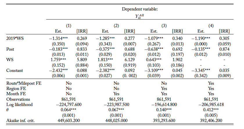
Note: The dependent variable is the count of monthly roadkill per month for each mile on each road. Columns 1–4 are the analyses with the full sample. All regressions follow a negative binomial distribution. Column 1 reports results with no fixed effects, and column 2 reports results from adding month fixed effects. Column 3 reports results from adding month and region fixed effects, and column 4 reports results from adding the full set of fixed effects including month, region, and route by milepost fixed effects. The coefficient estimate for the WS in column 4 is very large and thus omitted in reporting. ∗p<0.1; ∗∗p<0.05; ∗∗∗p<0.01
Table A5. Robustness Checks
Note: The dependent variable is the count of monthly roadkill per month for the seven-mile radius from the WS on I-80 without transformation in columns 1–3, with a hyperbola sine transformation in column 4, and with a binary indication in column 5. ∗p<0.1; ∗∗p<0.05; ∗∗∗p<0.01
Table A6. Event Study: Regression
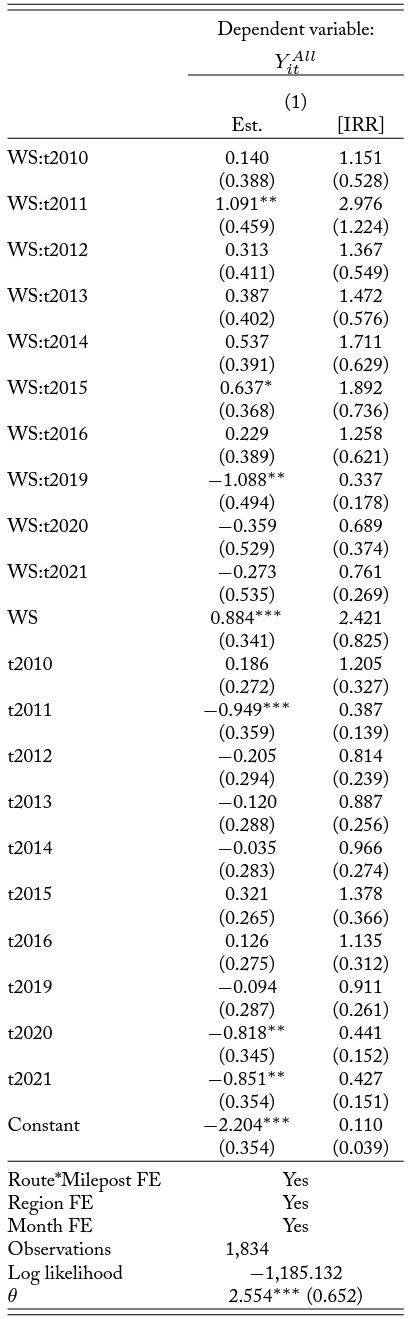
Table A7. Benefit-Cost Analysis: Benefit of Reduced WVCs and Cost of the WS Infrastructure over Its Service Life
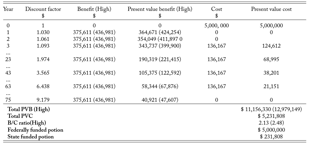
Note: The average service life of bridges in the US is assumed. Collision costs were converted in 2022 USD. The proportion of animals involved in the WS are used to derive collision cost reflected in benefit.
Table A8. Vehicle Crash and Wildlife Vehicle Crash Report in Utah, 2010–2021
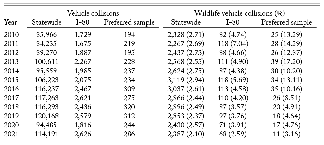
Note: Crash report data from 2010 to 2021 are obtained from the Utah Department of Public Safety. The count of all type of collisions are presented in columns 1–3, and the count of wildlife vehicle collisions are presented in columns 4–5. Percentages presented in parentheses are based on vehicle collisions in the same category (i.e., statewide, I-80, and WS).
B. Figures
Figure B1. Density Plot of WVCs of the Entire Sample to the Overpass, 2010–2021
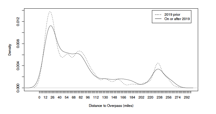
Figure B2. Density Map of WVCs at WS
C. Heterogeneity Effects on Different Big Game Species
The WS was built to prevent and reduce WVCs in the Parleys Canyon, which is the major hotspot of WVCs in Utah. However, how different species of wildlife use different types of wildlife crossings can lead to varying levels of effectiveness. The WS studied in this paper is a wide overpass accompanied with fencing, which is one of the most versatile types of crossing structures for a wide range of wildlife (Clevenger and Huijser, 2011). To evaluate the effectiveness of this WS in Parleys Canyon, Utah for the top three big game animals involved in WVCs in the area, the following analysis (see Appendix table C1) focuses on each of them, i.e., deer, elk, and moose, respectively.
With mule deer accounting for over 86 percent of all crashes in the area, the 66.4 percent reduction in deer vehicle collisions at the 1 percent significance level is encouraging. Although the reduction in elk or moose vehicle collisions is not statistically significant, the estimates show the expected negative signs.
Table C1. Heterogeneity Effect: Top 3 Big Game WVCs
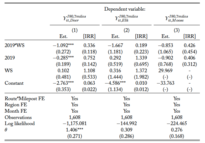
Note: The dependent variable is the count of monthly roadkill of the corresponding big game animals per month for each mile on I-80 within seven miles from the WS centerpoint. Some estimates and standard errors for moose in column 3 are omitted because they are uninterpretable. ∗p<0.1; ∗∗p<0.05; ∗∗∗p<0.01
D. Spillover Effect at Overpass End
I perform an additional set of donut specification by omitting the preceding one and two- mile segments from the overpass (figure D1). Despite the larger reduction effect when removing observations that are closer to the overpass, which suggests that the reduction is less effective on WVCs that are further from the overpass, the estimation is statistically insignificant.19Any change in the coefficient estimate compared to the point estimate at the zero donut size (full sample) may be due to either changes in control observations because of the intervention or to differences in the controls that are not being captured by the model. When the coefficient estimate magnitude is larger (more negative) when omitting control observations closer to the treatment group, it means there are more WVCs at the remaining control observations than the ones that are omitted and vice versa.
Figure D1. Spillover Effect at Overpass End: Donut Specifications
Note: The donut size indicates the size of the donut area such that control observations that fall into the area are excluded from the analysis. Point estimates are the coefficient of the variable of interest as in equation 4.
References
Alexander, S., Waters, N., and Paquet, P. (2005). Traffic volume and highway permeability for a mammalian community in the Canadian Rocky Mountains. The Canadian Geographer/Le G´eographe Canadien, 49:321–331.
Allen, R. E. and McCullough, D. R. (1976). Deer-car accidents in Southern Michigan. The Journal of Wildlife Management, 40(2):317–325.
Associated Press (2018). Interstate 80 to Close for Wildlife Overpass Project.
Benten, A., Hothorn, T., Vor, T., and Ammer, C. (2018). Wildlife warning reflectors do not mitigate wildlife—Vehicle collisions on roads. Accident Analysis & Prevention, 120:64–73.
Bissonette, J., Kassar, C., and Cook, L. (2008). Assessment of costs associated with deer–vehicle collisions: Human death and injury, vehicle damage, and deer loss. Human Wildlife Conflicts, 2:17–27.
Botkin, B. (2019). Law allowing salvage of roadkill proves popular. New York Times.
Bruinderink, G. W. T. A. G. and Hazebroek, E. (1996). Ungulate traffic collisions in Europe. Conservation Biology, 10(4):1059–1067.
Caldwell, M. R. and Klip, J. M. K. (2021). Mule deer migrations and highway underpass usage in California, USA. The Journal of Wildlife Management.
Cameron, A. C. and Trivedi, P. K. (2005). Microeconometrics: Methods and Applications. Cambridge University Press.
Cameron, A. C. and Trivedi, P. K. (2013). Regression Analysis of Count Data, volume no. 53. Cambridge University Press.
Clevenger, A. P., Chruszcz, B., and Gunson, K. E. (2001). Highway mitigation fencing reduces wildlife-vehicle collisions. Wildlife Society Bulletin, pages 646–653.
Clevenger, A. P. and Huijser, M. P. (2011). Wildlife Crossing Structure Handbook: Design and Evaluation in North America. Federal Highway Administration.
Conover, M., Pitt, W., Kessler, K., DuBow, T., and Sanborn, W. (1995). Review of human injuries, illnesses, and economic losses caused by wildlife in the United States. Wildlife Society Bulletin, 23:407–414.
Cramer, P. (2013). Design recommendations from five years of wildlife crossing research across Utah. Technical report, Proceedings of the 2013 International Conference on Ecology and Transportation.
Cramer, P., Kintsch, J., Gagnon, J., Dodd, N., Brennan, T., Loftus-Otway, L., Andrews, K., Basting, P., LoranFrazier, and Sielecki, L. (2022). The Strategic Integration of Wildlife Mitigation into Transportation Procedures: A Manual for Agencies and Partners. Nevada Department of Transportation.
Donalson, B. M. and Elliott, K. E. M. (2020). Enhancing existing isolated underpasses with fencing reduces wildlife crashes and connects habitat. Human–Wildlife Interactions, 15(1).
Federal Highway Administration (2021). Bipartisan infrastructure law. Technical report, U.S. Department of Transportation.
Gibson, J., Datt, G., Murgai, R., and Ravallion, M. (2017). For India’s rural poor, growing towns matter more than growing cities. World Development, 98(C):413–429.
Greene, W. (1994). Accounting for excess zeros and sample selection in Poisson and negative binomial regression models. NYU working paper No. EC-94-10.
Helean, J. (2022). UDOT reveals how many animals used I-80 Parley’s Canyon crossing in 2021. https://www.fox13now.com/news/local-news/udot-reveals-how-many-animals-used-i-80-crossing-in-parleys-canyon-in-2021.
Huijser, M. P., Duffield, J. W., Clevenger, A. P., Ament, R. J., and McGowen, P. T. (2009). Cost–benefit analyses of mitigation measures aimed at reducing collisions with large ungulates in the United States and Canada: A decision support tool. Ecology and Society, 14(2).
Huijser, M. P., Fairbank, E. R., Camel-Means, W., Graham, J., Watson, V., Basting, P., and Becker, D. (2016). Effectiveness of short sections of wildlife fencing and crossing structures along highways in reducing wildlife–vehicle collisions and providing safe crossing opportunities for large mammals. Biological Conservation, 197:61–68.
Huijser, M. P., McGowan, P., Clevenger, A. P., Ament, R., Berger, L., et al. (2008). Wildlife-Vehicle Collision Reduction Study: Best Practices Manual: Report to Congress. US Department of Transportation Federal Highway Administration.
Kammerle, J.-L., Brieger, F., Kroschel, M., Hagen, R., Storch, I., and Suchant, R. (2017). Temporal patterns in road crossing behaviour in roe deer (Capreolus capreolus) at sites with wildlife warning reflectors. PLOS One, 12(9):e0184761.
Liu, Z. and Stern, R. (2021). Quantifying the traffic impacts of the COVID-19 shutdown. Journal of Transportation Engineering, Part A: Systems, 147(5):04021014.
McCollister, M. F. and Manen, F. T. V. (2010). Effectiveness of wildlife underpasses and fencing to reduce wildlife-vehicle collisions. Journal of Wildlife Management, 74(8):1722–1731.
Office of Management and Budget (2017). Discounting for public policy: Theory and recent evidence on the merits of updating the discount rate. https://obamawhitehouse.archives.gov/sites/default/files/page/files/201701_cea_discounting_issue_brief.pdf.
Riginos, C., Fairbank, E., Hansen, E., Kolek, J., and Huijser, M. P. (2022). Reduced speed limit is ineffective for mitigating the effects of roads on ungulates. Conservation Science and Practice, page 618.
Riginos, C., Smith, C., Fairbank, E., Hansen, E., and Hallsten, P. (2018). Traffic Thresh- olds in Deer Road-Crossing Behavior. State of Wyoming Department of Transportation.
Siu, W. Y., Bennett, D., Kirkland, B., and Jacob, H. (2023). Natural wealth, externalities and restitution pricing. Working Paper.
State of California (2022). Liberty Canyon wildlife crossing. https://smmc.ca.gov/liberty-canyon-wildlife-corridor/.
Utah Department of Transportation (2017). I-80; Parleys Summit to Jeremy Ranch WB Truck Lane.
Utah Department of Transportation (2021). I-80; Parleys Summit Bridges.
Utah State Legislature (2022). Lanes, trains, and automobiles: a closer look at general fund investments in transportation. Technical report, General Fund Transportation Projects, CY 2021-2022.
Western Transportation Knowledge Network (2021). US state DOT wildlife crossing structures. https://transportation.libguides.com/c.php?g=849313&p=6075360.