


 Policy Commons
1. Introduction
In financial markets, settlement refers to the seller’s obligation to produce a certificate and executed share-transfer form to exchange with the buyer for a corresponding payment.1Settlement cycles have evolved from delivering physical security certificates to delivering electronic share-transfer forms via an electronic settlement system. Clearing a transaction occurs between the trade date and settlement date, which involves any modifications needed to facilitate settlement. The settlement cycle, or period, is the time between the transaction date and the settlement date.2The transaction date marks the date that the buyer and seller agree to trade, whereas the settlement date marks the date the seller delivers the security’s certificate and the buyer transfers the appropriate funds. The Securities and Exchange Commission (SEC) dictates the allowable time within which to settle a transaction in US financial markets. The settlement cycle is widely referred to as T+x, representing the trade date (T) plus the number of business days (x). For over two decades, the SEC has required equity transactions to be settled on a T+3 basis. However, the global credit-and-liquidity crisis of the late 2000s led the SEC and the Depository Trust and Clearing Corporation (DTCC) to rethink the risks and costs associated with a prolonged settlement cycle. On September 5, 2017, the SEC adopted Rule 15c6-1(a), which shortened the standard settlement cycle for nearly all broker-dealer equity transactions from T+3 to T+2.
In this paper, we examine the effects of a shortened standard settlement cycle on firm-level liquidity. Most equity security transactions involve the services of specialized financial intermediaries, such as broker-dealers or central-counterparty members. These intermediaries essentially conduct a two-sided auction, as they stand ready to trade on the buy (long) or sell (short) side of the market (O’Hara and Oldfield 1986). Facilitating such trade requires capital.3https://www.sec.gov/rules/concept/s72499/broy1.htm. When intermediaries buy a security, they can service the trade using their own capital or borrow in the lending market using the security as collateral. However, intermediaries cannot borrow the entire value of the position. The difference between the security’s value and collateral value, also known as margin, must be financed with the intermediaries’ own capital. Similarly, when intermediaries sell a security, they can float the transaction with their own inventory or short sell by borrowing the shares. Short selling, however, requires capital in the form of margin; it does not free up capital. Since intermediaries do not typically carry large long positions in inventory, they must sell short to meet sudden buying demands of market participants. Thus financial intermediaries can face borrowing constraints on both long and short positions.
Brunnermeier and Pedersen (2009) construct a theoretical model that links an asset’s market liquidity to intermediaries’ funding constraints. The authors argue that the ease with which funding can be obtained by traders affects market liquidity. If funding is tight, intermediaries become reluctant to take on positions in high-margin securities, and as a result, market depth declines for those securities. Furthermore, an intermediary’s risk from holding a security is a determinant of the bid-ask spread (Tinic 1972, Tinic and West 1972, Branch and Freed 1977, Hamilton 1978, and Stoll 1978), which measures the size of the transaction cost. A natural hedge for intermediaries is to incorporate the costs associated with default and inventory risks into transaction fees (Glosten and Milgrom 1985, Glosten and Harris 1988, and Stoll 1989).4Comerton-Forde et al. (2010) argue that when intermediaries hold large positions or lose money, they widen the spread between their quoted bid and ask prices.
Based on the arguments above, we contend that the economic avenue through which the settlement cycle affects security liquidity is the intermediaries’ financing constraints. To the extent that the settlement cycle affects counterparty and liquidity risks for market makers, we expect that securities with larger borrowing and lending costs will experience the greatest changes in liquidity. If the shortened settlement cycle provides intermediaries with greater access to capital, then liquidity might improve. However, if the shortened settlement cycle reduces intermediaries’ access to capital, then liquidity might deteriorate. We follow arguments put forth by the SEC and in previous academic literature in constructing our hypotheses.
The SEC (2017) argues that a shortened settlement cycle will reduce the financial resources (i.e., capital) needed by intermediaries to clear and settle transactions, as they will gain quicker access to funds (and securities) following trade executions. This in turn might expose them to less liquidity risk.5 Similar to the SEC (2017), we define liquidity risk as the risk that an entity will be unable to meet financial obligations on the settlement date. The SEC (2017) compares a trader’s default value to a European call option, with the time to expiration equaling the standard settlement cycle. Since the value of a European call option is increasing in the time to expiration, the value of a default should be increasing in the length of the settlement cycle. Therefore, a shortened settlement cycle may decrease the value of a trader’s default option, lowering broker-dealers’ exposure to default risk. As a result, bid-ask spreads might narrow. In contrast, Khapko and Zoican (2018) propose that a shortened settlement cycle can limit the time intermediaries have to locate available counterparties, which might increase their borrowing needs and expose them to greater liquidity risk. The authors contend that when borrowing is mandatory, a longer time to settle is optimal, as intermediaries have more time to find the opposite side of a transaction and can avoid high borrowing costs in lending markets.
The arguments by the SEC (2017) suggest the following hypothesis: liquidity increases following the change to a T+2 settlement cycle, particularly for more difficult to borrow securities. The conjectures made by Khapko and Zoican (2018) suggest the following alternative hypothesis: liquidity decreases following the change, particularly for more difficult to borrow securities. Since it is unclear how a shortened settlement cycle will affect intermediaries’ financing constraints and their willingness to provide liquidity, we use the adoption of SEC Rule 15c6-1, which (as noted) shortened the standard settlement cycle from T+3 to T+2, to test our competing hypotheses. We gather data from the Center for Research in Security Prices (CRSP) and the NYSE Daily Trade and Quote (DTAQ) databases for the 40 days before and after the change in the settlement cycle.
In our first set of tests, we find that average daily trading activity increases and average daily trading costs decrease after the change in the settlement cycle, other factors held constant. For instance, we find that average daily dollar volume increases by 14.25 percentage points after the change and the number of trades increases by 11.25 percentage points. We also show that average daily quoted and effective bid-ask spreads narrow around the time of the change. The decrease in transaction costs appears to be driven by a lowering of fees by financial intermediaries, as realized spreads decline but price impacts remain constant. To the extent that trading activity and bid-ask spreads proxy liquidity, our results indicate a significant improvement in security-level liquidity after the settlement cycle is altered to T+2.
Next, we analyze whether securities that are more difficult to borrow experience a more significant improvement in liquidity following the change in the settlement cycle. We use several measures to proxy borrowing constraints. First, D’Avolio (2002), Geczy, Muso, and Reed (2002), and Menkveld, Pagnotta, and Zoican (2015) contend that borrowing costs are higher for small-cap securities that exhibit large price swings. Accordingly, we proxy a security’s borrowing constraints using its pre-event market capitalization and return volatility. Second, Autore, Boulton, and Braga-Alves (2015) and Stratmann and Welborn (2016) argue that securities with more failures to deliver are harder to borrow given their high short-sale constraints and their high loan fees. Therefore, we also proxy a security’s borrowing constraints using its pre-event average failures to deliver (i.e., the percentage of shares that failed to deliver before the change in the settlement cycle). Third, we obtain a list produced by the brokerage firm MB Trading of easy-toborrow securities and backward induct hard-to-borrow securities. We find that the liquidity improvement following the change is strongest among more difficult-to-borrow securities. Specifically, we show that small-cap securities with high volatility experience larger improvements in liquidity, relative to large-cap securities with low volatility, after the settlement cycle is shortened. We also find that after the change, hard-to-borrow securities with a high number of failures to deliver experience a greater increase in liquidity than easy-to-borrow securities with a low number of failures to deliver. Our results provide strong support for our first hypothesis and the arguments made by the SEC (2017).
Our study has important policy implications, as the SEC and DTCC commissioned an initiative to understand both the costs and benefits of a shortened settlement cycle. Other global markets have already implemented reforms to shorten the settlement cycle, such as Hong Kong’s move to T+2 in July 2011 and the European Union’s move to T+2 in October 2014. Yet limited empirical evidence exists as to the effects of a shortened settlement cycle on firm-level liquidity. Our evidence indicates that reforms aimed at reducing the time to settle transactions benefit investors in the form of enhanced liquidity. This is particularly true for securities that are more difficult to borrow. Thus our findings provide important insights to regulators and exchange officials considering adopting a further-shortened settlement cycle, such as T+1.
The results in this study also have practical relevance for investment management. First, the shortened settlement cycle seems to be associated with lower transactions costs, which should increase profits to investment managers, other factors held constant. Second, the shortened settlement cycle increases the speed at which investment managers receive money and shares from sales and purchases, which should improve their cash management, allowing them to rebalance their portfolio holdings and reallocate assets more efficiently. Last, and perhaps most importantly, the shortened settlement cycle seems to improve liquidity the most for more difficult-to-borrow (or high-margin) securities, which should reduce asset managers’ exposure to both inventory risk and counterparty default risk.
2. Brief History of Settlement Cycles in the United States
Prior to the move to the T+3 settlement cycle in 1995, securities markets in the United States had a T+5 settlement cycle. The move marked the first reduction in the settlement period in the twentieth century. The move focused on providing benefits to investors by increasing liquidity, reducing credit and market risks, and improving investor confidence that their trades would be completed on time.6See comments from Levitt (1996). The opposition suggested that the move would result in higher compliance costs, hinder credit access for investors, and reduce the freedom of small investors.
In the wake of the 2008 financial crisis, and nearly two decades after the move, the SEC revisited the settlement cycle. Proponents of further shortening the cycle suggested that unsettled trades pose major risks to markets, specifically during times of market stress and liquidity spirals. They argued that shortening the settlement cycle would not only reduce counterparty-default risks but also decrease procyclical margin and liquidity demands during periods of market uncertainty.7 See “T+2 Shorting the Settlement Cycle: The Move to T+2.” Available at http://www.ust2.com/pdfs/ssc.pdf. On March 22, 2017, the SEC amended the settlement cycle in equity transactions from T+3 to T+2 effective September 5, 2017.
3. Data Description
3.1 Sample construction
We obtain data from three sources: the CRSP, the NYSE DTAQ database, and the SEC’s fails-to-deliver data. From the CRSP, we obtain daily prices (high, low, and closing), shares outstanding, and share volume. From the NYSE DTAQ database, we obtain trades and quotes marked to the millisecond during normal market hours (quotes between 9:00 a.m. and 4:00 p.m. and trades between 9:30 a.m. and 4:00 p.m.). We follow Holden and Jacobsen (2014) and calculate the complete National Best Bid and Offer (NBBO) across all exchanges and across all market makers for any given millisecond.8If a single exchange is at both the best bid and offer prices, then the quote is included in the quotes file but not the NBBO file. For this reason, we follow Holden and Jacobsen (2014), footnotes 6 and 24, and construct the “complete official” NBBO by merging the quote file with the NBBO file. We then use a one-millisecond lag to match trades with quotes. From the SEC’s fails-to-deliver files we obtain, for all equities, the total shares that fail to deliver, the settlement dates, and the settlement prices.
We remove daily security observations with nonpositive share volume, missing returns, and missing bidask spreads. We remove quotes with non-normal conditions (e.g., bid price is greater than or equal to ask price) and quoted spreads greater than 5.00 dollars. Our sample period is the 40 trading days before and after the T+2 effective date of September 5, 2017, as well as the effective date. Our final sample consists of 562,171 security-day observations for the 81-day event window surrounding the enactment of T+2.
3.2 Variable definitions
In this subsection, we define the variables used in the empirical analysis. We proxy liquidity using measures of trading activity and transaction costs. We assume that while trading activity is positively related to liquidity, transaction costs are inversely related to liquidity. Our first measure of trading activity is dollar volume ($ Volume), defined as the product of daily share volume and closing price. This proxy for liquidity might be particularly important for institutional investors looking to make large-block transactions. If a security has relatively high dollar volume, then an investor can presumably buy and sell the security without substantially moving the security price. Our second measure of trading activity is the number of trades (# of Trades), which we obtain from the NYSE DTAQ database.
We also use the NYSE DTAQ database to estimate transaction costs. The quoted bid-ask spread measures the cost of immediacy, or the expected cost of a round-trip trade if the purchase occurs at the highest available offer (or ask) and is simultaneously sold at the lowest available bid. Specifically, for a given time interval  , the percent quoted spread is measured as follows:
(1) 
Ask is the National Best Ask (NBO) while Bid is the National Best Bid (NBB) assigned to time interval of the security. Mt is the NBBO midpoint, which is the average of the Ask and Bid quotes. Since the quoted spread might misstate what is actually paid by a trader when the position is closed, we also use the effective spread to measure how much above (below) the midpoint NBBO a trader pays (receives) on a buy (sell) order. For a given security, the percent effective spread on the kth trade is defined as follows:
(2) 
D is an indicator variable that equals one if the k
 trade is a buy and negative one if the k trade is a sell, P is the price of the k trade, and M is the midpoint of the NBBO quotes assigned to the k trade. We use the Lee and Ready (1991) algorithm to determine whether a given trade is a buy or sell.9The results are similar when trade direction is determined by the Ellis, Michaely, and O’Hara (2000) algorithm or the Chakrabarty et al. (2007) convention.
Copeland and Galai (1983) and Glosten and Milgrom (1985) argue that the effective spread can be decomposed into two components: temporary and permanent. The temporary component is the fee charged by market makers for supplying liquidity. Therefore, the realized spread is a proxy for the profitability of providing liquidity in an incomplete market. For a given security, this percent realized spread on the kth trade is defined as follows:
(3) 
M is the NBBO midpoint five minutes after the NBBO midpoint M. The permanent component arises because market makers may trade with informed traders who profit by executing orders that are correlated with future prices. As a result, market makers may widen the spread even further, beyond the temporary profit fee, to recover the costs associated with trading with informed traders. This additional widening of the spread is often referred to as the adverse-selection component because market makers face adverse-selection costs when providing liquidity to the market. Therefore, the price-impact component is a proxy for the adverse-selection costs faced by market makers. For a given security, the percent price impact on the kth trade is defined as follows:
(4) 
We aggregate the intraday %Quoted Spreads to the daily security level using time-weighted averaging. The intraday %Effective Spread, %Realized Spread, and %Price Impact are aggregated to the daily level by security using simple averages. The results for %Effective Spread, %Realized Spread, and %Price Impact are similar when the spreads are aggregated to the daily security level using dollar-weighted averaging or share-weighted averaging. To reduce the influence of outliers and data-entry errors, we winsorize all equity-spread measures at the 1st and 99th percentile levels. We also use the following variables throughout the empirical analysis: Price is the closing share price. MCAP is the market capitalization, or closing price times shares outstanding, expressed in billions of dollars. Tradesize is the average number of shares executed in the kth trade. Rvolt is the natural log of the daily high ask price minus the natural log of the daily low bid price (see Alizadeh, Brandt, and Diebold 2002). %FTD is the percentage of share volume that failed to deliver.
3.3 Descriptive statistics
Table 1 displays summary statistics for the variables used in the empirical analysis. We report summary statistics for the panel data set for the 40-day pre-event window. The average (median) price for our sample of securities is $73.85 ($23.25) while the average (median) MCAP for our sample of securities is $4.8271 ($0.4491) billion. The average tradesize for the sample securities is 216.92 shares, with a standard deviation of roughly 1,468 shares. The average and median daily range-based volatilities are 249 and 164 basis points (bps), respectively. We also show that 7.69 percent of shares fail to deliver for the average security-day, with a standard deviation of 33.40 percent. The median security experiences no failures to deliver in a given day.
The average (median) daily # of Trades for our sample of securities is 4,015 (715) while the average daily $Volume is $35.24 ($1.92) million. The average (median) %Quoted Spread is 60 bps (22 bps) for our sample of securities. The average (median) %Effective Spread is 93 bps (15 bps) for the sample securities. In addition, the average %Realized Spread and %Price Impact are 48 bps and 41 bps, respectively.
Table 1. Summary Statistics
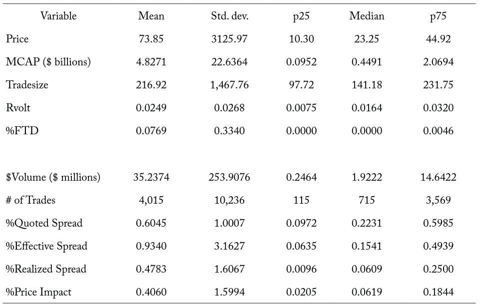
Note: The table reports average daily summary statistics for sample securities in the 40 days prior to the change to a T+2 settlement cycle on September 5, 2017. Price is the closing share price. MCAP is the market capitalization, or closing price times shares outstanding (in billions of dollars). Tradesize is the average number of shares executed in the  . Rvolt is the log of the daily high ask price minus the log of the daily low bid price. %FTD is the percent of share volume that failed to deliver. $Volume is the share volume multiplied by the closing price (in millions of dollars). # of Trades is the total number of trades. During the time interval the %QuotedSpread is defined as
  , where
  is the NBO,
  is the NBB, and
  is the midpoint between the NBBO quotes. %EffectiveSpread is defined as
  where
where  is an indicator variable that equals one if the trade is a buy and minus one if the trade is a sell (the Lee and Ready 1991 algorithm is used to determine trade direction),
  is the price of the trade, and
  is the midpoint of the NBBO quotes assigned to the trade. %RealizedSpread is defined as
  , where is the price of the trade,
  is the NBBO midpoint five minutes after the trade, and is the midpoint of the NBBO quotes assigned to the trade. %PriceImpact is defined as
  , where is the NBBO midpoint five minutes after the trade and is the midpoint of the NBBO quotes assigned to the trade.
In Table 2, we report the pooled Pearson correlation coefficients for the outcome liquidity variables used in the empirical analysis. We show that $Volume and # of Trades carry a positive correlation coefficient of 0.6440. Consistent with previous literature (McInish and Wood 1992), we find an inverse relation between trading activity and bid-ask spreads. Specifically, the correlation coefficient for # of Trades and %Quoted Spread is −0.1864, which is significant at the 0.01 level. However, the remaining correlation coefficients for bid-ask spreads and trading activity are low enough to suggest that we are capturing different dimensions of liquidity. We also note that the %Quoted Spread and %Effective Spread are highly positively correlated (correlation coefficient = 0.4120; p-value = <0.0001). This is not surprising as both measures are intended to proxy a security’s transaction costs. Both %Realized Spread and %Price Impact have high positive correlations with %Effective Spread 0.8243 and 0.8216, respectively.
Table 2. Pooled Pearson correlation coefficients of liquidity measures
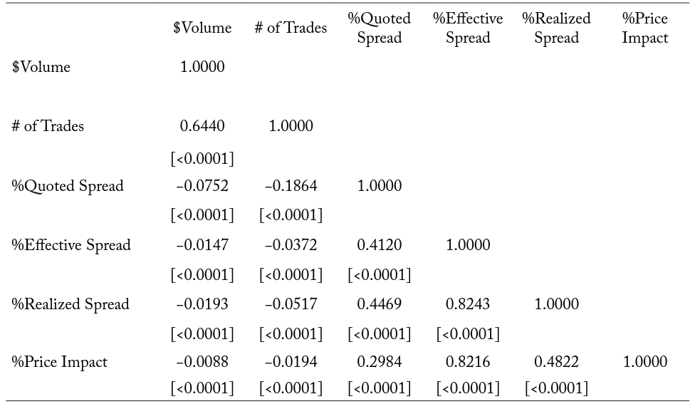
Note: The table reports pooled Pearson correlation coefficients for the liquidity outcome variables in the empirical analysis. The sample includes daily security observations for the 40 days prior to the change to a T+2 settlement cycle on September 5, 2017. $Volume is the share volume multiplied by the closing price (in millions of dollars). # of Trades is the total number of trades. During the time interval the %QuotedSpread is defined as , where is the NBO, is the NBB, and is the midpoint between the NBBO quotes. %EffectiveSpread is defined as where is an indicator variable that equals one if the trade is a buy and minus one if the trade is a sell (the Lee and Ready 1991 algorithm is used to determine trade direction), is the price of the trade, and is the midpoint of the NBBO quotes assigned to the trade. %RealizedSpread is defined as , where is the price of the trade, is the NBBO midpoint five minutes after the trade, and is the midpoint of the NBBO quotes assigned to the trade. %PriceImpact is defined as , where is the NBBO midpoint five minutes after the trade and is the midpoint of the NBBO quotes assigned to the trade.
4. Empirical Results
4.1 T+2 settlement cycle and liquidity
We begin our empirical analysis by examining whether the change in settlement cycle from T+3 to T+2 affects firm-level liquidity. To do so, we estimate specifications of the following fixed-effects regression equation on security-day observations:
(5) 
where the dependent variable is set to one of the following j measures of liquidity: Ln($Volume), Ln(# of Trades), %Quoted Spread, %Effective Spread, %Realized Spread, and %Price Impact. Post is an indicator variable equal to one if the observation is within 40 days after the change to a T+2 settlement cycle on September 5, 2017, and zero for the 40 days before the change. Because of skewness in the data, we take the natural logs of $Volume, # of Trades, Price, MCAP, and Tradesize. We also include day fixed effects (δ ) and security fixed effects (τ ). We report in parentheses -statistics obtained from robust standard errors clustered at the security level.
Table 3. Liquidity around the time of the change to a T+2 settlement cycle
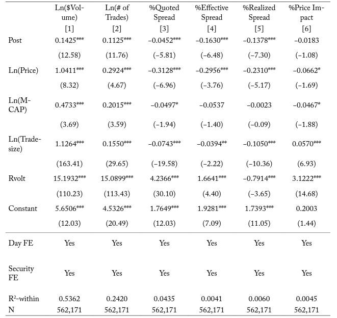
Note: The table reports the regression coefficients from the following equation on daily security observations in the 81-day event window surrounding the change to a T+2 settlement cycle on September 5, 2017:
![\[\operatorname{LIQ}_{i, t}^j=\alpha+\beta_1 \text { Post }_t+\beta_2 \operatorname{Ln}\left(\text { Price }_{i, t}\right)+\beta_3 \operatorname{Ln}\left(M C A P_{i, t}\right)+\beta_4 \operatorname{Ln}\left(\text { Tradesize }_{i, t}\right)+\beta_5 \operatorname{Ln}\left(\text { Rvolt }_{i, t}\right)+\delta_t+\tau_i+\varepsilon_{i, t}\]](https://www.thecgo.org/wp-content/ql-cache/quicklatex.com-050c2f678ee2753f966d98dd48b5fa99_l3.svg "Rendered by QuickLaTeX.com")
where the dependent variable is one of the following  measures of liquidity: $Volume, # of Trades, %Quoted Spread, %Effective Spread, %Realized Spread, and %Price Impact. Post is an indicator variable equal to one if the observation is at the time of or after the change and zero otherwise. We include the following as control variables: Price is the closing share price. MCAP is the market capitalization, or closing price times shares outstanding. Tradesize is the average number of shares executed in a given trade. Rvolt is the log of the daily high ask price minus the log of the daily low bid price. We also include both day fixed effects and security fixed effects. We report in parentheses t-statistics obtained from robust standard errors clustered at the security level. ***, **, and * denote statistical significance at the 0.01, 0.05, and 0.10 levels, respectively.
Consistent with the market-microstructure literature, we find that share price, market capitalization, and trading volume are negatively correlated with percentage spreads.
In columns [1] and [2] of Table 3, we report the results of estimating equation (5) where the dependent variable is set to either Ln($Volume) or Ln(# of Trades). We find that a shortened settlement cycle is associated with a 14.25 percentage-point increase in dollar volume for the average security-day, which translates to over $5 million ($35,237,429 x 0.1425 = $5,021,334). Furthermore, the shortened settlement cycle is associated with an 11.25 percentage-point increase in the number of trades for the average security-day, which equates to over 450 trades (4,015 x 0.1125 = 451.69). To the extent that trading activity is directly related to liquidity, these results indicate that a shortened settlement cycle leads to an improvement in security liquidity, which supports our first hypothesis.
In columns [3] and [4] of Table 3, we display the results of estimating equation (5) where the dependent variable is set to either %Quoted Spread or %Effective Spread. We find that the change in settlement cycle is associated with a 4.52 basis-point decrease in the average %Quoted Spread and a 16.3 basis-point decrease in the average %Effective Spread. In economic terms, these results mean that the cost to trade equities is between 7.5 and 17.5 percent lower after the change. These findings support the notion that a decrease in the settlement cycle is associated with an improvement in security liquidity.
In the final two columns of Table 3, we report the results of estimating equation (5) where the dependent variable is set to either %Realized Spread or %Price Impact. We find that the indicator variable Post is only significant in the model specification in which the outcome variable is %Realized Spread. Specifically, the average %Realized Spread decreases by 13.78 bps after the settlement cycle is reduced, which is a 28.81 percent decrease below pre-event levels. Since the realized spread measures the profitability of liquidity provision, a decrease means that intermediaries might be lowering their fees (the bid-ask spread) because they face lower borrowing constraints. We examine this conjecture further in the following section.
4.2 T+2 settlement cycle and liquidity: borrowing constraints
The results in Table 3 demonstrate that the shortened settlement cycle is associated with improvements in several aspects of security liquidity. In this subsection we examine whether the more difficult-to-borrow securities are driving the results. If intermediaries are truly exposed to lower borrowing constraints after the change to the settlement cycle, we expect to find the largest reductions in trading costs for the more difficult-to-borrow securities.
4.2.1 Market capitalization
Our first proxy for borrowing constraints is average pre-event market capitalization. Geczy, Musto, and Reed (2002) show that small-cap securities are associated with higher lending fees than large-cap securities. Therefore, we rank securities into quartiles based on their average pre-event MCAP, where Q1 refers to small-cap securities (hardest to borrow) and Q4 refers to large-cap securities (easiest to borrow). We then estimate specifications of the following regression equation on security-day observations:
(6) 
where the dependent variable is set to one of the following j measures of liquidity: Ln($Volume), Ln(# of Trades), %Quoted Spread, %Effective Spread, %Realized Spread, and %Price Impact. Post is an indicator variable equal to one if the observation is within the 40 days after the change to a T+2 settlement cycle and zero for the 40 days before the change. 
 are indicator variables equal to one if the security is in the first, second, or third quartiles of the average pre-event market capitalization sample distribution and zero otherwise. Since we include security fixed effects, to avoid violating the full-column-rank assumption for consistent estimation we do not include the individual indicator variables. For this same reason, we also exclude the interaction term between
  and Post. Therefore, the remaining interaction terms are interpreted relative to securities in . We include day fixed effects and report in parentheses -statistics obtained from robust standard errors clustered at the security level. For brevity, we only report the estimated coefficients for the interaction terms.
Table 4. Liquidity around the time of the change to a T+2 settlement cycle by market-capitalization quartiles
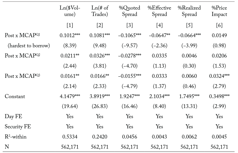
Note: The table reports the regression coefficients from the following equation on daily security observations in the 81-day event window surrounding the change to a T+2 settlement cycle on September 5, 2017:
![\[<span style="font-size: .75em;">L I Q_{i, t}^j=\alpha+\beta_1 \text { Post }_t+\beta_2 M C A P_i^{Q 1}+\beta_3 M C A P_i^{Q 2}+\beta_4 M C A P_i^{Q 3}+\beta_5 \text { Post }_t \times M C A P_i^{Q 1}+\beta_6 \text { Post }_t \times M C A P_i^{Q^2}+\beta_7 \text { Post }_t \times M C A P_i^{Q^3}+\beta_8 \text { Ln }\left(\text { Price }_{i, t}\right)+\beta_9\operatorname{Ln}\left(\text { Tradesize }_{i, t}\right)+\beta_{10} \text { Rvolt }_{i, t}+\delta_t+\tau_i+\varepsilon_{i, t}</span>\]](https://www.thecgo.org/wp-content/ql-cache/quicklatex.com-35e8ce95d56b9b02370a152029449d8a_l3.svg "Rendered by QuickLaTeX.com")
where the dependent variable is one of the following j measures of liquidity: $Volume, # of Trades, %Quoted Spread, %Effective Spread, %Realized Spread, and %Price Impact. Post is an indicator variable equal to one if the observation is at the time of or after the change and zero otherwise. MCAPQx is an indicator variable equal to one if the security is in the first, second, or third quartiles of the pre-event market-capitalization sample distribution and zero otherwise. We exclude the indicator variable MCAPQ4, which is equal to one if the security is in the fourth quartile of preevent market capitalization and zero otherwise, so as to not violate the full-column-rank assumption for consistent estimation. Securities in the first quartile of pre-event market capitalization are estimated to be the most difficult to borrow. We include the following as control variables: Price is the closing share price. Tradesize is the average number of shares executed in a given trade. Rvolt is the log of the daily high ask price minus the log of the daily low bid price. We also include both day fixed effects and security fixed effects. For brevity, we only report the coefficients for the interaction terms. We report in parentheses t-statistics obtained from robust standard errors clustered at the security level. ***, **, and * denote statistical significance at the 0.01, 0.05, and 0.10 levels, respectively.
In columns [1] and [2] of Table 4, we find that the increase in trading activity around the change in settlement cycle is more pronounced for small-cap securities than for large-cap securities. Specifically, the average $Volume (# of Trades) for securities in  increases by 10.12 (10.81) percentage points more than for securities in after the change in settlement cycle. The average $Volume (# of Trades) for securities in
  increases by 2.11 (3.26) percentage points more than for securities in after the change. The average $Volume (# of Trades) for securities in
  increases by 1.61 (1.66) percentage points more than for securities in after the change. Therefore, if a security’s market capitalization proxies borrowing constraints, the smaller and more difficult-to-borrow securities experience a greater increase in trading activity after the change.
In columns [3] and [4] of Table 4, we find that average transaction costs decrease more for small-cap securities than for large-cap securities around the time of the change in the settlement cycle. The average %Quoted Spread narrows by 10.65 bps more for securities in than for securities in after the change. In comparison, the average %Quoted Spread narrows by 2.78 (1.55) bps more for securities in ( ) than for securities in after the change. The average %Effective Spread decreases by 6.47 bps more for securities in 1 than for securities in after the change. We do not find significant differences in changes in percent effective spreads between securities in and those in around the time of the change. Therefore, the smaller and more difficult-to-borrow securities experience a larger decrease in transaction costs around the time of the change.
In columns [5] and [6] of Table 4, we find that the larger decrease in %Effective Spread for small-cap securities relative to large-cap securities around the time of the change is a result of reduced market-making profitability and not reduced price impact. Specifically, we show that the average %Realized Spread decreases by 6.64 bps more for securities in than for securities in after the change. We do not find significant coefficients for the interaction terms when the dependent variable is %Price Impact.
To the extent that a security’s market capitalization proxies its borrowing constraints, our results suggest that the smaller and more difficult-to-borrow securities exhibit greater reductions in transaction costs, and greater increases in trading activity, after the settlement cycle is altered. Thus, intermediaries seem to reduce their spreads more for the hard-to-borrow securities with a shortened settlement cycle, presumably because they have quicker access to funds (and securities) following trade executions, which supports our first hypothesis.
4.2.2 Range volatility
Our second proxy for borrowing constraints is volatility, which is intended to capture investor dispersion. Securities that have high investor dispersion exhibit higher borrowing costs (D’Avolio 2002). Therefore, we sort our sample of securities into quartiles based on their average pre-event  , where Q1 refers to securities in the lowest Rvolt quartile (easiest to borrow) and Q4 refers to securities in the highest quartile (hardest to borrow). We then estimate specifications of the following regression equation on security-day observations:
(7) 
where the dependent variable is set to one of the following j measures of liquidity: Ln($Volume), Ln(# of Trades), %Quoted Spread, %Effective Spread, %Realized Spread, and %Price Impact. Post is an indicator variable equal to one if the observation is within 40 days after the change to a T+2 settlement cycle and zero for the 40 days before the change.  are indicator variables equal to one if the security is in the second, third, or fourth quartile of the average pre-event volatility distribution and zero otherwise. To not violate the full-column-rank assumption for consistent estimation, since we include security fixed effects we do not include the individual indicator variables. For the same reason, we also exclude the interaction term between and
  . Therefore, the remaining interaction terms are interpreted relative to the least volatile securities. We include day fixed effects and report in parentheses
![t\ )-statistics obtained from robust standard errors clustered at the security level. For brevity, we only report the estimated coefficients for the interaction terms. <strong>Table 5. Liquidity around the time of the change to a T+2 settlement cycle by range-volatility quartiles</strong> <a href="https://www.thecgo.org/research/settling-down/screen-shot-2023-07-07-at-5-00-59-pm/" rel="attachment wp-att-19952"><img class="size-full wp-image-19952 aligncenter" src="https://www.thecgo.org/wp-content/uploads/2020/02/Screen-Shot-2023-07-07-at-5.00.59-PM.png" alt="" width="1034" height="612" /></a> <span style="font-size: .75em;">Note: The table reports the regression coefficients from the following equation on daily security observations in the 81-day event window surrounding the change to a T+2 settlement cycle on September 5, 2017:</span> <span class="ql-right-eqno"> </span><span class="ql-left-eqno"> </span><img src="https://www.thecgo.org/wp-content/ql-cache/quicklatex.com-e1f02b9af285eb07dcd218554e4226e2_l3.svg" height="25" width="1819" class="ql-img-displayed-equation " alt="\[<span style="font-size: .75em;">\operatorname{LIQ}_{i, t}^j=\alpha+\beta_1 \text { Post }_t+\beta_2 \text { Rvolt }_i^{Q 2}+\beta_3 \text { Rvolt }_i^{Q 3}+\beta_4 \text { Rvolt }_i^{Q 4}+\beta_5 \text { Post }_t \times \text { Rvolt }_i^{Q 2}+\beta_6 \text { Post }_t \times \text { Rvolt }_i^{Q 3}+\beta_7 \text { Post }_t \times \text { Rvolt }_i^{Q 4}+\beta_8 \operatorname{Ln}\left(\text { Price }_{i, t}\right)+\beta_g \operatorname{Ln}\left(M C A P_{i, t}\right)+\beta_{10} \operatorname{Ln}\left(\text { Tradesize }_{i, t}\right)+\delta_t+\tau_i+\varepsilon_{i, t}</span>\]" title="Rendered by QuickLaTeX.com"/> <span style="font-size: .75em;">where the dependent variable is one of the following \(j](https://www.thecgo.org/wp-content/ql-cache/quicklatex.com-ede4a9fc0d8907d36d5c67f66f6648b9_l3.svg "Rendered by QuickLaTeX.com")
measures of liquidity: $Volume, # of Trades, %Quoted Spread, %Effective Spread, %Realized Spread, and %Price Impact. Post is an indicator variable equal to one if the observation is at the time of or after the change and zero otherwise.  is an indicator variable equal to one if the security is in the second, third, or fourth quartiles of the average pre-event range-volatility sample distribution and zero otherwise. We exclude the indicator variable
  , which is equal to one if the security is in the first quartile of pre-event average range volatility and zero otherwise, so to not violate the full-column-rank assumption for consistent estimation. Securities in the fourth quartile of pre-event average range volatility are estimated to be the most difficult to borrow. We include the following as control variables: Price is the closing share price. MCAP is the market capitalization, or closing price times shares outstanding. Tradesize is the average number of shares executed in a given trade. We also include both day fixed effects and security fixed effects. For brevity, we only report the coefficients for the interaction terms. We report in parentheses t-statistics obtained from robust standard errors clustered at the security level. ***, **, and * denote statistical significance at the 0.01, 0.05, and 0.10 levels, respectively.
In columns [1] and [2] of Table 5, we show that the increase in trading activity around the time of the change to the settlement cycle is directly related to a security’s average pre-event volatility. For instance, the average $Volume (# of Trades) for securities in increases by 6.48 (5.62) percentage points more than for securities in after the change. We also find that average $Volume increases more for securities in (1.73 percentage points) and (2.13 percentage points) than for securities in after the change. We do not find that the changes in average # of Trades differ significantly between volatility quartiles one through three. To the extent that volatility proxies borrowing constraints, our results indicate that the more volatile and difficult-to-borrow securities experience a greater increase in trading activity after the settlement cycle is shortened.
In columns [3] and [4] of Table 5, we find that the lower trading costs associated with the shortened settlement cycle are more pronounced for securities with higher average pre-event volatility than those with lower average pre-event volatility. Specifically, we find that the average %Quoted Spread narrows by 12.49 bps more for securities in than for securities in after the change. Additionally, we show that the average %Effective Spread decreases by 10.54 bps more for securities in than for securities in after the change. Therefore, the T+2 settlement cycle seems to reduce transaction costs most for the more volatile and difficult-to-borrow securities.
We only find one significant coefficient for the interaction terms in columns [5] and [6] of Table 5, where the dependent variable in equation (7) is either %Realized Spread or %Price Impact. Specifically, we find that the average %Realized Spread decreases by 8.42 bps more for securities in than for securities in after the change in the settlement cycle. We do not find significant differences between volatility quartiles when %Price Impact is the outcome variable. Again, these results suggest that any change in transaction costs around the time of the change is a result of decreasing market-making profits.
To the extent that return volatility at least partially captures borrowing constraints, our results suggest that the volatile and more difficult-to-borrow securities experience a greater increase in liquidity (higher trading activity and lower transaction costs) after the settlement cycle is shortened. Similar to the results in section 4.2.1, these findings lend support to our first hypothesis.
4.2.3 Failures to deliver
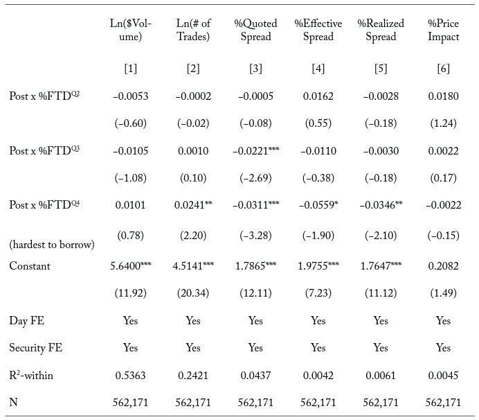
Our third proxy for borrowing constraints is failures to deliver. Securities with more failures to deliver are considered hard to borrow given their high short-sale constraints and high loan fees (Autore, Boulton, and Braga-Alves 2015). Similar to before, we sort our sample of securities into quartiles by average pre-event  , where Q1 refers to securities in the lowest quartile (easiest to borrow) and Q4 refers to securities in the highest quartile (hardest to borrow). We then estimate specifications of the following regression equation on security-day observations:
(8) 
where the dependent variable is set to one of the following j measures of liquidity: Ln($Volume), Ln(# of Trades), %Quoted Spread, %Effective Spread, %Realized Spread, and %Price Impact. is an indicator variable equal to one if the observation is within the 40 days after the change to the T+2 settlement cycle and zero for the 40 days before the change. are indicator variables equal to one if the security is in the second, third, or fourth quartile of the average pre-event (\%FTD\)sample distribution and zero otherwise. To not violate the full-column-rank assumption for consistent estimation, since we include security fixed effects we do not include the individual indicator variables. We also exclude the interaction between and . Therefore, the interaction terms are interpreted relative to securities with the fewest failures to deliver. We include day fixed effects and report in parentheses -statistics obtained from robust standard errors clustered at the security level. For brevity, we only report the estimated coefficients for the interaction terms.
Table 6. Liquidity around the time of the change to a T+2 settlement cycle by percent failure-to-deliver quartiles
Note: The table reports the regression coefficients from the following equation on daily security observations in the 81-day event window surrounding the change to a T+2 settlement cycle on September 5, 2017:
![\[<span style="font-size: .75em;">L I Q_{i, t}^j=\alpha+\beta_1 \operatorname{Post}_t+\beta_2 \% F T D_i^{Q^2}+\beta_3 \% F T D_i^{Q^3}+\beta_4 \% F T D_i^{Q^4}+\beta_5 \text { Post }_t \times \% F T D_i^{Q^2}+\beta_6 \text { Post }_t \times \% F T D_i^{Q^3}+\beta_7 \text { Post }_t \times \% F T D_i^{Q^4}+\beta_s \operatorname{Ln}\left(\text { Price }_{i, t}\right)+\beta_9 \operatorname{Ln}(M-\text { CAP } \left.\left._{i, t}\right)+\beta_{10} \operatorname{Ln}\left(\text { Tradesize }_{i, t}\right)+\beta_{11} \text { Rvolt }_{i, t}\right)+\delta_t+\tau_i+\varepsilon_{i, t}</span>\]](https://www.thecgo.org/wp-content/ql-cache/quicklatex.com-8b843abaaff6b70b14c3c6a89e054022_l3.svg "Rendered by QuickLaTeX.com")
where the dependent variable is one of the following measures of liquidity: $Volume, # of Trades, %Quoted Spread, %Effective Spread, %Realized Spread, and %Price Impact. Post is an indicator variable equal to one if the observation is at the time of or after the change and zero otherwise. %FTDQx is an indicator variable equal to one if the security is in the second, third, or fourth quartiles of the average pre-event percent failures-to-deliver sample distribution and zero otherwise. We exclude the indicator variable %FTDQ1, which is equal to one if the security is in the first quartile of pre-event percent failures to deliver and zero otherwise, so as to not violate the full-column-rank assumption for consistent estimation. Securities in the fourth quartile of pre-event percent failures to deliver are estimated to be the most difficult to borrow. We include the following as control variables: Price is the closing share price. MCAP is the market capitalization, or closing price times shares outstanding. Tradesize is the average number of shares executed in a given trade. Rvolt is the log of the daily high ask price minus the log of the daily low bid price. We also include both day fixed effects and security fixed effects. For brevity, we only report the coefficients for the interaction terms. We report in parentheses t-statistics obtained from robust standard errors clustered at the security level. ***, **, and * denote statistical significance at the 0.01, 0.05, and 0.10 levels, respectively.
In columns [1] and [2] of Table 6, we find that trading activity increases more for securities with high pre-event\ (%FTD\) than for securities with low pre-event after the change in the settlement cycle. However, the change in average $Volume around the time of the change in the cycle is not different between securities in and securities in . The average # of Trades increases by 2.41 percentage points more for securities in than for securities in after the change. If (%FTD\) is an adequate proxy for borrowing constraints, our results indicate that harder-to-borrow securities experience a greater increase in trading activity, at least in terms of # of Trades, after the change. We also find, in columns [3] through [6] of Table 6, that transaction costs decrease more for securities with high pre-event than for securities with low pre-event after the change. More specifically, the average %Quoted Spread (%Effective Spread) narrows by 3.11 (5.59) bps more for securities in than for securities in . Furthermore, the average %Realized Spread decreases by 3.46 bps more for securities in\ (%FTD\) than for securities in . We do not find significant differences in the change in %Price Impact between (%FTD\) quartiles around the time of the change. Since securities with high present larger borrowing risks to intermediaries than those with low (\%FTD\), our results here indicate that liquidity improves more for difficult-to-borrow securities around the time of the change in the settlement cycle. As in sections 4.2.1 and 4.2.2, these results provide further support for our first hypothesis.
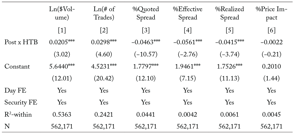
4.2.4 Hard-to-borrow securities Our final proxy for borrowing constraints is obtained from a list of easy-to-borrow securities compiled by MB Trading.10The complete list of easy-to-borrow securities is available at http://www.mbtrading.com/easyToBorrow.aspx. Note that this list does not align with our sample period. The brokerage firm states that the list comprises securities that are available to short sell. We then create a categorical variable, HTB, that equals one if the security is not on MB Trading’s list and zero if it is on the list. We then estimate the following regression equation on security-day observations:
(9) 
where the dependent variable is set to one of the following j measures of liquidity: Ln($Volume), Ln(# of Trades), %Quoted Spread, %Effective Spread, %Realized Spread, and %Price Impact. is an indicator variable equal to one if the observation is within 40 days after the change to the T+2 settlement cycle and zero for the 40 days before the change. The interaction term between and HTB is the difference-in-difference estimator. To avoid violating the full-column-rank assumption for consistent estimation, since we include security fixed effects we do not include the firm-invariant HTB indicator variable. The control variables are defined in section 3.2. We include day fixed effects and report in parentheses -statistics obtained from robust standard errors clustered at the security level. For brevity, we only report the estimated coefficient for the interaction term.
Table 7. Liquidity around the time of the change to a T+2 settlement cycle by hard-to-borrow securities
Note: The table reports the regression coefficients from the following equation on daily security observations in the 81-day event window surrounding the change to a T+2 settlement cycle on September 5, 2017:
![\[<span style="font-size: .75em;">\left.\left.L I Q_{i, t}^j=\alpha+\beta_1 \text { Post }_t+\beta_2 H_{T B_i}+\beta_3 \text { Post }_t \times H T B_i+\beta_4 \text { Ln }^{\text {Lrice }}{ }_{i, t}\right)+\beta_5 \operatorname{Ln}\left(M C A P_{i, t}\right)+\beta_6 \text { Ln } \text { Tradesize }_{i, t}\right)+\beta_7 \text { Rvolt }_{i, t}+\delta_t+\tau_i+\varepsilon_{i, t}</span>\]](https://www.thecgo.org/wp-content/ql-cache/quicklatex.com-28ad136c92da0601e84c5ccfdc4348f1_l3.svg "Rendered by QuickLaTeX.com")
where the dependent variable is one of the following j measures of liquidity: $Volume, # of Trades, %Quoted Spread, %Effective Spread, %Realized Spread, and %Price Impact. Post is an indicator variable equal to one if the observation is at the time of or after the change and zero otherwise. HTB is an indicator variable equal to one if the security is not on MB Trading’s easy-to-borrow security list and zero if it is on the list. We include the following as control variables: Price is the closing share price. MCAP is the market capitalization, or closing price times shares outstanding. Tradesize is the average number of shares executed in the  trade. Rvolt is the log of the daily high ask price minus the log of the daily low bid price. We also include both day fixed effects and security fixed effects. For brevity, we only report the coefficient for the interaction terms. We report in parentheses t-statistics obtained from robust standard errors clustered at the security level. ***, **, and * denote statistical significance at the 0.01, 0.05, and 0.10 levels, respectively.
In the first two columns of Table 7, we find that after the change in the settlement cycle, average trading activity increases significantly more for securities that are hard to borrow than for those that are easy to borrow. For example, the average $Volume increases by 2.05 percentage points more for securities that are hard to borrow than for securities that are easy to borrow. Similarly, the average # of Trades increases by 2.98 percentage points more for securities that are hard to borrow than for those that are easy to borrow. These results lend further support to the notion that the more difficult-to-borrow securities experience a greater increase in liquidity.
We show, in columns [3] and [6] of Table 7, that after the settlement cycle is shortened, average trading costs decrease more for securities that are hard to borrow than for securities that are easy to borrow. Specifically, the average %Quoted Spread, %Effective Spread, and %Realized Spread decrease by 4.63, 5.61, and 4.15 bps, respectively, more for securities that are hard to borrow than for securities that are easy to borrow. As in our previous tests, we do not find significant differences in %Price Impact between hard-to-borrow and easy-to-borrow securities around the time of the change.
Overall, the evidence in section 4.2 provides consistent support for our first hypothesis. For instance, we find that more difficult-to-borrow securities, measured by , , , and  , experience the greatest gains in liquidity after the settlement cycle is shortened. This seems to agree with the SEC (see Release No. 34-80295), which argued ex ante that a shortened settlement cycle would free up capital to financial intermediaries by exposing them to less liquidity risk. Our results suggest that a loosening of financial constraints allows intermediaries to narrow their bid-ask spreads, which in turn attracts more trading activity.
4.3 Robustness: T+3 settlement cycle and liquidity
On June 7, 1995, the SEC approved the transition from a T+5 settlement cycle to a T+3 settlement cycle. As a robustness check, we replicate the majority of our analysis using the change to a T+3 settlement cycle as a natural experiment. Since we do not have access to the more granular NYSE DTAQ database for this sample period, we must rely on a low-frequency proxy for liquidity. We follow Amihud (2002) and measure illiquidity by security-day as the absolute return divided by dollar volume. In unreported results, we find that illiquidity decreases and dollar volume increases more for securities that are hard to borrow (measured by average pre-event and ) than for securities that are easy to borrow after the transition.11We are unable to measure %FTD or HTB as we do not have access to these data during the older sample period. The results from these additional tests provide further support for our first hypothesis that a shortened settlement cycle improves liquidity, particularly for the more difficult-to-borrow securities.12The results from this analysis are available by the authors upon request.
5. Concluding Remarks
On September 5, 2017, the SEC shortened the standard settlement cycle for nearly all broker-dealer equity transactions from T+3 to T+2. In this paper, we examined the effects of the shortened settlement cycle on firm-level liquidity. According to a cost-benefit analysis commissioned by the DTCC and conducted by the Boston Consulting Group (2012), many market participants supported a move to a shortened settlement cycle, citing process efficiency and risk reduction as motivators.
Our results show that the change is associated with a significant improvement in security liquidity. Specifically, we find that bid-ask spreads are narrower and trade volumes are higher in the 40 days following the change. We contend that the decrease in transaction costs provides tangential evidence that intermediaries have faced lower counterparty risks since the rule change, as the fees (e.g., margin charges) that are passed down by market makers to other market participants, including both institutional and retail investors, are lower. The increase in liquidity should allow investors to better manage their portfolios through lower-cost rebalancing and asset reallocation.
The findings in this study also show that securities with tight borrowing constraints experienced the greatest gains in liquidity after the move to a T+2 settlement cycle. These results are robust to various proxies of borrowing constraints (viz., pre-event market capitalization, volatility, failures to deliver, and hard-toborrow securities) and various econometric specifications. Therefore, a shortened settlement cycle seems to reduce the financial collateral needed by broker-dealers and central-counterparty members to facilitate transactions. Consequently, this might reduce asset managers’ exposure to both inventory risk and counterparty-default risk.
In addition to the practical relevance of our findings, our paper has important policy implications as both domestic and global equity markets are considering a move to an even-shorter settlement period. Most international markets have already transitioned to a T+2 settlement cycle, but many are still considering a move to T+1. Our findings indicate that a shortened settlement cycle improves liquidity in US equity markets, particularly for securities that are more difficult to borrow. Fruitful areas for future research might be to generalize our finding to other markets and to examine other aspects of market liquidity and efficiency.
References
Alizadeh, S., M. W. Brandt, and F. X. Diebold. 2002. “Range‐Based Estimation of Stochastic Volatility Models.” Journal of Finance 57 (3): 1047–91.
Amihud, Y. 2002. “Illiquidity and Security Returns: Cross-section and Time-Series Effects.” Journal of Financial Markets 5 (1): 31–56.
Autore, D. M., T. J. Boulton, and M. V. Braga‐Alves. 2015. “Failures to Deliver, Short Sale Constraints, and Security Overvaluation.” Financial Review 50 (2): 143–72.
Boston Consulting Group. 2012. “Shortening the Settlement Cycle.” Discussion paper, Boston Consulting Group.
Branch, B., and W. Freed. 1977. “Bid-Asked Spreads on the AMEX and the Big Board.” Journal of Finance 32 (1): 159–63.
Brunnermeier, M. K., and L. H. Pedersen. 2009. “Market Liquidity and Funding Liquidity.” Review of Financial Studies 22 (6): 2201–38.
Chakrabarty, B., B. Li, V. Nguyen, and R. A. Van Ness. 2007. “Trade Classification Algorithms for Electronic Communications Network Trades.” Journal of Banking & Finance 31 (12): 3806–21.
Comerton‐Forde, C., T. Hendershott, C. M. Jones, P. C. Moulton, and M. S. Seasholes. 2010. “Time Variation in Liquidity: The Role of Market‐Maker Inventories and Revenues.” Journal of Finance 65 (1): 295–331.
Copeland, T. E., and D. Galai. 1983. “Information Effects on the Bid‐Ask Spread.” Journal of Finance 38 (5): 1457–69.
D’avolio, G. 2002. “The Market for Borrowing Security.” Journal of Financial Economics 66 (2–3): 271–306.
Ellis, K., R. Michaely, and M. O’Hara. 2000. “The Accuracy of Trade Classification Rules: Evidence from Nasdaq.” Journal of Financial and Quantitative Analysis 35 (4): 529–51.
Geczy, C. C., D. K. Musto, and A. V. Reed. 2002. “Securities Are Special Too: An Analysis of the Equity Lending Market.” Journal of Financial Economics 66 (2–3): 241–69.
Glosten, L. R., and P. R. Milgrom. 1985. “Bid, Ask and Transaction Prices in a Specialist Market with Heterogeneously Informed Traders.” Journal of Financial Economics 14 (1): 71–100.
Glosten, L. R., and L. E. Harris. 1988. “Estimating the Components of the Bid/Ask Spread.” Journal of Financial Economics 21 (1): 123–42.
Hamilton, J. L. 1978. “Marketplace Organization and Marketability: NASDAQ, the Security Exchange, and the National Market System.” Journal of Finance 33 (2): 487–503.
Holden, C. W., and S. Jacobsen. 2014. “Liquidity Measurement Problems in Fast, Competitive Markets: Expensive and Cheap Solutions.” Journal of Finance 69 (4): 1747–85.
Khapko, M., and M. Zoican. 2018. “Smart Settlement.” Working paper, University of Toronto.
Lee, C. M., and M. J. Ready. 1991. “Inferring Trade Direction from Intraday Data.” Journal of Finance 46 (2): 733–46.
Levitt, A. 1996. “Speeding Up Settlement: The Next Frontier.” Remarks at the US SEC Symposium on Risk Reduction in Payments, Clearance and Settlement Systems. https://www.sec.gov/news/speech/speecharchive/1996/spch071.txt.
McInish, T. H., and R. A. Wood. 1992. “An Analysis of Intraday Patterns in Bid/Ask Spreads for NYSE Securities.” Journal of Finance 47(2): 753–64.
Menkveld, A. J., E. Pagnotta, and M. Zoican. 2015. “Does Central Clearing Affect Price Stability? Evidence from Nordic Equity Markets.” Working paper, VU Amsterdam.
O’Hara, M., and G. S. Oldfield. 1986. “The Microeconomics of Market Making.” Journal of Financial and Quantitative Analysis 21 (4): 361–76.
SEC (Securities and Exchange Commission). 2017. “Securities Transaction Settlement Cycle.” Release no. 34–80295; file no. S7–22–16.
Stoll, H. R. 1978. “The Supply of Dealer Services in Securities Markets.” Journal of Finance 33 (4): 1133– 51.
Stoll, H. R. 1989. “Inferring the Components of the Bid‐Ask Spread: Theory and Empirical Tests.” Journal of Finance 44 (1): 115–34.
Stratmann, T. and Welborn, J.W., 2016. Informed short selling, fails-to-deliver, and abnormal returns. Journal of Empirical Finance 38, pp.81-102.
Tinic, S. M. 1972. “The Economics of Liquidity Services.” Quarterly Journal of Economics 1:79–93.
Tinic, S. M., and R. R. West. 1972. “Competition and the Pricing of Dealer Service in the Over-theCounter Security Market.” Journal of Financial and Quantitative Analysis 7 (3): 1707–17.