On Regional Borrowing, Default, and Migration

Gordon, Grey; Guerron-Quintana, Pablo

Introduction

The local government finances of Detroit and Flint, Michigan, have received significant attention in the media, and for good reason. The two cities have both experienced shrinking populations (with declines exceeding 30% since 1986) and wages (decreasing 10% and 30%, respectively) that have placed significant strain on their finances. Detroit responded to these challenges with burgeoning debt—which grew from $2,000 per person to $12,500 in 2012 dollars—and a default in 2013, while Flint kept debt low but was forced to raise taxes from $3,000 to $4,500 per person. Which of these paths was best? Could anything else have been done? Were these debt levels optimal or too high? Currently, there is scant empirical evidence and no model linking city finances, migration, and default. This paper fills these gaps in the literature in two ways: first, by merging panel datasets on local government finances, labor productivity, and migration to document patterns of cities in general and defaulting cities in particular; and, second, by proposing and analyzing a rich and novel general equilibrium model that successfully captures these patterns.

To guide our investigation of the data, we first consider a comparatively simple two-period islands model of the type used in Lucas (1972). Each island represents a local economy and has (1) a continuum of households who make migration decisions, (2) an exogenously given per person endowment that is location-specific, and (3) a planner who issues debt in the first period (transferring the proceeds to households) and repays it in the second (using lump-sum taxes). The key assumption is that the local planner maximizes the welfare of current residents. The model reveals that, relative to an economy-wide planner, local planners have an incentive to overborrow. The reason is simple: new arrivals in the second period will help repay debt issued in the first period, and the planner does not directly value their utility. There is a potentially offsetting effect, namely, that as borrowing increases, the island’s attractiveness to newcomers declines and this increases debt per person. However, we show that in general equilibrium with two heterogeneous island types, the equilibrium is not constrained efficient—i.e., not efficient taking migration decisions as given—and is therefore not Pareto efficient, either.

The theory suggests that cities should accumulate large amounts of debt, that cities with larger in-migration rates all else equal should accumulate more debt, and that states or federal governments should have policies in place that restrict municipal borrowing. (For our purposes, we will refer to cities and municipalities interchangeably.)¹ Using comprehensive datasets on city finances, population, migration, and labor productivity as well as institutional details, we find support for all of these predictions. Results from fixed effects regressions reveal a positive correlation between deficits and in-migration rates. Moreover, we show many states have restrictions on municipal borrowing. While the form of most of the states’ borrowing limits precludes us from measuring how close cities are to the limits, for California and Michigan we can tell. And there, it seems most cities are close to, at, or even above the limit.

We further look at the relationship between borrowing, migration, and default by conducting a case study of municipal defaults—which are rare overall but have doubled in number since the early 2000s. The study reveals that defaulters have larger debt, expenditures, and deficits than typical cities. However, heterogeneous paths lead to default: defaults have happened during challenging times characterized by population declines and low productivity (as in Detroit and Flint), but also during productivity or population booms (as in San Bernardino, Stockton, and Vallejo, California).² Theoretically, the bust defaults are unsurprising: negative, mean-reverting shocks should result in borrowing for consumption smoothing purposes with persistently negative ones leading to default. However, based on that intuition, the boom defaults are very surprising. Yet, our model offers an explanation: In response to rapid population growth, cities overborrow, expecting future entrants to help repay the debt. Then, with a high amount of leverage, default looks attractive when a negative shock eventually occurs.

We extend the two-period model to capture these empirical regularities, allowing for a decentralized economy with production, government services, housing, borrowing limits, default, and an infinite horizon, as well as a taste shifter we think of as weather. After showing the economy can be centralized (at a local level), we demonstrate the calibrated model is capable of matching a host of statistics including the mean and standard deviation of in- and out-migration rates, mean default rates, interest rates on municipal debt, local debt-to-GDP ratios, the standard deviation of log population, correlations between productivity and migration rates, and population autocorrelations. The model also reproduces the patterns observed in the fixed effects regressions and the proximity of cities to borrowing limits in the cross-section. Importantly, the model generates both boom and bust defaults.

Having established the model’s success in matching relevant features of municipal borrowing, migration, and default, we turn to its counterfactual predictions. Feeding in the estimated productivity process for Detroit—which shows a rapid decline beginning in 2006 and continuing through 2012—gives an alternative, and optimal, path for its economy. The results show, perhaps surprisingly, that Detroit’s debt levels in the early 2000s (around $7,000 per person in 2010 dollars) were nearly optimal. However, when the financial crisis hit, it should have deleveraged by around $750 per person via large cuts to expenditures and smaller cuts to taxes. In contrast, Detroit raised taxes in 2009 and 2010 and expenditures and debt per person rose almost continually from 2006 to 2011, precipitating default.

We also investigate the consequences of three policy changes. First, we look at increasing the risk-free municipal bond interest rate from 4% (its real value in 2010) to 6.5% (its actual value in the early 1990s). We show raising rates causes migration away from high-debt, low-productivity cities to low-debt, high-productivity ones, providing a slight boost to aggregate output but with few other consequences in the long run. Second, we look at elimination of state-imposed borrowing limits. We show this has small effects precisely because private credit markets constrain city borrowing virtually as much as the state-imposed constraints. Finally, we investigate the consequences of bailouts in our calibrated model. We find $\varepsilon$ -bailouts—defined as the smallest transfer sufficient to avoid default—double default rates but otherwise have small effects. The reason is $\varepsilon$ -bailouts are not attractive because (1) they give the same utility as default in the bailout period and, (2) to match both large debt positions and low default rates in the data, the calibration makes default costly (equal to 8.4% of annual income). Hence, while bailouts do create a moral hazard problem and lead to some increase in default rates, the moral hazard is mitigated by low ex post returns from being bailed out.

Since our model features local governments competing (through migration) via taxes and spending, it connects to large literatures on tax competition and fiscal federalism as surveyed by Wilson (1999) and Weingast (2009). In influential work, Tiebout (1956) showed this competition can lead to efficiency, and we show that—in a case where migration reacts to policies in an extreme way—there can be efficiency. Outside of this extreme case, however, we prove the equilibrium is generally inefficient. Interestingly, the inefficiency does not come from either of the two common sources Wilson (1999) highlights.³

A few papers in this literature have discussed the potential for local governments to overborrow because of migration. In particular, Bruce (1995) and Schultz and Sjöström (2001) prove that overborrowing generally does occur. However, both of their models are two-period, partial equilibrium models with costless moving. And, in fact, we show that the Bruce (1995) and Schultz and Sjöström (2001) results need not go through in general equilibrium: with symmetry, general equilibrium bond prices undo the incentive to overborrow. (But overborrowing does occur with a modicum of heterogeneity.) More importantly, we contribute to this literature by showing empirically and quantitatively the role of overborrowing in reproducing many of the data’s features.

Our paper also builds on the large sovereign default literature begun by Eaton and Gersovitz (1981), which has focused almost exclusively on nation states.⁴ Epple and Spatt (1986) is an exception that argues states should restrict local debt because default by one local government makes other local governments appear less creditworthy. Such a force is not at work in our model because we assume full information. We contribute to this literature by showing migration strongly influences debt accumulation and can result in boom defaults.

Our work also connects to a vast literature on intranational migration. The empirical work and to a lesser extent theoretical is surveyed in Greenwood (1997). Two seminal papers in this literature, Rosen (1979) and Roback (1982), employ a static model with perfectly mobile labor. This implies every region provides individuals with the same utility. While this indifference condition allows for elegant characterizations of equilibrium prices and rents, it also means government policies are completely indeterminate: every debt, service, or tax choice results in the same utility. Our model breaks this result by assuming labor is imperfectly mobile, which lets it match both the sluggish population adjustments and the small correlations between productivity and migration rates observed in the data.

More recently, Armenter and Ortega (2010), Coen-Pirani (2010), Van Nieuwerburgh and Weill (2010), Kennan and Walker (2011), Davis, Fisher, and Veracierto (2013), and Caliendo, Parro, Rossi-Hansberg, and Sarte (2017) have analyzed determinants of migration and its consequences in the U.S. Kennan and Walker (2011) use a structurally estimated model of migration decisions and find expected income differences play a key role, providing external evidence of the model’s productivity-driven migration decisions. Outside the U.S., much recent research has been focused on migration in the European Union (Kennan, 2013, 2017; Farhi and Werning, 2014). All these papers abstract from debt. To our knowledge, there are no other published quantitative models of regional borrowing and migration, let alone any having default.

On borrowing and migration

Before turning to the data, we highlight how migration influences borrowing decisions and efficiency using a two-period model. To focus purely on the role of borrowing, we assume there is full commitment to repay debt and, hence, no default.
The economy is comprised of a unit measure of islands and a unit measure of households. Consider an arbitrary island. In the first (second) period, the island has a per person nonstochastic endowment of $y_1$ $(y_2)$ . The local planner / government issues $-b_2$ debt per person ( $b_2 > 0$ means assets) at price $\overline{q}$ . Total debt issuance is $-b_2n_1$ , where $n_1$ is the initial measure of households on the island. At the beginning of the second period, households draw an idiosyncratic utility cost of moving $\phi ~ F(\phi)$ with a density $f$ and then decide whether to migrate. If they migrate, they pay $\phi$ and obtain expected utility $J$ , which is an equilibrium object.

Households value consumption according to $u(c_1) + \betau(c_2)$ , where $c_1 (c_2)$ is consumption in the first (second) period. Household utility in the second period is $u(c_2)$ if they stay and $J - \phi$ if they move, so migration decisions follow a cutoff rule in $\phi$ with indifference at $J - u(c_2)$ . Consequently, the outflow rate is $o_2 = F(J - u(c_2))$ . The inflow rate is given by $i_2 = \overline{i}I(u(c_2))$ , where I is a differentiable, increasing function and $\overline{i}$ is an equilibrium object that ensures aggregate inflows equal aggregate outflows. (Consequently, inflows can depend on the distribution of utility across islands, but that information must be summarized in $\overline{i}$ .) The population law of motion is $n_2 = (1 + i_2 - o_2)n_1$ . We assume the migration decision is noisy in the sense that $F(0) > 0$ , so that some people will move even if $u(c_2) = J$ .⁵

After all migration has taken place, the government pays back its total obligation, $-b_2n_1$ , by taxing the $n_2$ households lump sum. Consequently, per person consumption in the second period is $c_2 = y_2 + b_2_n1/n_2$ . The government’s problem may be written

(1) $\begin{equation*} \begin{gathered} max_{b2} u(c_1) + \beta \int max \left\{u(c_2), J - \phi \right\} dF(\phi) \\ s.t. c_1 + \overline{q}b_2 = y_1, c_2 = y_2 + b_2 \frac{n_1}{n_2}, n_2 = n_1(1 - o_2 + i_2), c_1, c_2 \ge 0, \\ i_2 = \overline{i}I(u(c_2)), o_2 = F(J - u(c_2)). \end{gathered} \end{equation*}$

Proposition 1 gives the Euler equation for government bonds (all proofs are in Appendix D).

Proposition 1. The local government’s Euler equation is

(2) $\begin{equation*} \begin{gathered} u^{\prime} (c_1)\overline{q} = \beta \frac{1 - o_2}{1 - o_2 + i_2} u^{\prime}(c_2) (1 − \frac{b_2}{n_2} \frac{\partial n_2}{\partial b_2}) \end{gathered} \end{equation*}$

The Euler equation reflects two competing forces. One is an externality seen in the term $\frac{1- o_2} {1-o_2+i_2} \le 1$ . Because the planner does not value the utility of new entrants and because new entrants bear $\frac{i_2}{1-o_2+i_2}$ of the debt burden (which is their share of the second-period population), the marginal cost associated with an additional unit of debt—holding fixed migration rates—is 1 − $\frac{i_2}{1-o_2+i_2}$ or $\frac{1-o_2}{ 1-o_2+i_2}$ . All else equal, higher in-migration lowers the effective discount factor $(\beta \frac{1-o_2}{ 1-o_2+i2} )$ and increases borrowing. Clearly, then, the assumption that the planner only values current residents plays a key role. But note that is also the most natural assumption: if current residents could vote on the planner’s policy in the first period, they would unanimously approve it because it maximizes their welfare.

The other force is seen in the term $1 − \frac{b_2}{n_2} \frac{\partial n_2} {\partial b_2}$ , which is one minus the elasticity of the next period’s population with respect to savings. It reflects that for each person attracted to the island through less borrowing, the overall debt burden per person falls. (Conversely, if $b_2 > 0$ , each additional entrant reduces assets per person, which discourages savings.) Hence, a rational government, internalizing the effects of city finances on migration decisions, should exercise more financial discipline all else equal to attract individuals to their island and thus reduce debt per person.

Consider two equilibrium concepts. A closed economy equilibrium is a 3-tuple { $\overline{i}, J, \overline{q}$ } with optimal migration, consumption, and borrowing decisions such that

total inflows equal total outflows, $\overline{i} \int I(u(c_{2,j} ))n_{1,j}dj = \int F(J - u(c_{2,j} ))n_{1,j}dj;$
the expected utility of moving is consistent, $J = \int u(c_{2,j} ) \frac{\overline{i}I(u(c_{2,j} ))n_{1,j}} { \int \overline{i}I(u(c_{2,i}))n_{1,i}di}dj$ ; and
the bond market is in zero net supply, $\int b_{2,j}n_{1,j}dj = 0$ .

An open economy equilibrium differs in that $\overline{q}$ is taken parametrically and the bond market clearing is not required.

Is the equilibrium optimal from a societal perspective? To answer this, we need a social planner problem. To this end, let $\hat{c}_{1,i}$ , $\hat{c}_{2,i}$ denote the optimal consumption (in periods 1 and 2, respectively) of household $i \in [0, 1]$ , and let $\phi_i$ denote the moving cost shock realization the household receives. Let $y_{1,i}$ denote the endowment agent $i$ will receive in the first period (which depends on their initial island placement). Similarly, let $y^{s}_{2,i}$ denote the output the household will receive if she decides to stay on her island and $\overline{y}^{m}_{2,i}$ the output in expectation associated with its moving. Taking migration decisions as given, the planner’s objective function is

(3) $\begin{equation*} \begin{gathered} max\limits_{\hat{c}_{1,i} \ge 0, \hat{c}_{2,i}\ge 0} \int \alpha (u(\hat{c}_{1,i}) + \beta(u(\hat{c}_{2,i}) − m_i \phi_i))di \end{gathered} \end{equation*}$

where $\alpha_i$ is the Pareto weight on household $i$ . We will consider two formulations of the resource constraint, an open economy resource constraint given by

(4) $\begin{equation*} \begin{gathered} \int \hat{c}_{1,i} di + \hat{q} \int \hat{c}_{2,i} di = \int y_{1,i} di + \hat{q} \int ((1 − m_i)y^{s}_{2,i} + m_i\overline{y}^{m}_{2,i})di \end{gathered} \end{equation*}$

and a closed economy resource constraint given by

(5) $\begin{equation*} \begin{gathered} \int \hat{c}_{1,i} di = \int y_{1,i} di and \int \hat{c}_{2,i} di = \int ((1 − m_i)y^{s}_{2,i} + m_i\overline{y}^{m} _{2,i})di. \end{gathered} \end{equation*}$

If the planner can choose migration decisions, then $m_i \in [0, 1]$ should be added as a choice variable and $\overline{y}^{m}_{2,i}$ will be identically equal to the maximum second-period endowment value.⁶

Definition 1. An allocation is constrained efficient if it solves the planner problem with migration decisions given for some Pareto weights.

For either resource constraint, optimality requires that marginal rates of substitution must be equated across individuals, i.e., $\beta u^{\prime} (\hat{c}_{2,i})/u^{\prime}(\hat{c}_{1,i}) = \beta u^{\prime} (\hat{c}_{2,j})/u^{\prime} (\hat{c}_{1,j})$ for almost all $i, j$ . With the open economy constraint, it is easy to show these must also equal $\overline{q},$ i.e.,

(6) $\begin{equation*} \begin{gathered} u^{\prime} (\hat{c}_{1,i})\overline{q} = \beta u^{\prime}(\hat{c}_{2,i}) \end{gathered} \end{equation*}$

for almost all $i$ . In comparing (6) with the local government’s Euler equation (2), it is clear that overborrowing will occur if the optimal bond choice $b_2$ is close to zero: in that case, the incentive to attract people—reflected in the term $1 −\frac{b_2}{n_2} \frac {\partial n_2}{\partial b_2}$ —is close to zero, while the externality of new entrants shouldering the burden—reflected in $\frac{1−o_2}{1−o_2+i_2}$ —is not. (On the other hand, if debt issuance is large, /(b_2 ≪ 0 /), then attracting new entrants is of primary importance and there could be underborrowing.) Absent cross-sectional heterogeneity and with /( \overline{q} = \beta u^{\prime} (y_2)/u^{\prime} (y_1) \), implementing the constrained efficient allocation requires $b_2 = 0$ . In this case, the externality dominates and the efficient allocation cannot be implemented, which is formalized in Proposition 2:

Proposition 2. Suppose there is no cross-sectional heterogeneity in y1 and y2. Then, if $\overline{q} = \beta u^{\prime} (y_2)/u^{\prime} (y_1)$ , the open economy equilibrium is not constrained efficient. Moreover, at the constrained efficient allocation, governments would strictly prefer to borrow.

Tiebout (1956) showed that, under certain assumptions, equilibria are efficient when local governments compete for workers. One of his key assumptions, which is not met here, is that of costless and fully directed mobility. In fact, the equilibrium can be Pareto efficient if migration is fully directed. To see why, consider trying to implement a Pareto optimal allocation with $b2 = 0$ . For the reasons described above, the Euler equation (2) would typically imply this is impossible. However, if inflow rates “punish” any debt accumulation by falling to zero in a nondifferentiable way, the Euler equation no longer characterizes the optimal choice and the equilibrium can be efficient. We prove this in Proposition 3.

Proposition 3. Suppose there is no cross-sectional heterogeneity in y1 and y2. If migration is completely directed with (1) $I(u(c_2)) = 0$ for $c_2 < y2$ , (2) the right-hand derivative of I(·) at $u(y_2)$ infinite, and (3) I(·) differentiable elsewhere, then a symmetric open economy equilibrium with $\overline{q} = \beta u^{\prime} (y_2)/u^{\prime} (y_1)$ and a closed economy equilibrium exist and they are Pareto optimal.

Note that we do not need any special restrictions on the moving cost distribution as the overborrowing externality reflected in $\frac{1−o_2}{1−o_2+i_2}$ goes away if $i_2 = 0$ . In general, the more elastic net migration is to bond holdings, i.e., the larger ∂n2/∂b2 is, the less incentive the government has to overborrow.

With a closed economy, there is a different way that the economy can be efficient. In particular, if islands are homogeneous, then the desire for all the islands to overborrow can result in lower equilibrium bond prices / higher interest rates that exactly offset that desire. This result is stated in Proposition 4.

Proposition 4. If there is no cross-sectional heterogeneity in endowments and initial populations, then any symmetric closed economy equilibrium is Pareto optimal and has $\overline{q} = \beta (1 − F(0))u^{\prime} (y_2)/u^{\prime} (y_1)$ .

Note the equilibrium q¯ in Proposition 4 includes a $1 − F(0)$ term. Because $i_2 = o_2$ absent heterogeneity, this term decreases the equilibrium price (relative to an equilibrium without migration) in a way that exactly offsets the externality reflected in the Euler equation’s $(1 − o_2)/(1 − o_2 + i_2) = 1 − F(0)$ . However, with an arbitrarily small amount of heterogeneity, a single price cannot perfectly offset this externality as Proposition 5 shows.⁷

Proposition 5. Suppose there are two island types. If both types have the same first-period endowments and population but different second period endowments, then the closed economy equilibrium is not constrained efficient.

Data and institutions

The theoretic model predicts a dynamic relationship between income, migration, and debt that results in overborrowing. We now investigate these relationships using data collected from a variety of sources described in Appendix A. The goal of this section is not to identify causal effects of, e.g., migration on borrowing or vice versa. Rather, our goal is to provide suggestive evidence of the relationships between migration, debt, and default while also establishing some stylized facts that will be useful for constructing and validating the full model.

Data for borrowing and migration

Table 1 reports the results of fixed effects regressions using U.S. county-level data on deficits per person and migration rates (we only have migration data at the county level, so we use county-level deficits to be consistent). The results coincide well with the implications of the two-period Euler equation (2) established in the previous section. Specifically, a regression of deficits on the overborrowing term $\frac{1−o}{1−o+i}$ shows a statistically significant negative correlation between discount rates and deficits, consistent with the theory. For in-migration rates—which in large part determine the strength of the overborrowing externality—there is also a statistically significant positive correlation, consistent with the theory. The magnitude is such that going from a 0% to 10% in-migration rate would cause deficits to increase by almost $500 per person (all measures are in 2012 dollars). Moreover, this is overcoming any consumption smoothing effect due to productivity shocks: positive productivity shocks should increase in-migration while decreasing borrowing, resulting in a negative correlation.

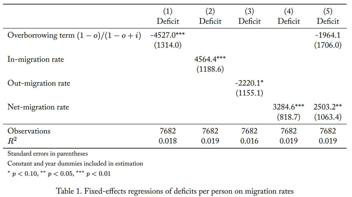
The out-migration rate is negatively correlated with deficits. If causal, this would work against the theory. However, the quantitative model will also give a negative coefficient, and the reason is twofold. First, a negative productivity shock increases out-migration while simultaneously increasing borrowing (for consumption smoothing purposes), which generates positive comovement between out-migration rates and deficits. Second, the overborrowing externality, as reflected in $\frac{1−o}{1−o+i}$ , is far less influenced by out-migration than in-migration, which should make it harder to detect. For example, since $i$ is around 6% in the data, a 10 percentage point increase in the out-migration rate (say from 0 to 0.1) makes the overborrowing term go from around 0.943 to 0.938. In contrast, if $o$ is 6% and i increases from 0 to 10%, the overborrowing term should go from 1 to 0.904. Higher net migration rates also should cause increased borrowing since the effective discount factor can be written $(1 - o)/(1 + net)$ where net is the net migration rate, and this is borne out in the fixed-effects regressions.

In the final specification, we include net migration rates alongside the overborrowing term. This specification is designed to control for effects that may increase deficits not due to overborrowing but rather due to financing of large capital projects, for example. In this specification, the overborrowing term is still negatively correlated with deficits but not at standard confidence levels. While these regressions should not be interpreted causally, they are consistent with the model’s theoretical predictions and indicate a connection between borrowing and migration. Later, we will use these regression results in validating our calibrated model.

Borrowing limits

One of the model’s predictions is that a supra-local planner would generally like to restrict local government borrowing, and that this constraint would generally be binding.⁸ In fact, many states do have statutory limits on how much cities can borrow. To show the variety both in sizes and types of limits, we report in Table 2 borrowing limits for nine states. The table reveals states have implemented a variety of rules. E.g., California (CA) limits are tied to spending or revenue that year. In contrast, most of the states restrict debt based on a percentage of property valuations, but the percentages can differ substantially from as little as 0.2% (IL) to 10% (NY ). Almost all the states have known exceptions, and these usually include debt related to education and or water supplies or voter-approved debt. Qualitatively, the rules in CA and the spending-based exceptions in other states could produce an incentive to have big budgets in order to borrow more, and the quantitative model will allow for this feature of the law.

Are these constraints binding? Here we are limited because our main dataset does not have data on taxable property valuations, and many states use this information in their borrowing limit formulation. However, California uses expenditures to constrain debt, and so we can tell how close cities are to their limit as displayed in the top panel of Figure 1. The graph reveals that many cities—including very large ones—are

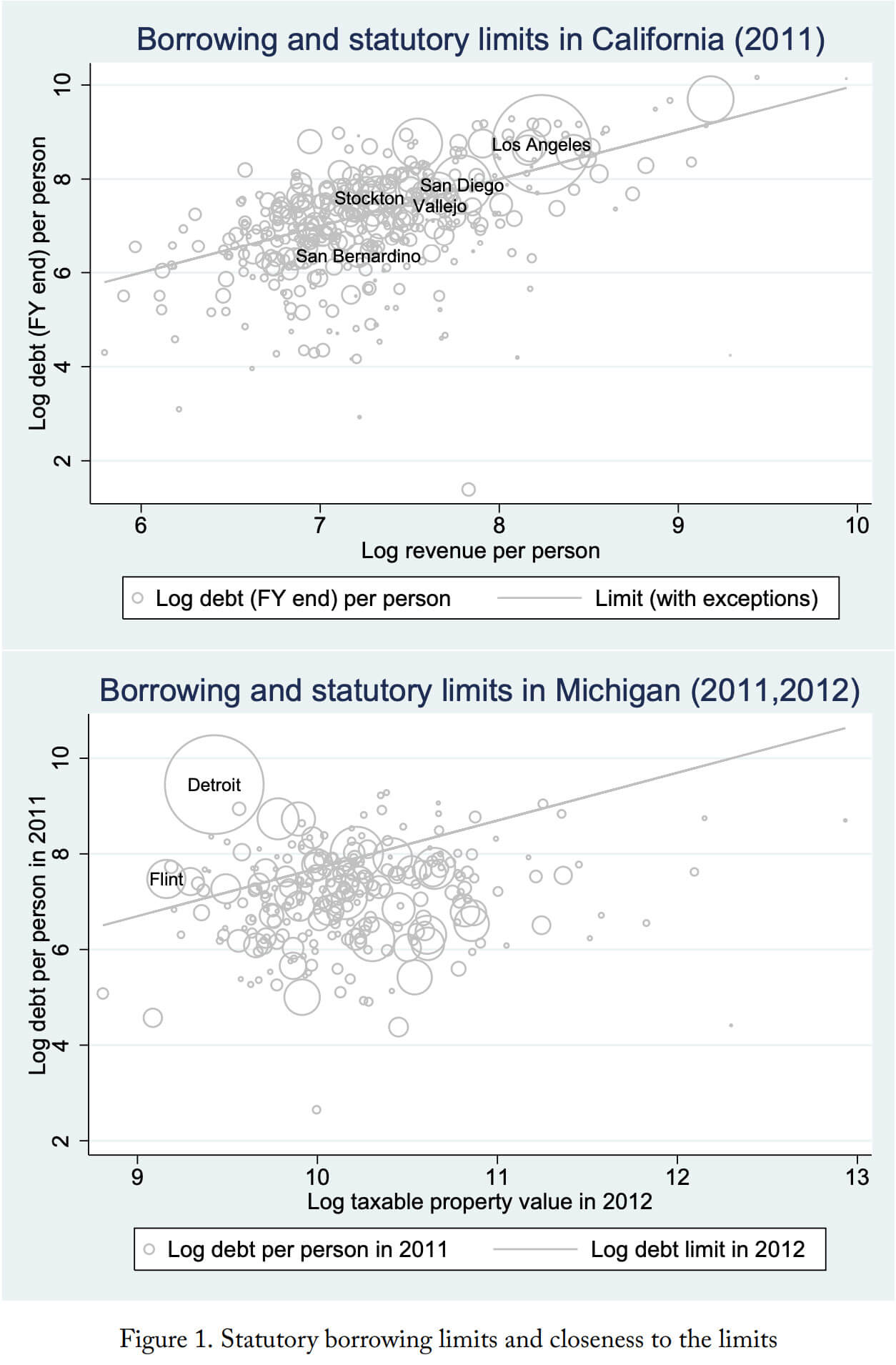
borrowing beyond the revenue per person limit (which could reflect spending on special projects or borrowing authorized by referendum). Additionally, we were able to find taxable valuation data for Michigan (from Kleine and Schulz, 2017), and the bottom panel of Figure 1 displays how close MI cities are to their limits. Again, many cities are at, near, or above the limit, including Detroit and Flint. Even the wealthiest cities (as measured by property values) are borrowing. In summary, it seems cities regularly borrow, and many of them borrow as much as they legally can. This evidence suggests the borrowing limits are binding, consistent with the model prediction that cities are overborrowing and that states are optimally restricting them. Additionally, the quantitative model—where we know overborrowing does occur and can tell explicitly whether the limits are binding—will produce similar patterns and generate a positive (though small) welfare gain from having borrowing limits.

A case study of default and financial distress

To uncover some stylized facts on municipal defaults and financial distress, we turn to a case study of local governments. Our sample is Detroit (MI), Flint (MI), Harrisburg (PA), San Bernardino (CA), Stockton (CA), Vallejo (CA), Chicago (IL), and Hartford (CT), cities that have defaulted or been reported as having financial difficulties in the last few years. (News coverage on these and other cities is listed in Appendix A.)

As emphasized in the introduction, the population growth data shown in the top left panel of Figure 2 reveal heterogeneous paths to default or, more generally, fiscal stress. San Bernardino, Stockton, and Vallejo all experience unusually large population growth leading up to default. Detroit and Flint, and to a lesser extent Chicago, Hartford, and Harrisburg, experience the opposite. Similarly, the top right panel reveals that cities encounter fiscal stress during periods of adverse productivity shocks (Detroit, Flint, Stockton, San Bernardino) or after unusually large productivity gains (Chicago, Vallejo, Hartford). From the lens of standard default models, the latter observation is surprising; but we will show our model can generate defaults after productivity and population booms (as well as busts).

The middle left panel in Figure 2 displays the dynamics of debt in 2012 dollars per person since the mid-1980s. One can see that financially struggling cities tend to have debt far above average. For example, while the average city owed less than $1,000 in 2011, Chicago and Detroit owed about $8,000 and $12,000, respectively. In some cases, financial maneuvering has been used to underplay the amount of debt: Harrisburg’s massive debt in the early 1990s plummeted due to a sale of its incinerator project to a separate government entity (Murphy, 2013).⁹ While the average debt position of all cities looks flat because it is so much smaller than the case study cities’ average, it has increased by 56% since the 1980s, going from $469 per person to $732.

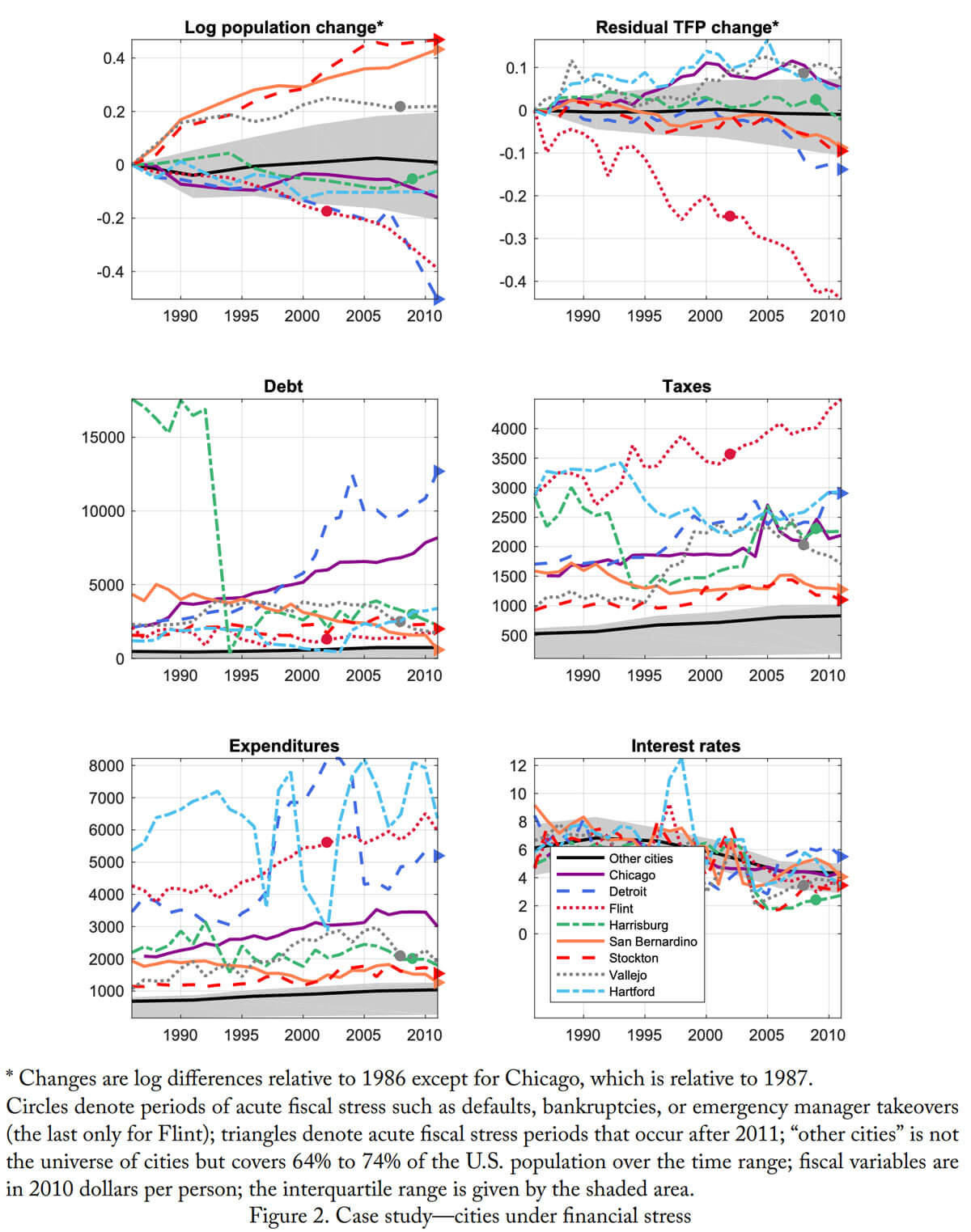
Regarding inlays and outlays (the middle right panel and lower left panel, respectively), we observe that defaulters’ expenditures tend to outstrip their tax revenues, but not always. Furthermore, defaulters have large expenditures per person. In contrast, typical cities seem to run close to balanced budgets, which is consistent with the comparatively low average debt per person. Hartford’s large tax revenue shortfall (with expenditures often around $6,000 and with tax revenue closer to $2,500) has been offset with large cash infusions by the state (Rojas and Walsh, 2017). While Connecticut’s support for Hartford has been exceptional, we will analyze the consequences of this bailout-like behavior in our ”Model predictions and counterfactuals” section.¹⁰

The data reveal a secular decline in interest rates over the past decades and show the financial crisis pushed up the borrowing costs of defaulters in our sample.¹¹ (The data for “other cities” is plotted only in years ending in two or seven, which is when the coverage is almost universal. Consequently, the high frequency variation is missed; see Appendix A.2 for details.) This run up in interest rates likely contributed to the wave of defaults at the end of our sample. Furthermore, the recent increase in the federal fund rates raises the question of whether increased borrowing costs will have significant deleterious effects on city finances. We will also investigate this in our ”Model predictions and counterfactuals section.”
In summary, our case studies uncover the existence of multiple paths to default. These paths are quite heterogeneous with defaults happening during booms and busts. As we will show, the model we will propose is rich enough to capture these heterogeneous default episodes.

Default rates, trends, and institutional details

We close this section by discussing overall default rates and trends, as well as a few relevant institutional details. According to Moody’s (2012), there have been 73 municipal bond defaults (of bonds rated by Moody’s) between 1970 and 2011. This figure translates into a default rate of roughly one municipal default every 4.3 years. These very low default rates imply that municipal bonds generally carry low interest rates, as was seen in Figure 2.

However, this low default rate belies the precarious nature of city finances. For instance, as happened in Flint, cities can come under state management and thereby lose control of their finances. In fact, Kleine and Schulz (2017) report that Michigan in and just before 2017 had 11 cities (4%), one township, and one county under state oversight due to a financial emergency (p. 9).

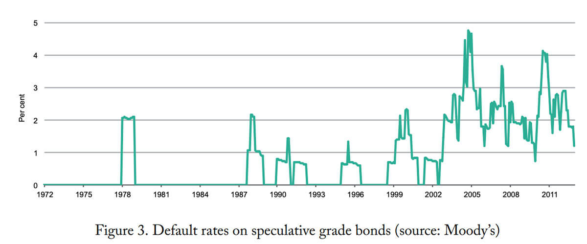
Additionally, the last decade has seen a substantial increase in default rates. Figure 3 shows the default rates for speculative-grade municipal bonds over the past 40 years, and these rates have doubled since the onset of the Great Recession (going from 1% during 1991–2007 to 2% during 2008–2012). These results show that while overall default rates are low, fiscal stress is substantial and potentially growing.

Before moving to the quantitative model, it is important to discuss how we will measure and model debt. There are essentially two issues. The first issue is whether debt should be measured as gross or net of assets. Because municipal bankruptcy (i.e., Chapter 9 bankruptcy) allows municipalities to discharge their debt while keeping essentially all their assets (in contrast to consumer and firm bankruptcy under Chapter 7), we will focus on gross debt (not debt net of assets) in the calibration and treat bankruptcy as a complete discharge of debt.¹²

The second issue is how pension obligations should be treated. In a series of works (Novy-Marx and Rauh, 2009, 2011; Rauh, 2017), Rauh and Novy-Marx have argued that, while officially pensions may be fully funded, they are in fact significantly underfunded when using the appropriate discount rates.¹³ In our benchmark, we treat pensions as fully funded because properly modeling pensions requires three substantial deviations from our already complicated, and novel, model: First, an overlapping generations structure (to have a role for pensions); second, adding pension obligations as a state variable (since the obligations are not dischargeable); and, third, having rate-of-return risk (to evaluate reforms requiring the use of risk-free rather than risky discount rates). However, in Appendix C, as a robustness check we recalibrate the model so that the equilibrium amount of nonpension, defaultable debt is larger by the amount of underfunded obligations reported in Rauh (2017). While we find the differences are very small, more research is needed to properly assess the role of pensions in local finances.

The quantitative model

We first provide an overview of the model and its timing. Then, we describe the household, firm, and government problems. Finally, we define equilibrium.

Overview and timing

We model municipalities in the U.S. as a unit measure of islands. Each island consists of a continuum of households (whose measure in the aggregate is one), a local government, and a neoclassical firm. The government is a sovereign entity that issues debt, taxes its residents, and provides government services. Households consume, work, and crucially decide whether to stay on the island or migrate to another one. Finally, there is a financial intermediary who buys portfolios of municipal debt as well as a risk-free bond.

The timing of the model is as follows. At the beginning of the period, all shocks are realized. Upon observing them, households make migration decisions. After migration occurs, the government chooses its policies, including debt issuance.¹⁴ Finally, households make consumption and labor decisions simultaneously with firms while taking prices and government policies as given.

Households

Define the state vector of a generic island as x := ( $b, n, z, f, w$ ), where $b$ is assets per person measured before migration, $n$ is the population before migration, $z$ is the island’s productivity, $f \in {0, 1}$ indicates whether the government is in a state of default, and $ω$ is a fixed island type we will think of as weather. Including “weather” allows the model to match the variance of population across cities without producing a counterfactually large correlation between productivity and in-migration. We assume $z$ follows a finite-state Markov chain.

Households, knowing x, decide whether to stay $m = 0$ or move $m = 1$ . If they stay, they expect to receive lifetime utility $S(x)$ (specified below). If they move, they are assigned to another island, receive J in expected lifetime utility, and pay an idiosyncratic utility cost $\phi \sim F(\phi|z)$ . The dependence of $\phi$ on $z$ allows us to capture, in a reduced form way, the notion that high-income workers are more mobile than low-income ones; however, the estimated dependence of $F$ on $z$ turns out to be very small. Their problem is

(7) $\begin{equation*} \begin{gathered} V (\phi, x) = max_{m \in \left\{0,1\right\}} (1 − m)S(x) + m(J − \phi). \end{gathered} \end{equation*}$

The moving decision follows a reservation strategy R(x) with $m = 1$ when $\phi < R(x)$ .

The utility conditional on staying is

(8) $\begin{equation*} \begin{gathered} S(x) = max_{c\ge 0,h\ge 0} u(c, g(x), h, ω) + \beta E_{\phi^{\prime},x^{\prime}|x} V (\phi^{\prime} , x^{\prime} )\\ s.t. c + r(x)h = w(x) + \pi(x) − T(x) \end{gathered} \end{equation*}$

where $w(x)$ is the island’s wage; $\pi (x)$ is the per person profit from the island’s firm; $g(x)$ is government services; $T(x)$ are lump-sum taxes (which we will show is virtually equivalent to using property taxes); and h is a housing good, owned by the firm and rented to households at price $r(x)$ . The expectation term $E_{\phi^{\prime} ,x ′|x}$ embeds household beliefs about the local government’s policies. We assume u is continuously differentiable, strictly concave, strictly increasing, and satisfies the Inada conditions in its first three arguments.

If a household decides to move, they migrate to island x at rate $i(x)$ and must stay there for at least one period. We assume that this rate is given by

(9) $\begin{equation*} \begin{gathered} i(x) = \int nF(R(x)|z)d \mu (x) ) \frac{exp(\lambda S(x))} {\int exp(\lambda S(x))d \mu (x)} \end{gathered} \end{equation*}$

where $\mu$ is the invariant distribution of islands.¹⁵ By construction, the measure of households leaving equals the measure entering in aggregate, $\int i(x)d\mu (x) = \int nF(R(x))d \mu (x)$ . If $\lambda = 0$ , households are uniformly assigned to each island (“random search”). As λ → ∞, the city with the largest S(x) receives all the inflows (“directed search”). Note that these inflows are what would arise from using Type 1 extreme value shocks (as in Kennan and Walker, 2011, and many others) were there a finite number of islands.¹⁶ Given these inflows, the expected value of moving in equilibrium is

(10) $\begin{equation*} J=\int S(\mathbf{x}) \frac{i(\mathbf{x})}{\int i(\mathbf{x}) d \mu(\mathbf{x})} d \mu(\mathbf{x}) \end{equation*}$

and the law of motion for population is

(11) $\begin{equation*} \dot{n}(\mathbf{x})=n(1-F(R(\mathbf{x}) \mid z))+i(\mathbf{x}) \end{equation*}$

where n˙ denotes the population after migration has taken place.

Firms

Each island has a firm that operates a linear production technology zL and owns the island’s housing stock $\overline{H}$ . Alternatively, $\overline{H}$ may be thought of as the island’s land. We assume $\overline{H}$ is in fixed supply and homogeneous across islands to prevent adding an extra state variable, but our inclusion of weather ω will capture some of this fixed heterogeneity across islands. Firms solve

(12) $\begin{equation*} \dot{n}(\mathbf{x}) \pi(\mathbf{x})=\max _{L, H \leq \bar{H}}(1-\kappa(\mathbf{x})) z L-w(\mathbf{x}) L+r(\mathbf{x}) H \end{equation*}$

taking w and r competitively, and the solution of this problem gives labor demand, L d (and the housing supply, H = $\overline{H}$ ). The term $K(x) = K \left\{d(x), f \right\}$ is a pecuniary cost of default. Since n˙(x) denotes the number of households remaining after migration and each household inelastically supplies one unit of labor, labor market clearing requires

(13) $\begin{equation*} L^d(\mathrm{x})=\dot{n}(\mathbf{x}) \end{equation*}$

It is worth making a few observations about the firm problem. First, in equilibrium, per person profits π equal rH/n˙ . Consequently, by making local residents the firm shareholders, we are effectively assuming each gets the rent associated with owning an equal share of the housing/land stock. Second, if there were property taxes, say via τ r(x)H for τ $\in$ [0, 1], the taxes would reduce these rents by τ rH/n˙ in the same way that the lump-sum tax T in (8) does. For this reason, we loosely interpret the lump-sum tax T as a property tax. Last, we have assumed there are no agglomeration or congestion effects in the production function (or that they are both present and cancel).¹⁷ Their absence could result in the model under- or over-predicting the relationship between population and productivity. However, the model generates a signficant positive correlation between city density and productivity like that found in the data (Glaeser, 2010). Also, the model has congestion externalities in the form of reduced housing per person and agglomeration effects in that local governments provide a partly nonrival service, as will be discussed shortly.

Local governments

Each local government decides the level of services g ≥ 0 it wishes to provide. These services are potentially nonrival in that, to provide g services to each of the n˙ households, the government must only invest n˙ 1−η g units of the consumption good where η ∈ [0, 1] is a parameter. The government pays for these services using tax revenue Tn˙ or, potentially, debt issuance. The default flag f (which is a component of x) indicates the city’s standing with creditors. If f = 0, then the city is in good standing with its creditors and can borrow and default. If f = 1, it is in bad standing and cannot borrow (and has no debt). In the case of default or bad standing, firm output drops by κ and the government returns to good standing f ′ = 0 and no debt b ′ = 0 with probability χ. A government with f = 0 that repays its debt −bn chooses a new level of debt per person −b′ , implying a total obligation next period of −b ′n˙ . The discount price it receives on this pledge is q(b′, n, z, ω ˙ ), which depends on the debt level, population after migration n˙ (which equals the next period’s population before migration n ′ ), productivity, and weather, as all of these potentially influence repayment rates.¹⁸

In keeping with the statutory borrowing limits discussed in our ”Data and institutions” section, we impose a borrowing limit b ′ ≥ b(z, n, g ˙ ). For the quantitative work, we further assume that

(14) $\begin{equation*} -b^{\prime} \leq g \dot{n}^{-\eta} \delta \end{equation*}$

where δ ∈ R + controls how tight the limit is. Hence, we require total debt issued in a period −b ′n˙ to be less than a fraction δ of total expenditures gn˙ 1−η . Note that this limit is qualitatively closer to the standard limits in CA than the other states. However, the exemptions in many states allow for spending on projects, which this form permits. Given the large variation in laws across states, we will choose δ to match observed debt levels rather than trying to choose it based on statutory law. However, the estimated value will be not far from California’s statutory limit of δ = 1.

To define the government’s problem, we need to specify how the economy will respond to deviations in government policies. To this end, we assume r and w adjust dynamically in response to the government policies (d, g, b′ , and T) clearing the labor and housing markets and that households and firms optimize given those prices and implied profits. Formally, we assume that c, h, r, w, π, Ld always solve the following equations

(15) $\begin{equation*} \begin{gathered} u_c r=u_h \\ \underbrace{c+r h=w+\pi-T}_{\text {Household optimization }} \end{gathered} \underbrace{\begin{array}{c} w=(1-\bar{\kappa} \hat{d}) z \\ \dot{n} \pi=(1-\bar{\kappa} \hat{d}) z L^d-w L^d+r \bar{H} \end{array}}_{\text {Firm optimization }}, \text { and } \underbrace{\begin{array}{c} \dot{n}=L^d, \\ \dot{n} h=\bar{H} \end{array}}_{\text {Market clearing }}, \end{equation*}$

where ˆd := max{d, f}. Letting U denote the indirect flow utility associated with g, T, and d, it is easy to show

(16) $\begin{equation*} U(g, T, \hat{d}, \dot{n}, z, \omega)=u((1-\bar{\kappa} \hat{d}) z-T, g, \bar{H} / \dot{n}, \omega) \end{equation*}$

Now we can state the government’s problem as

(17) $\begin{equation*} \tilde{S}(\mathrm{x})= \begin{cases}\max _{d \in\{0,1\}}(1-d) S^N(\dot{b}(\mathrm{x}), \dot{n}(\mathrm{x}), z, \omega)+d S^D(\dot{b}(\mathrm{x}), \dot{n}(\mathrm{x}), z, \omega) & \text { if } f=0 \\ S^D(\dot{b}(\mathbf{x}), \dot{n}(\mathbf{x}), z, \omega) & \text { if } f=1\end{cases} \end{equation*}$

where ˙b(x) := bn/ ˙n(x) gives assets per person after migration and

(18) $\begin{equation*} \begin{gathered} \tilde{S}^N(\dot{b}, \dot{n}, z, \omega)=\max _{g \geq 0, T \leq z, b^{\prime} \in \mathrm{B}} U(g, T, 0, \dot{n}, z, \omega)+\beta \mathbb{E}_{\phi^{\prime}, z^{\prime} \mid z} \tilde{V}\left(\phi^{\prime}, b^{\prime}, \dot{n}, z^{\prime}, 0, \omega\right) \\ \text { s.t. } g \dot{n}^{1-\eta}+q\left(b^{\prime}, \dot{n}, z, \omega\right) b^{\prime} \dot{n}=T \dot{n}+\dot{b} \dot{n} \\ b^{\prime} \geq \underline{b}(z, \dot{n}, g) \end{gathered} \end{equation*}$

and

(19) $\begin{equation*} \begin{gathered} \tilde{S}^D(\dot{b}, \dot{n}, z, \omega)=\max _{g \geq 0, T \leq(1-\bar{\kappa}) z} U(g, T, 1, \dot{n}, z, \omega)+\beta \mathbb{E}_{\phi^{\prime}, z^{\prime} \mid z}\left(\begin{array}{r} \chi \tilde{V}\left(\phi^{\prime}, 0, \dot{n}, z^{\prime}, 0, \omega\right) \\ +(1-\chi) \tilde{V}\left(\phi^{\prime}, \dot{b}, \dot{n}, z^{\prime}, 1, \omega\right) \end{array}\right) \\ \text { s.t. } g \dot{n}^{1-\eta}=T \dot{n} \end{gathered} \end{equation*}$

with V˜ (ϕ, x) = max{S˜(x), J − ϕ}. (Note that in (18) we used the identity bn = ˙bn˙ .) For the quantitative work and most of the theoretical results, we restrict the bond choice b ′ to be in a finite set B that includes 0. For the derivation of the Euler equation, however, we treat B as an interval [b, ∞) with b < 0.

Financial intermediaries

Following Chatterjee, Corbae, Nakajima, and Ríos-Rull (2007), we posit a competitive financial intermediary who purchases measures of contracts. To write the intermediary’s problem, we think of governments and the intermediary as choosing contracts indexed by (b ′ , n′ , z, ω)—note n ′ = ˙n. From the government’s perspective, a contract costs Q(b ′ , n′ , z, ω) := q(b ′ , n′ , z, ω)b ′n ′ in the current period, yields b ′n ′ if the city does not default, and yields zero otherwise. Because the intermediary purchases a measure of contracts, a law of large numbers gives a certain yield $\Sigma_{z^{\prime}} P(z^{\prime} |z)(1 − d(b^{\prime} , n^{\prime} , z^{\prime} , w))b^{\prime} n^{\prime}$ . The intermediary behaves competitively, taking Q and d as given.

The intermediary chooses a measure M′ over contracts to maximize the net present value of dividends D discounted at rate $\overline{q}.$ His problem is

(20) $\begin{equation*} \begin{aligned} & W(B, M)=\max _{D, B^{\prime}, M^{\prime}} D+\bar{q} W\left(B^{\prime}, M^{\prime}\right) \\ & \text { s.t. } D+\bar{q} B^{\prime}+\int Q\left(b^{\prime}, n^{\prime}, z, \omega\right) d M^{\prime}\left(b^{\prime}, n^{\prime}, z, \omega\right)=B+\int \sum_\gamma \mathbb{P}\left(z \mid z_{-1}\right)(1-d(b, n, z, \omega))(b n) d M\left(b, n, z_{-1}, \omega\right) \text {, } \\ & \end{aligned} \end{equation*}$

with a no-Ponzi condition.

In equilibrium, we require that (1) the intermediary issues zero dividends each period (D = 0); (2) the intermediary has zero wealth (W = 0); (3) contract markets clear; and (4) the risk-free bond market clears. We assume the risk-free bond is in net supply B, and so bond market clearing requires B′ = B = B. We further assume each contract is in zero net supply, which means the intermediary must be the counterparty to every contract purchased by cities. Formally, contract markets clear if

(21) $\begin{equation*} M^{\prime}(\mathcal{B}, \mathcal{N}, z, \omega)=-\int \mathbf{1}_{\left[b^{\prime}(b, n, z, 0, \omega) \in \mathcal{B}, \dot{n}(b, n, z, 0, \omega) \in \mathcal{N}\right]}(1-d(b, n, z, \omega)) \mu(d b, d n, z, 0, \omega) \end{equation*}$

for all z, ω and all B × N in a product Borel σ-algebra. Our assumption that the economy is closed is particularly appropriate for municipal bonds, as approximately 97% of them are held domestically (Cohen and Eappen, 2015). An attractive implication of the zero-dividend condition is that we do not need to specify who owns the intermediary.

Equilibrium

A steady-state recursive competitive equilibrium is value functions S, V, S, ˜ V˜ ; an expected value of moving J; household policies c, h, m; government policies g, T, b′ , d; prices and profit q, q, w, r, π ¯ ; labor demand L d ; the intermediary policies and value function D, M′ , B′ , W; an intermediary state M; a law of motion for population n˙ ; and a distribution of islands µ, such that (1) household policies c, h and migration decisions are optimal taking V , S, J, prices and government policies as given; (2) government policies g, T, b′ , d are optimal taking V˜ , S˜, J, the population law of motion n˙(x), and prices q as given; (3) firms optimally choose L d (x) taking w(x), r(x) as given and optimal per person profits are π(x); (4) the intermediary policies D, M′ , B′ are optimal given W, q, q, ¯ and d; (5) beliefs are consistent: S(x) = S˜(x) and V (ϕ, x) = V˜ (ϕ, x); (6) the distribution of islands µ is invariant; (7) the intermediary’s portfolio is time-invariant, M = M′ (B, M); (8) J and n˙ are consistent with µ and household and government policies; (9) the intermediary makes zero profits, D(B, M) = 0 and W(B, M) = 0; and (10) markets clear.

Centralization and the Euler equation

To characterize equilibrium, we first simplify the equilibrium conditions by providing sufficient conditions for the intermediary’s problem, bond-market clearing, and contract market-clearing to be satisfied. We then show how the government and household problems may be centralized into a single problem. Last, we derive the Euler equation.

Proposition 6. If prices satisfy

(22) $\begin{equation*} q\left(b^{\prime}, n^{\prime}, z, \omega\right)=\bar{q} \mathbb{E}_{z^{\prime} \mid z}\left(1-d\left(b^{\prime}, n^{\prime}, z^{\prime}, \omega\right)\right) \end{equation*}$

and if

(23) $\begin{equation*} \bar{B}=\int(1-d(b, n, z, \omega)) b n \mu(d b, d n, d z, 0, d \omega) \end{equation*}$

then there exist prices and an optimal policy M′ , with M′ invariant, such that contract markets and the risk-free bond market clear and zero profits obtain (provided the other equilibrium conditions are met).

Note that if there is no default, this simply says B = R bndµ, which means in equilibrium the intermediary holds a portfolio of city assets / debt (R bndµ) that corresponds to aggregate debt demand (−B).

Proposition 7 shows the government, household, and firm problem may be centralized into a single problem, which we use as the basis for computation.

Proposition 7. Suppose Sˆ satisfies

(24) $\begin{equation*} \hat{S}(\mathrm{x})= \begin{cases}\max _{d \in\{0,1\}}(1-d) \hat{S}^N(\dot{b}(\mathrm{x}), \dot{n}(\mathrm{x}), z, \omega)+d \hat{S}^D(\dot{b}(\mathrm{x}), \dot{n}(\mathrm{x}), z, \omega) & \text { if } f=0 \\ \hat{S}^D(\dot{b}(\mathrm{x}), \dot{n}(\mathrm{x}), z, \omega) & \text { if } f=1\end{cases} \end{equation*}$

where

(25) $\begin{equation*} \begin{gathered} \hat{S}^N(\dot{b}, \dot{n}, z, \omega)=\max _{c>0, g \geq 0, b^{\prime} \in \mathrm{B}} u(c, g, \bar{H} / \dot{n}, \omega)+\beta \mathbb{E}_{\phi^{\prime}, z^{\prime} \mid z} \max \left\{\hat{S}\left(b^{\prime}, \dot{n}, z^{\prime}, 0, \omega\right), J-\phi^{\prime}\right\} \\ \text { s.t. } \dot{n} c+\dot{n}^{1-\eta} g+q\left(b^{\prime}, \dot{n}, z, \omega\right) b^{\prime} \dot{n}=z \dot{n}+\dot{b} \dot{n} \\ b^{\prime} \geq \underline{b}(z, \dot{n}, g) \end{gathered} \end{equation*}$

and

(26) $\begin{equation*} \begin{gathered} \hat{S}^D(\dot{b}, \dot{n}, z, \omega)=\max _{c>0, g \geq 0} u(c, g, \bar{H} / \dot{n}, \omega)+\beta \mathbb{E}_{\phi^{\prime}, z^{\prime} \mid z}\left(\begin{array}{r} \chi \max \left\{\hat{S}\left(0, \dot{n}, z^{\prime}, 0, \omega\right), J-\phi^{\prime}\right\} \\ +(1-\chi) \max \left\{\hat{S}\left(\dot{b}, \dot{n}, z^{\prime}, 1, \omega\right), J-\phi^{\prime}\right\} \end{array}\right) \\ \text { s.t. } \dot{n} c+\dot{n}^{1-\eta} g=(1-\bar{\kappa}) z \dot{n} \end{gathered} \end{equation*}$

with associated optimal policies c(x), g(x), d(x), b′ (x) (with d and b ′ arbitrary for f = 1). Then (1) Sˆ is a solution to the household problem and c, l are optimal policies; (2) Sˆ is a solution to the government problem and g, d, b′ are optimal policies; and (3) there exists prices r, w such that labor and housing markets clear and firms optimize.

In what follows, we will use S, SN , SD in place of S, ˆ SˆN , SˆD, respectively

Proposition 8 characterizes the government Euler equation:

Proposition 8. Consider the S N problem in (25) at some state ( ˙b, n′ , z). Suppose that at the optimal choices, the borrowing constraint is not binding and that locally about b ′ repaying is strictly preferred. If in addition S N ˙b (b ′ n ′ n′′ , n ′′, z′ , ω), S N n˙ (b ′ n ′ n′′ , n ′′, z′ , ω), and n˙ b(b ′ , n′ , z′ , 0, ω) exist locally for n ′′ := ˙n(b ′ , n′ , z′ , 0, ω) about b ′ , then the Euler equation satisfies

(27) $\begin{equation*} u_c \bar{q}=\beta \mathbb{E}_{z^{\prime} \mid z}\left[u_c\left(\frac{1-o^{\prime}}{1+i^{\prime}-o^{\prime}}\right)\left(1-\frac{b^{\prime}}{n^{\prime \prime}} \dot{n}_b\right)+\left(1-o^{\prime}\right) S_{\dot{n}}^N\left(b^{\prime} \frac{n^{\prime}}{n^{\prime \prime}}, n^{\prime \prime}, z^{\prime}, \omega\right) \dot{n}_b\right] \end{equation*}$

where o ′ is the outflow rate F(R(b ′ , n′ , z′ , 0)|z ′ ) and i ′ = i(b ′ , n′ , z′ , 0)/n ′ is the inflow rate next period.

Relative to the two-period model Euler equation in (2), there is an additional term connected to S N n˙ . In the two-period model, the level of population only effects utility through its effect on debt per person. Here, there are additional effects through reduced housing per person (H/n˙) and partially nonrival government services (if η > 0).

One result we would like to have is a proof of equilibrium uniqueness. Unfortunately, we have not been able to show uniqueness even in the general version of the two-period model. This is potentially worrisome in that, given the link between migration and borrowing we demonstrated, expectations of how many people are moving might feed into debt accumulation decisions and justify those expectations. However, we investigate uniqueness quantitatively by using 100 randomly drawn initial guesses for the equilibrium objects. Each guess converged to the same equilibrium values, and so at least computationally there is no evidence of indeterminacy at the calibrated values. See Appendix D.6 for more details.

Calibration and estimation

In this section, we show that the model can reproduce a large number of key empirical moments, targeted and untargeted. The data, including definitions, construction, and cleaning of key variables, are described in Appendix A. We take a model period to be a year.

Productivity

As productivity (TFP) plays a vital role in the model, it is necessary to have a process that accurately captures location-specific productivity dynamics. To this end, we begin by constructing a TFP series in the data using the County Business Patterns (CBP), which is an annual panel dataset published by the Census covering the universe of counties (not cities, unfortunately) dating back to 1986.¹⁹ For our TFP measure, we use real annual payrolls per employee.

Let TFP for a county-year pair be denoted zit. We specify

(28) $\begin{equation*} \log z_{i t}=\varsigma_i+\varpi_t+\tilde{z}_{i t} \end{equation*}$

and obtain the residual z˜it using a fixed-effects regression. To discretize the fixed effects ςi , we nonparametrically break the estimates into bins corresponding to to 0–10%, 10–50%, 50–90%, 90–99%, and 99–100%. The estimated fixed effects averaged within these bins are −0.34, −0.13, 0.09, 0.37, and 0.65, respectively. We discard the time effects ϖt as we will only consider steady states.

For the residual TFP z˜it, we use an AR(2) specification, which allows more persistent movements in TFP that better capture decade-long persistent movements in productivity such as what occurred in Detroit and Flint (see Figure 2). Restricting the sample to cities of at least one million residents, the estimated first and second AR coefficients are 0.73 (0.02) and 0.23 (0.03), respectively, with an innovation variance 0.001 (2 × 10−5 ).20 We describe our discretization process in the appendix.

Preferences and moving costs

We set β = 0.96 and assume the flow utility exhibits constant relative risk aversion over a Cobb-Douglas aggregate of consumption, government services, and housing plus a taste shifter for weather:

(29) $\begin{equation*} u(c, g, h, \omega)=\frac{\left(c^{1-\zeta_g-\zeta_h} g^{\zeta_g} h^{\zeta_h}\right)^{1-\sigma}}{1-\sigma}+\omega \end{equation*}$

As ζg and ζh are relatively small, the constant relative risk aversion over consumption is approximately σ, which we take to be 2. The free parameters ζg and ζh are estimated jointly, strongly controlling the mean level of government expenditures and housing expenditures, respectively. We take the weather term ω—which is fixed over time for any given region but heterogeneous across regions—to be normally distributed with mean zero (a normalization) and standard deviation σω. We discipline σω by matching the standard deviation of log population across cities.

We assume the moving cost is distributed

(30) $\begin{equation*} \phi \mid z \sim\left\{\begin{array}{ll} \underline{\phi} & \text { w.p. } p_{\underline{\phi}} / 2 \\ \operatorname{Logistic}\left(\mu_\phi-\beta_\phi \log z, \varsigma_\phi\right) & \text { w.p. } 1-p_{\underline{\phi}} \\ -\underline{\phi} & \text { w.p. } p_{\underline{\phi}} / 2 \end{array} .\right. \end{equation*}$

Having the ±ϕ shock means that, for a sufficiently large ϕ, every island’s departure rate is in [pϕ/2, 1 − pϕ/2], which ensures some minimal stability in calibrating the model. Having the mean of the logistic distribution be contingent on z is meant to capture the idea that high-productivity individuals have lower moving costs, but the estimated value of βϕ is approximately zero. We set pϕ = 10−4 and take ϕ arbitrarily large giving R V (ϕ, x)dF(ϕ|z), the expected utility of being in an island with state x, equal to

(31) $\begin{equation*} \frac{p_\phi}{2}(J+S(\mathbf{x}))+\left(1-p_\phi\right)\left(S(\mathbf{x})+\varsigma_\phi \log \left(1+e^{\left(S(\mathbf{x})-J-\mu_\phi+\beta_\phi \log (z)\right) / \varsigma_\phi}\right)\right) \end{equation*}$

plus a constant that we offset via a normalization.²⁰

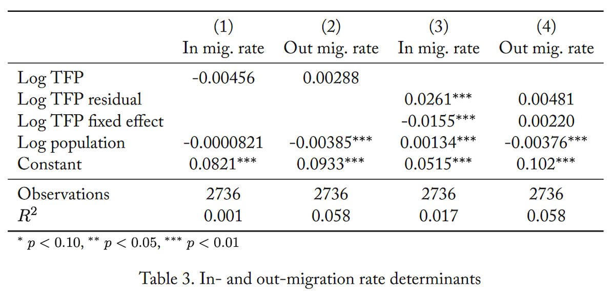
The parameters controlling moving costs µϕ, βϕ, ςϕ and the parameter λ controlling how directed moving is (see (9)) are jointly estimated. We identify the cost parameters using mean departure and arrival rates as well as coefficients from the regressions in Table 3 of productivity and population on outflow rates in the data. βϕ controls how the outflow rate varies with productivity, so we use it to target the regression coefficient for log productivity on outflow rates. ςϕ controls how much the migration decisions vary with fundamentals, so we use the standard deviation of out-migration rates to discipline it. µϕ controls the overall level of outflow rates, so we use the mean departure rate of 6.4% to discipline it. We identify λ by matching the regression coefficient for log TFP fixed effect on log population.

The borrowing limit δ and risk-free bond net supply B jointly determine the overall level of debt in the economy and the equilibrium interest rate associated with q¯. Consequently, we use them to target a mean risk-free interest rate of 4% (the recent average, see Figure 2) and the data’s total debt to GDP ratio of 0.089.22 Since η controls the relative price of government services as population grows, we use the coefficient of a regression of log population on log expenditures (1.113) to discipline it. Finally, we calibrate the default cost κ to match default rates in the data. Since it is difficult to separately identify κ and χ (the probability of returning from autarky), we set χ = 1, which concentrates all default costs in the period of default.

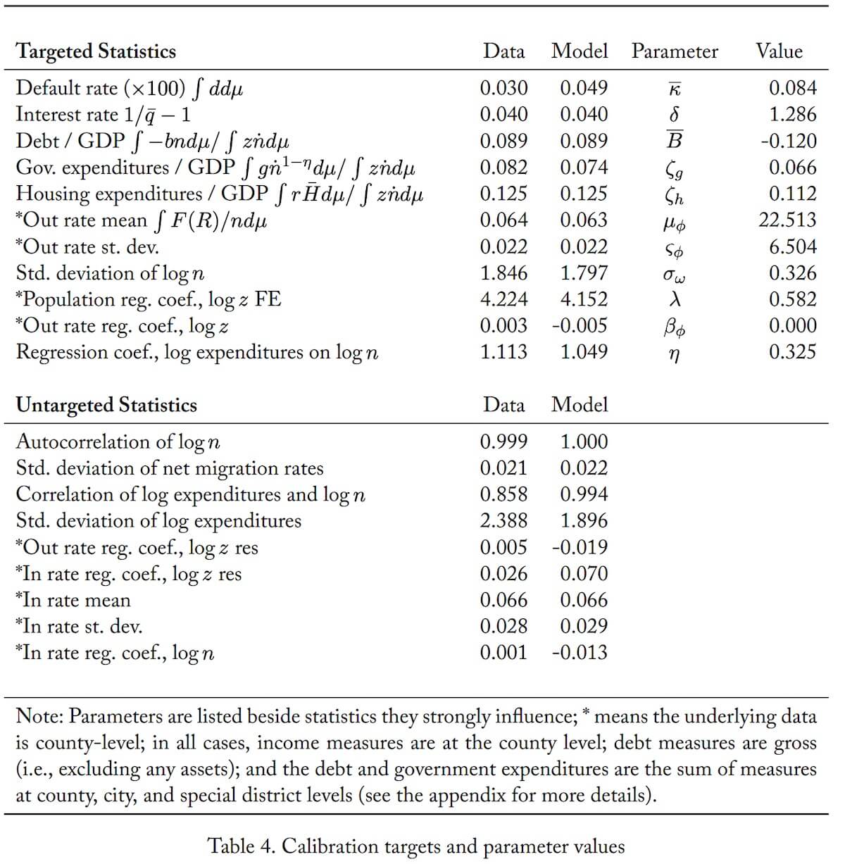
Fit of targeted and untargeted moments

Table 4 reports the targeted and untargeted statistics alongside the jointly calibrated parameter values. The model closely matches all of the targeted statistics. The estimated debt limit, δ, allows cities to borrow up to 128% of their expenditures, which is fairly close to California’s statutory limit of 100% (plus exceptions). The consumption-equivalent flow cost of default, κ, is estimated to be around 3%.²¹ The utility shares ζg and ζh are close to the shares observed in the data. Migration is partially directed with λ > 0. Weather plays a large role, with a rough calculation giving the lifetime consumption equivalent variation of permanently moving from the median weather ω = 0 to 2σω at 67%.²² The importance of weather for utility helps the model match the very low (in fact, negative) correlation between in-migration and productivity and, simultaneously, the large dispersion in population. The large value for µϕ with a correspondingly large ςϕ makes out-migration largely dependent on moving cost shocks rather than fundamentals like productivity. The value for βϕ is nearly zero. Finally, the provision of public goods displays some rivalry with η = 0.33.

The model gets most of the untargeted predictions qualitatively correct while missing on a few statistics. The model recreates the very slow population adjustments seen in the data with log population autocorrelation exceeding the data’s 0.999. It also matches the small correlations between migration rates and productivity and migration rates and population. Last, it reproduces the dispersion in net migration rates and the large dispersion in government expenditures.

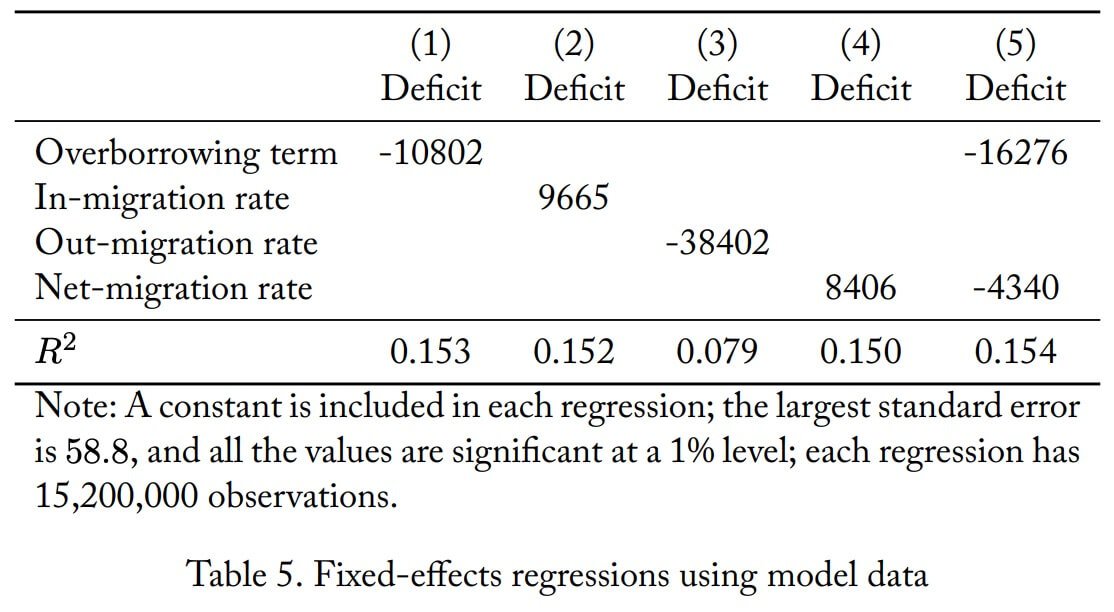
As an additional validation step, we rerun the fixed effects regressions from Table 1 on simulated data from the model. To convert the numeraire to dollars for this example and in the remainder of the paper, we multiply by 50,000, giving average output per person in our benchmark as $68,200. This is between the median and mean household income in 2010 but closer to the median.²³ The results are presented in Table 5, which reveals the model has similar patterns with the overborrowing term (1 − o)/(1 − o + i) and in-migration significantly moving borrowing. One difference is that out-migration, while having the same negative sign as in the data, is much more negative. This reflects an optimal response present in the model that is less dramatic in the data. In particular, when bad productivity causes populations to shrink, the model suggests cities should cut deficits sharply to prevent exploding debt per person, but in the data cities seem not to do this (at least to such an extent). Overall, the magnitudes (except for out-migration) are fairly similar to the data. This feature will reappear in comparing Detroit’s optimal and actual path. The R2 is naturally larger than in the data as there are fewer determinants of spending in the model, but still the regressors explain at most 15% of the variation.

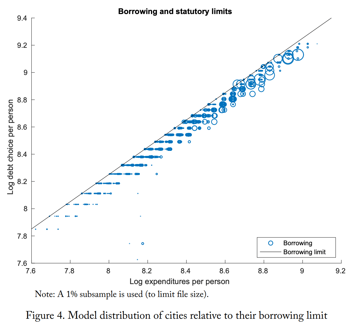
A final validation step is to compare the pattern of cities in relation to the borrowing constraint, which is done in Figure 4. The pattern is remarkably similar to that for California seen in Figure 1. (Note we use a CA-type borrowing limit that ties debt to spending rather than debt to property values like in MI.) Specifically, almost all the cities are close to the statutory borrowing limit, though only a few are exactly at it. As this pattern is nontargeted, it lends additional credence to the model’s other predictions and the counterfactuals that we now analyze.

population loss over the 10 years leading up to default, qualitatively similar to the experience of Flint and Detroit. Facing this shrinking population, the sovereign holds debt per person constant, which requires running a significant primary surplus of almost $200 per year.²⁴ This surplus is financed with cuts to expenditures and taxes. In the few years before default, interest rates do increase, reflecting the increased default risk, but the largest interest rates are still low, not unlike in the data (as can be seen in Figure 2).

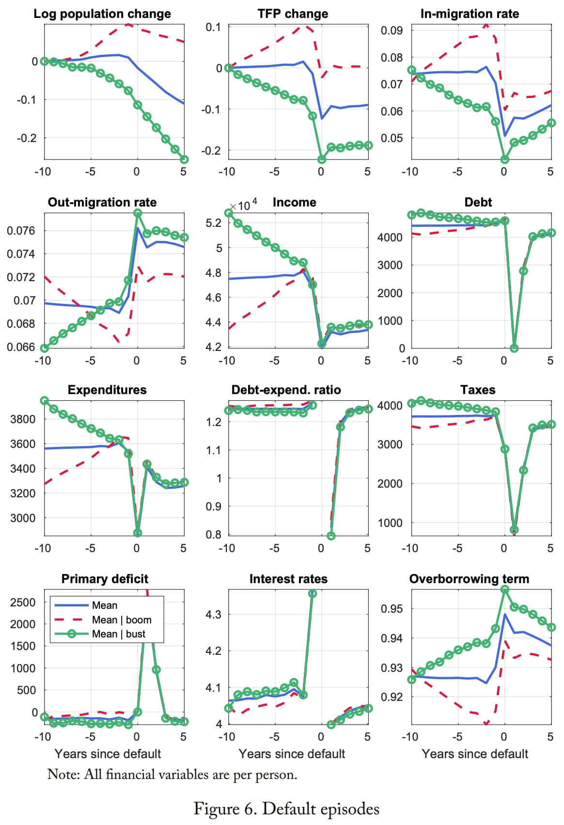
Looking at boom defaults (red dashed lines), the first thing to notice is the model can generate them (which was not clear a priori). The population and productivity growth is strong until just a year before default, like in Vallejo, CA. With the boom, the cities have virtually no primary deficit, which results in growing debt per person as interest payments pile up, and this is despite substantial population growth that all else equal reduces debt per person. The debt growth is paired with a noticeable increase in expenditures and taxes. Interest rates trend upward, showing that the city is taking on increasing (albeit small) amounts of risk. When an unusually large decline in productivity occurs, in-migration plummets and debt per person increases, triggering default. While boom defaults are triggered by a decline in productivity, a necessary ingredient is that the city must be leveraged enough to make default worthwhile. This is where overborrowing plays a crucial role in generating boom defaults: by keeping cities in debt even after long periods of growing productivity, it leaves even high-productivity cities at risk of default.

A striking difference between the boom and bust defaults appears in the incentive to borrow as reflected in the “overborrowing term” (1 − o)/(1 − o + i). In boom defaults, increases in in-migration drive down the overborrowing term, which increases borrowing incentives. The converse is true for bust defaults. Additionally, the magnitudes of the changes are large: recalling that 1 − (1 − o)/(1 − o + i) is the share of debt subsidized (i.e., paid for) by new entrants, in boom (bust) defaults this subsidy increases (decreases) by 2 percentage points. While the debt paths show trends qualitatively consistent with these changes, the dynamics are muted in part because cities are close to their debt limits: the debt-expenditure ratio is close to its limit of δ (1.286) in every year leading up to default.

In answer to the questions of what leads to and triggers default, the model reveals much the same answer as the data: The causes are myriad. Bust defaults lead to shrinking populations and primary surpluses financed by cuts to taxes and larger cuts to expenditures. In contrast, boom defaults are characterized by growing populations, growing debt per person, and growing taxes and expenditures. Boom defaults are possible in the model because of large overborrowing incentives that keep cities leveraged even after a decade of productivity and income growth.

Before moving to the next section, it is important to note one possible concern with our analysis. Specifically, cities drastically—and frictionlessly—lower government expenditures in default. However, since part of government expenditures is capital investment, it may be difficult or costly to reduce expenditures in times of crisis. In Appendix C, we investigate the model’s robustness to this feature by imposing a lower-bound on government services that binds close to and during default. This modification keeps government expenditures and taxes suboptimally high at and around default, resulting in additional population loss during the default event. However, the changes end up being quite small because productivity is the main driver of migration, not deviations in government expenditures.

Disentangling the roles of migration, borrowing limits, credit markets, and general equilibrium effects

The analysis of what drives defaults showed that while defaulters tend to have large debt-expenditure ratios and greater overborrowing incentives than typical cities, the dynamics of debt per person are surprisingly muted. The reason given above was that debt is constrained by the exogenous borrowing limit, which keeps it from from moving much. However, the model has three external forces that restrict borrowing: exogenous borrowing limits, a Laffer curve for borrowing in private credit markets, and the endogenously determined risk-free interest rate. Additionally, the level of in-migration and its elasticity with respect to debt act as internal restraints on borrowing. We now try to assess the role of each of these forces before turning to the counterfactuals.

External restraints on borrowing

To start, we first eliminate the borrowing constraint in partial equilibrium, i.e., holding q¯ fixed at the benchmark. The percent change relative to the benchmark is displayed in the third column (labeled “(∞, ·)”) of Table 6. One can see there is very little change from the benchmark except that the default rate increases somewhat. This is because private credit markets are restraining cities. To show this, we make default infeasible by setting the default cost κ¯ = 1 in addition to having δ = ∞. This eliminates the Laffer curve for debt by turning the borrowing schedule −q(b ′ , n, z, ω ˙ )b ′ , which has a peak, into just −qb¯ ′ , which does not. Those results are displayed in the fifth column, labeled “(∞, 1)”. Now debt per person expands by 65.9%, reaching the maximum debt amount allowed by the computational method ($10,000 per person).²⁵ One interesting feature of these results is that private credit markets restrain borrowing significantly despite small equilibrium default rates. Hence, in our calibration the threat of default, rather than outright losses from default, constrains borrowing.

In fact, our calibration suggests that private credit markets restrain municipal borrowing more than the exogenous borrowing limit. This can be seen in the fourth column, labeled (·, 1), where we have made default costs infinite but kept the borrowing limit at the benchmark value. In this case, debt per person increases by 12.5%. Note that in this case aggregate debt over aggregate expenditures rises from 1.201 to 1.285. Since the benchmark value of δ = 1.286 constrains the debt-expenditure ratio in individual cities to 1.286, this shows that without the Laffer curve from borrowing in private credit markets, virtually every city goes to the borrowing limit in the model.

A final force in the model that restrains borrowing is the general equilibrium response of the risk-free interest rate. In particular, it is sufficient to discuss the most extreme case of (δ, κ¯) = (∞, 1) in the rightmost column of Table 6. In it, we see that while the overborrowing incentives are very large, they can be undone by a strong general equilibrium response that increases the risk-free rate from 4% to 8.8%, thereby keeping debt levels approximately at the benchmark level.²⁶ From these experiments, we conclude that the strong overborrowing incentives seen in the two-period model are present in the quantitative model, but that they are significantly restrained by both exogenous and endogenous (i.e., Laffer curve) credit limits.

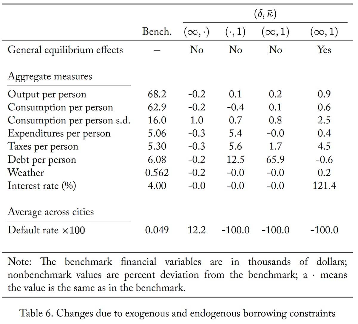
Internal restraints on borrowing

In the two-period model, there were two forces that determined how much the city wanted to overborrow. First was the magnitude of the overborrowing term (1 − o)/(1 − o + i). Second was the elasticity of population with respect to debt accumulation. We change the magnitudes of these forces by increasing and decreasing the mean moving costs µϕ (which primarily affects the first force) and the search directedness parameter λ (which substantially affects both) holding the risk-free price q¯ fixed. The results are presented in Table 7.

The first thing to notice is that—in each case—changes in debt per person have the same sign and roughly the same magnitude as changes in expenditures per person and output per person. To a large extent this is caused by all cities having a large incentive to overborrow that pushes them close to their borrowing limits. Because the exogenous borrowing limit restricts the debt-expenditure ratio, debt and expenditures positively comove. Additionally, credit markets keep the debt-output ratio from getting too large, and so debt and output also tend to comove. Last, output and expenditures comove because government services are a normal good. Consequently, debt, expenditures, and output move together irrespective of whether the city is constrained by the exogenous borrowing limit or endogenous ones. The lesson here is that modest changes in either the overborrowing term or the population elasticity do not restrain borrowing because there is a large incentive to borrow that modest changes do not overcome.

Keeping this in mind, consider specifically the impacts of a decrease in moving costs. This increases in- and out-migration, which also increases the overborrowing term and, in the two-period model, leads to more debt accumulation. However, debt per person decreases because output decreases, and as just discussed, debt and output comove. Smaller moving costs reduce output because, in our calibration, migration is very noisy: many people leave high-productivity islands for no reason other than that they wanted to, i.e., their moving cost draw ϕ was substantially negative. (Recall that the data dictate this feature because of the near-zero correlation between out-migration and log productivity.) If the moving costs are even lower, that means even more people are leaving cities for purely idiosyncratic reasons rather than fundamentals.²⁷

Now consider an increase in search directedness (i.e., λ↑), which has three effects. First, it makes moving more attractive, which tends to increase in-migration and, consequently, increase debt. Second, it increases output, which, based on arguments above, also tends to increase debt. Third, it makes in-migration more elastic to city debt positions, which reduces borrowing by “punishing”—in the sense of lower in-migration—cities that accumulate debt. Here, quantitatively, the first two forces dominate locally around the calibrated levels because λ is small, as required to match the data’s small correlations between in-migration and productivity. For very large values of λ (which would imply counterfactually large correlations), the third force would likely dominate (as suggested by the efficiency result obtained assuming perfect search directedness in Proposition 3).

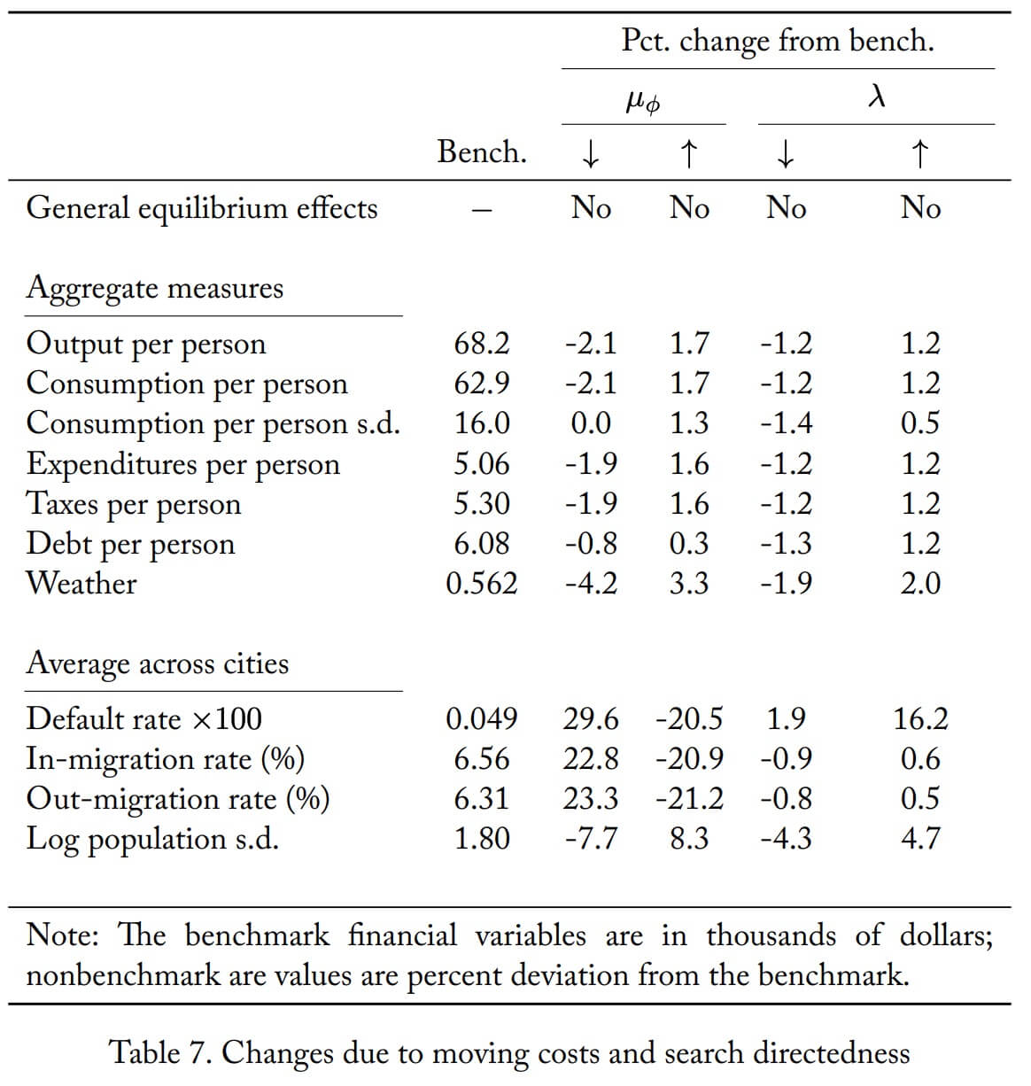
Optimal borrowing limits?

With a better understanding of the model mechanisms, we now turn to the model’s counterfactuals. One prediction of the theoretical model is that a supralocal government may wish to constrain local government borrowing. And, as we showed, CA, MI, and several other states have imposed municipal borrowing limits. Using the model, we now explore what would be the impact of lifting these limits by setting δ to a large value. In contrast to the earlier exercise (in the previous subsection), we allow for general equilibrium effects. The results are displayed in column δ = ∞ of Table 8.

To understand why output goes down, one must remember there are essentially two types of cities in the model: cities constrained by the exogenous borrowing limit and cities constrained by the private credit markets. The first tend to be high-productivity cities (because their bond prices are better) while the latter tend to have low productivity. By eliminating the exogenous limit, high-productivity cities accumulate more debt. This reduces household incentives to relocate to high-productivity cities, which results in lower output. Everything that comoves with output, such as consumption, expenditures, and taxes, also falls. Moreover, welfare, as measured by J (see equation 10), also falls (because J is negative in the benchmark, a positive percent change means a lower J). At face value, this measure—which is potentially problematic as it ignores transition costs—indicates that borrowing limits are in fact optimal. However, the magnitudes of the changes are small because, as previously discussed, private credit markets significantly constrain city borrowing.

A return to high interest rates

In light of the recent increases in the federal funds rate, we assess the impact of a higher risk-free rate on municipalities. In particular, we increase the risk-free interest rate in the model from 4% to 6.5%—the latter corresponding to the interest rates in the early 1990s as can be seen in Figure 2—by reverse-engineering a risk-free bond supply B that delivers a 6.5% interest rate. The results are displayed in Table 8 in the column labeled q −1 ↑.

More expensive borrowing reduces the incentives to issue debt, and debt per person declines by 16%. The higher debt service costs encourage migration away from high-debt, low-productivity cities, which increases aggregate output and “weather” slightly (both of which only reflect sorting). Naturally, then, consumption also increases.²⁸ Default rates fall slightly in the long run, while still remaining low overall.

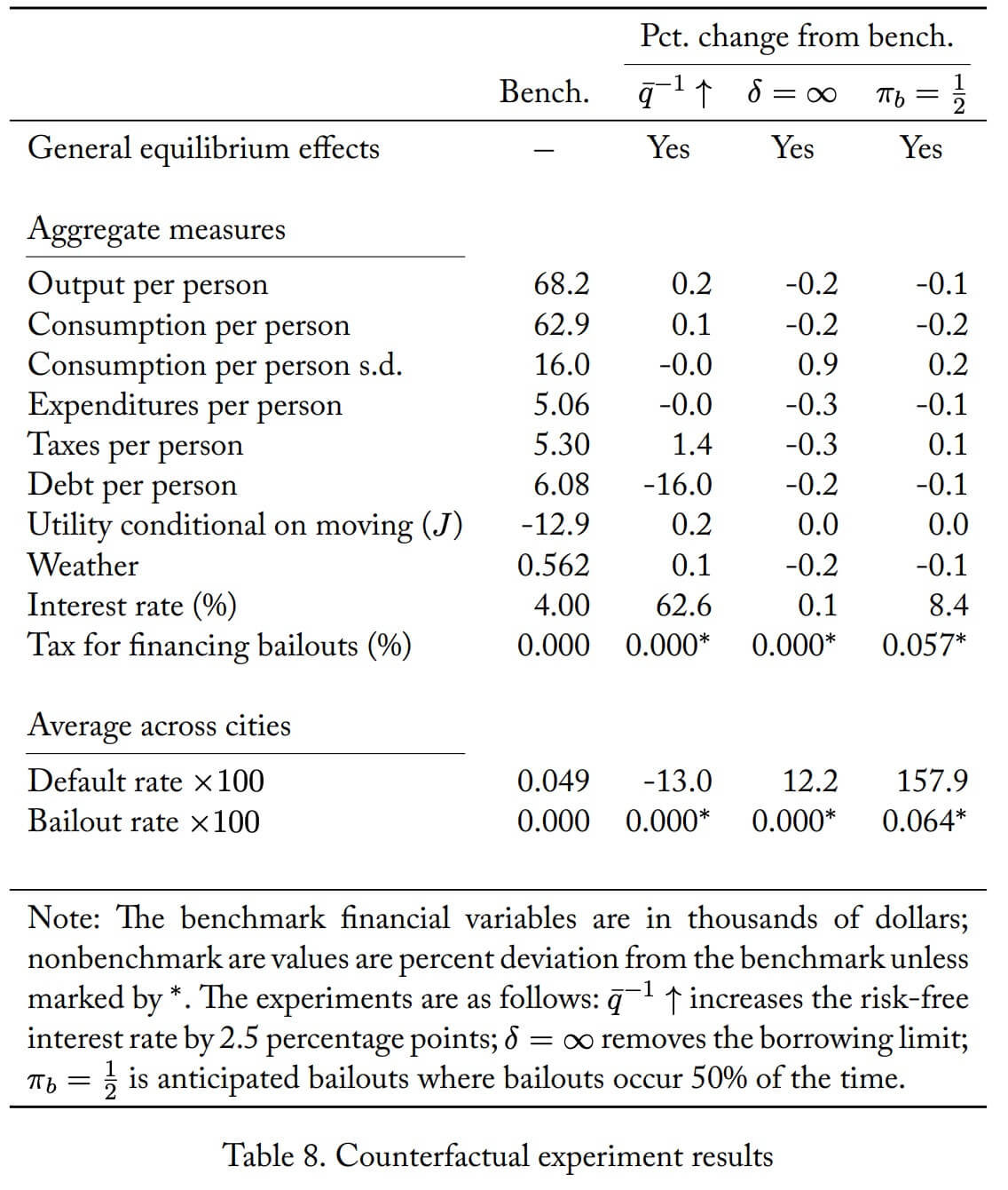
From these results, we conclude that, while there will be some effects from a return to high interest rates, the overall impact is likely to be small, at least in the long run.

What should Detroit have done differently?

Since our model has city planners who maximize the welfare of current residents, the planner’s response to shocks gives an optimal strategy for dealing with adverse (or beneficial) shocks. Hence, by feeding Detroit’s observed shock path into our simulation, our model provides a counterfactually optimal path for the city including policy prescriptions.²⁹ We conduct this simulation by feeding in the estimated fixed and residual productivity series when starting the economy with the initial debt and population observed in the data. (For robustness, Appendix D.8 gives the paths where the simulation starts after a long burn-in.)

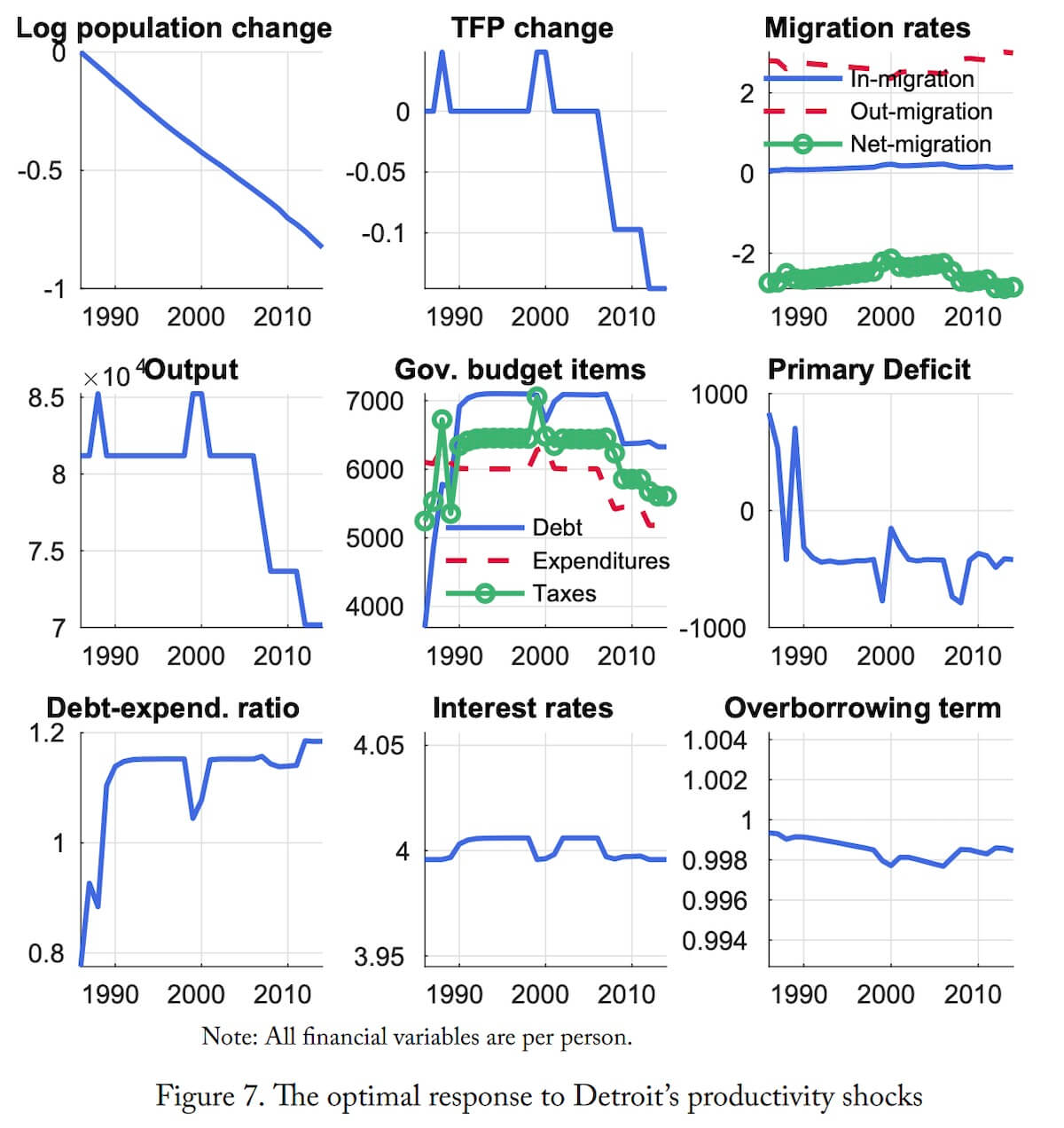
The simulation results for Detroit are displayed in Figure 7, and they show that Detroit’s model-implied long-run level of population is much lower than its 1986 level. From 1986 to 2011, the model predicts a 0.75 log decrease or a 53% decline in population. While the decline in the data over this period was 0.45 log point or 36% (see Figure 2), we note that Detroit’s population has continued in its downward march in the data. In the model, the levels of debt, expenditures, and taxes stabilize after a few years of debt accumulation, and the city then optimally runs a primary surplus of around $500 per person. The optimal model-implied debt level in the early 2000s of around $7,000 per person is not far from the value Detroit actually held, which was around $7,000 in 2001. However, Detroit’s debt continued to grow, and at the start of the financial crisis was around $10,000 per person. More importantly, when productivity sharply fell in the financial crisis, precipitating the General Motors bankruptcy, the optimal response was to cut expenditures and—to a lesser extent—taxes, reducing debt per person by $750. In contrast, Detroit raised taxes and expenditures simultaneously, ultimately increasing debt per person by $2,500.

While Detroit is a special case in terms of the magnitude of changes it underwent, its suboptimal response to adverse productivity shocks is not. In particular, one signficant disagreement between the model and data is the correlation between deficits and out-migration. In the fixed-effects regressions of Table 1, the negative correlation between between deficits and out-migration is only weakly negative. Emblematic of this weak correlation is that Detroit’s out-migration in the financial crisis was paired with larger deficits (as seen in Figure 2). In contrast, the same fixed-effects regressions on model data (in Table 5) reveal a strong negative correlation between deficits and out-migration: when adverse shocks hit and increase out-migration, the optimal response is to significantly deleverage. While Detroit’s residents in the model unanimously favor the record primary surpluses of $800 per person, one can see that in practice these policies would not be particularly popular, especially at a time when output has fallen by more than $10,000 per person.

Bailouts (or, what should the U.S. have done differently?)

The dire effects of the financial crisis not only precipitated Detroit’s bankruptcy, but also led to bailouts for General Motors and Chrysler. This led to discussion on whether Detroit should be bailed out, to which the governor of Michigan replied “bankruptcy is there to deal with the debt question” (Condon, 2013). Moreover, bailouts are not just a Detroit issue. For instance, Hartford’s finances exhibit massive swings in expenditures while taxes and debt are steady (as can be seen in Figure 2) because of repeated, but uncertain, cash infusions from the Connecticut state government. We now examine a general bailout policy that applies to any city at risk of default. Specifically, we will focus on ε-bailouts as made precise by the following definition:

Definition 2. An ε-bailout is an unconditional transfer of resources b (measured per person and after migration) that makes the government indifferent between repaying and default (and we assume they repay in such a case). Formally, b(x) is given by S N ( ˙b(x) + b(x), n˙(x), z, ω) = S D( ˙n(x), z, ω).

We assume bailouts occur with probability πb (i.i.d.) known to the local government. We also assume that households make migration decisions before seeing whether the city is bailed out or not. Hence, n˙ and ˙b are functions of x (as before) and do not depend on whether a bailout is realized or not. To pay for the bailouts, we suppose a federal government taxes purchases of the risk-free bond at rate τ . These assumptions change debt pricing and the intermediary’s problem. They also require a federal government budget constraint. We describe these modifications in Appendix D.5.

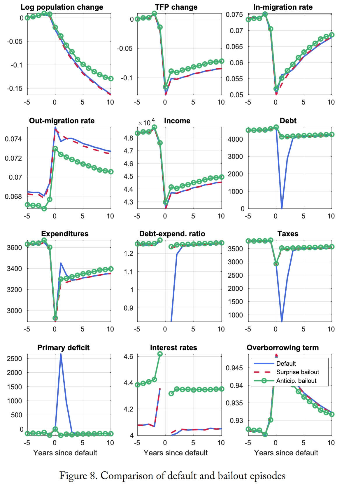
As can be seen in column πb = 1 2 of Table 8, anticipated bailouts that occur with 50% probability more than double default rates. However, apart from this change, the effects on the other statistics are quite weak with output, consumption, and expenditures all falling. Again, the exogenous borrowing limits play a significant role: cities would like to borrow significantly, but loosening the borrowing constraint by increasing expenditures (at the expense of consumption) is distortionary. Additionally, with ε-bailouts, utility in the bailout period is the same as utility in default, which is very low. This also limits any utility gain from being bailed out to excessive spending in the periods leading up to the bailout.

To examine the moral hazard effects, we again turn to default episodes. These are displayed in Figure 8, which plots the benchmark’s default (blue lines) and anticipated bailout (green circled lines) episodes, as well as surprise bailouts (red dashed lines) that are measure zero events. Anticipated bailouts do not lead to excessive borrowing as cities at risk of default are already at or very near to their borrowing limit. The surprise bailouts, which show just the cash-injection effects without any moral hazard or general equilibrium effects, reveal effects on debt, taxes, expenditures, and deficits, but all those changes do little to change the population dynamics. Overall, we find the effects of ε-bailouts to be quite small.

Conclusion

Borrowing, migration, and default are intimately connected. Theoretically, we demonstrated that migration tends to result in overborrowing. Empirically, we documented that defaults can occur after booms or busts in labor productivity and population, that in-migration rates are negatively correlated with deficits, and that many cities appear to be at or near state-imposed borrowing limits. We interpreted these empirical findings loosely in light of the theoretical results, but our quantitative model was able to formalize these explanations by replicating these and many other features of the data.

Our counterfactuals revealed a number of interesting results. One novel result was that Detroit should have cut spending, taxes, and debt in response to its large negative TFP shocks in 2007, 2008, and 2009, thereby avoiding default. We also found that bailing out Detroit and cities like it does not generate large moral hazard costs as long as the bailouts are not generous. With regards to monetary policy, we found a return to a high interest rate environment, while slightly improving GDP via migration incentives, has fairly small effects. Last, we found that eliminating state-imposed borrowing limits should have small effects because private credit markets restrain cities nearly as much as the state-imposed limits.

While our paper has focused on municipalities, it should also prove useful for analyzing states and nations. The drastic population flight from Puerto Rico, a less well-known population decline in Greece, and large in-migration to Spain are three such applications where our framework could prove useful.

On Regional Borrowing, Default, and Migration

Executive Summary

Resources

Focuses

States

Introduction

On borrowing and migration