Are Marijuana and Alcohol Substitutes?

1. Introduction

While marijuana legalization spreads rapidly across the United States (eleven states now allow recreational consumption) and globally (Canada and Uruguay have fully legalized marijuana), many questions about the public health risks remain. Is marijuana legalization responsible for recent increases in traffic fatalities (Aydelotte et al. 2017; Hansen et al. 2019b)? Is the relative risk of marijuana-impaired driving similar to that of drunk driving (Levitt and Porter 2001)? If so, what are the right legal thresholds for impaired driving and what are the optimal punishments (Hansen 2015)? The answers to all of these questions directly or indirectly depend on the answer to the underlying economic question that medicine, economics, and public health have long debated: are alcohol and marijuana substitutes or complements (or perhaps neither)?

The empirical literature remains divided, although recent evidence has mostly found that the goods are substitutes. Microlevel data on the goods’ consumption reveal strong positive correlations among young users (Bruns and Geist 1984; Collins et al. 1998). Those who consume marijuana often also consume alcohol. However, despite this strong correlation, it could be that people are heterogeneous in their preferences. Some people like drugs (both legal and illegal) and some do not. If this is true, then cross-sectional comparisons might reveal relatively little about the effects of changing the price, including distance, time, or other latent costs, of other goods while holding all else constant.

In a simple model of economic substitutes and complements, all we need is price variation to learn the cross-price elasticity. However, in the real world, price variation is often driven by endogenous demand shocks. While medical marijuana laws have been followed by price decreases in high quality marijuana 3-4 years following legalization, those laws affect both the demand for and supply of marijuana (Anderson et al. 2013). Moreover, some recent papers have found evidence of substitution (Anderson et al. 2013; Crost and Guerrero 2012; Kelly and Rasul 2014) while others suggest complementarity (Pacula 1998; Williams et al. 2004; Wen et al. 2015). It might seem natural to test whether marijuana affects alcohol consumption by studying states that have legalized. However, such states all had preexisting medical marijuana regimes. Thus, it’s possible in the short run that legalization mostly cause substitution in recreational use between sources, as people shift from black market and medical marijuana to recreational options. However, in nearby regions, the new recreational marijuana markets could decrease the opportunity cost of purchasing marijuana. In this paper, I focus on border spillovers and the plausibly exogenous shift in the opportunity cost of purchasing marijuana that a neighboring state’s legalization could represent.

Prior research has found that consumers can be sensitive to small differences in local prices, which are often induced by differences in local taxes or by purchase bans (Asplund et al. 2007; Shelley et al. 2007). The incentives are even stronger for sin goods because they represent a large share of income for many frequent users and because they have a fairly long shelf life. Through studying sales patterns or collecting cigarette packs from the garbage, researchers have demonstrated consistently that cigarette consumers cross-border shop (Harding et al. 2012; DeCicca et al. 2013). Changes in alcohol prices are less common in the United States, so instead Lovenheim and Slemrod (2010) focus on the minimum legal drinking age (MLDA) and find evidence that young adults cross borders to purchase alcohol in jurisdictions where they have legal access. Moreover, Stehr (2007) finds that people drive to the county next door to purchase alcohol in response to a Sunday liquor ban, despite its temporary and predictable nature.

In July 2014, recreational marijuana retailers opened in Washington State. For many residents of Idaho, this made purchasing marijuana easier and legal. Additionally, this shift in access was plausibly exogenous to Idaho residents, where marijuana remains illegal for any use. Oregon then legalized recreational sales in October 2015. However, local jurisdictions had control over whether legal sales could occur within their borders. This led to an effective ban on marijuana sales in nearly all of Eastern Oregon until 2016. In March 2016, two retailers in Huntington, Oregon, opened, with local officials openly admitting that this decision was driven by the desire to attract buyers from Idaho. Subsequently more retailers open in Ontario given the substantial demand and the financial local benefits of additional excise tax revenue. This series of expansions to legal access in close proximity to Idaho provides a unique natural experiment for testing whether alcohol and marijuana are substitutes. Recent research by Hao and Cowan (2017) and Hansen et al. (2019a) finds evidence that consumers from neighboring regions purchase marijuana in Colorado and Washington.

This study is the first to focus on the health externalities of this cross-border shopping and whether this increased or decreased traffic accidents related to alcohol abuse. I find evidence that searches for “dispensaries,” a term for stores selling marijuana, increased dramatically in Idaho following legalization. Further, state police seizures of marijuana on highways increased from only thirteen in 2013 to over eight hundred in 2018. Moreover, drunk-driving-related accidents per vehicle mile traveled (VMT) fell following Washington’s dispensary openings. Finally, I use administrative data on traffic accidents from 2010 to 2017 in Idaho. I find that alcohol-related accidents fell following Washington’s legalization but that this decrease differed in absolute magnitude depending on the distance to the border, with the largest decreases in the regions closest to marijuana retailers.

In section 2, I discuss the timeline of legal access and Idaho’s current legal treatment of marijuana. In section 3, I review the data and empirical methods I use. I discuss the estimated models in section 4. In section 5, I reach conclusions and discuss policy implications of my results.

2. Background

Federal prohibition of marijuana began in 1938, though Idaho, Washington, and Oregon had banned marijuana in 1927, 1923, and 1923 (Sanna 2014). While laws have been liberalized in Washington and Oregon—with legalization for medical use in both states in 1998 and legalization for recreational use more recently (2012 and 2014)—Idaho is one of the few states that do not allow marijuana possession for medical or recreational use. When legal sales began in Washington in July 2014, retailers opened in Spokane and Walla Walla and those became the closest sources of consumer marijuana (as opposed to black market marijuana) for residents in Idaho. Oregon followed Washington by allowing commercial sales of marijuana in October 2015. Legal sales in Oregon began in 2015 months before licenses were granted because of an emergency bill that allowed all medical stores to sell recreationally. However, local jurisdictions could opt out of allowing local sales, and essentially all of Eastern Oregon chose to ban local sales. As one can glean from Pacula and Sevigny (2014) and Anderson et al. (2014), it can be challenging to learn from policies with staggered rollouts.

In 2016, two marijuana retailers opened in Huntington, Oregon. This is noteworthy because the town abuts I-84 and is a little over an hour from Boise (while Walla Walla and Spokane are four and seven hours away). Moreover, despite Huntington’s population being only 440 in the 2010 Census, the two marijuana retailers have a combined total of 2,844 reviews online. The high number of reviews relative to the population size suggests many consumers are likely coming from other regions, with the largest population center nearby being Boise, Idaho. July 2014 is when sales became legal in Spokane, Washington. Sales began in Walla Walla, Washington, in September 2015 and in Huntington, Oregon, in March 2016. These are the key dates that could affect the opportunity cost to Idaho residents of purchasing marijuana.

Prior research suggests that cross-border shopping for marijuana is substantial. Based on the local population sizes relative to local sales, Hansen et al. (2019a) estimate that 24 percent of recreational marijuana sold in Spokane, Washington ends up in Idaho, and that potentially 90 percent of marijuana sold in Huntington or Ontario is purchased by Idaho residents. Hao and Cowan (2017) find evidence that marijuana arrests increased in neighboring regions, including Idaho, following legalization in Washington and Colorado. Whether a person in Idaho will purchase marijuana where she has legal access of course depends on her trade-offs and opportunity costs. Black market marijuana remains available in Idaho. And driving to a nearby state, purchasing marijuana, and bringing it home is a crime in its own right. More generally, whether people choose to cross-border shop for legal marijuana depends on several factors: the price, the distance traveled, the likelihood and consequences of being searched by state police, the perceived value of legal markets (and risks in black markets). Many of these trade-offs relate directly to the legal regime in Idaho.

Marijuana possession remains illegal in Idaho. If the amount is less than three ounces, it is a misdemeanor that could result in up to a year of jail time. Possession of any amount over that is a felony. Possessing of or transporting over one pound is a felony punishable by a minimum prison sentence of one year and a $5,000 fine. Trafficking over five pounds results in a minimum prison sentence of three years and a $10,000 fine, while any trafficking more than twenty-five pounds carries a prison sentence of at least five years and $15,000 in fines.¹Anderson, Mark D., B. Hansen, and D. I. Rees. 2013. “Medical Marijuana Laws, Traffic Fatalities, and Alcohol Consumption.” Journal of Law and Economics, 56 (2): 333–69. Notably, none of these policies have changed in recent years.

The Idaho State Police have reported consistent increases in trafficking and seizures following Washington’s and Oregon’s legalizations. However, what remains unknown is whether the marijuana purchased in neighboring regions has been significant enough to affect public health outcomes such as traffic injuries. It could be that legal cross-border marijuana sales crowd out black market marijuana sales. And whether such sales increase or reduce traffic accidents depends on the substitutability or complementarity between alcohol and marijuana.

3. Data and Methods

I use several sources of data to measure the demand for marijuana, the degree of cross-border shopping by Idahoans, and the spillover impacts on public health. Below I describe the key data sets and empirical approaches I use.

3.1 Measuring Marijuana Demand in Idaho

Measuring local marijuana demand is always challenging. The National Survey of Drug Use and Health provides state-level estimates of lifetime and recent marijuana use at the state level. However, the questions it asks are not well suited to measuring daily or extensive marijuana use as they focus on whether someone has consumed marijuana in the last thirty days rather than how many times. Indeed, health surveys in the United States miss the right tail of drug use, as shown in Carpenter et al. (2016).² These problems are exacerbated in the substate measures, which rely on three- to five-year moving averages and hence are poorly suited to picking up immediate changes resulting from policy shifts.

With that in mind, I focus on proxies for marijuana interest based on Google keyword searches. Many other recent papers have shown Google searches can offer reasonable proxies for latent demand or interest (Schaller et al. 2017; Oster 2018). I focus on Google searches for the word dispensary. Searches for other words such as marijuana could increase with marijuana legalization but are probably split between those who want to buy it and those concerned about its potential harms. People likely search for dispensary, on the other hand, when they want to go to a dispensary, which we would expect when they want to buy marijuana. Notably, one open question is whether we are measuring a news response—that is, searches in response to headlines. Prior work by Schaller et al. (2017) and Oster (2018) suggests news-related spikes are likely short lived. Thus any headline effects should manifest themselves in the raw trends.

Google Trends is an online tool that reveals the relative frequency of Google searches across space and time. Results represent relative interest, where 100 indicates peak interest and 0 indicates minimal interest. To measure how interest shifts, I use an interrupted time series approach based on monthly data from 2007 to 2017. The estimated effect of nearby access on interest in dispensaries is based on equation 1.

(1)  

measures whether searches jumped noticeably the month marijuana became recreationally available in Washington, and measures whether the trend of marijuana interest shifted, allowing for a gradual change in interest. I also estimate a similar model for police searches with the number of marijuana seizures as the dependent variable.

3.2 Measuring Public Health Spillovers

To test whether recreational marijuana sales in nearby regions decrease drunk driving, I use data on traffic accidents from Idaho’s department of transportation. I focus on data from 2010 to 2017, which includes four years of pre-treatment and four years of post-treatment analysis. I focus on these years to avoid the potential influence of the Great Recession, as traffic accidents fell considerably during the years 2007–9. While the federal government collects information on all fatal accidents in the Fatal Analysis and Reporting System, I focus on all traffic accidents. Given Idaho’s relatively small population, including accidents causing property damage, injury, and death provides considerably more statistical power than examining only fatal accidents. Alcohol-related crashes tend to be more severe and are more likely to involve injuries and death than crashes that do not involve alcohol. Also, as shown in table 1, marijuana-related accidents are quite rare in Idaho, perhaps because blood tests are infrequent. Accordingly, I focus on alcohol-related crashes in this study, but marijuana-related crashes merit more attention in future research.

In my models, I focus on whether alcohol-related traffic fatalities shifted followed marijuana legalization in Washington in 2014. As shown in figure 1, the fraction of accidents involving alcohol dropped significantly. Moreover, the count of alcohol-related crashes per VMT fell. These patterns are certainly suggestive of potential substitution between alcohol and marijuana, but they could also just capture a continuation or acceleration of earlier trends. To estimate the effect of nearby marijuana access, I use models that are similar to a difference-in-difference design but allow for treatment to be defined continuously. This is because while theoretically anyone in Idaho could travel to Washington to purchase marijuana, the time costs vary considerably between people on the border, within an hour of retailers, and those in other parts of the state, up to a day’s drive (eight to nine hours) away. This is depicted in figure 2, which shows dispensaries in Washington and the two along the border in Oregon and the average distance to a dispensary from 2014 to 2017. There is substantial variation within the state cross-sectionally and over time based on whether the dispensaries were allowed to sell recreationally.

I estimate the variation with models that include county fixed effects (), a dummy variable for recreational marijuana legalization nearby, , and the interaction between the average driving time (in hours) between a county and legally available marijuana, . Distance is measured by the number of hours (at average speeds) it takes to drive from a county centroid to the closest marijuana retailer. The distance between a county and legal access does not enter the model as it is time invariant because the model includes county fixed effects. The coefficient on the interaction is similar to that in a difference-in-difference model in which treatment is continuous. If marijuana and alcohol are complements, then alcohol use should increase with marijuana legalization, but this effect should dampen with distance (meaning the coefficient on the interaction would be negative). On the other hand, if marijuana and alcohol are substitutes, should be negative and positive, as individuals decrease their alcohol consumption close to the border but less so (approaching zero) further away from it.

(2)  

In addition to the baseline model in equation 2, I also estimate a more generalized model in equation 3. The key difference is that instead of there being an interaction between a single dummy variable for the period following recreational marijuana legalization nearby, there is a vector dummy variable for each year, and those variables are interacted with the distance to nearby legal recreational marijuana (with the year prior to legalization being omitted). In this model, the vector can broadly show that the trends of drunk driving are varying from their original 2010 levels, while the coefficients on the vector tell us whether those trends differ based on the distance to legally available marijuana. If legal recreational marijuana access reduces drunk driving, we expect the coefficients on the dummy variables for each year will turn negative and the interactions between the dummy variables for year and distance will only turn positive for 2014 and later.

(3)  

I also include controls for local economic conditions largely because both alcohol consumption and traffic accidents have been shown to be procyclical (Ruhm, 2000; Ruhm & Black, 2002).

In addition to the models examining how drunk driving as a share of total traffic accidents shifts, I also examine the count of drunk driving accidents. A chief challenge in examining the count of traffic accident is the role of VMT. Idaho only provides official estimates of VMT at the state level. However, it also provides measures of average daily traffic (ADT) based on automated road counters, which is proportional to VMT as long as individuals tend to drive the same set of roads. Thus I used ADT as a proxy for VMT, which is more commonly used in transportation research.

To measure the effect of nearby legal marijuana access on the count of drunk driving accidents, I use Poisson fixed effect regressions. The specifications are similar to the linear models above. The key difference in the Poisson models is the assumption about the conditional mean of the outcome. The Poisson models assume . So these regressions are similar to linear regressions with a logged outcome variable, but they allow for cases in which there are zero accidents. ADT is used as an exposure variable in the Poisson regression, as I assume that accidents increase proportionately with traffic flows. In other words, is included as a regressor with its coefficient constrained to be 1. For the Poisson regressions I report incident-rate ratios. The estimated ratio minus 1 indicates the percentage shift. For example, an incident-rate ratio of 1.10 indicates a 10 percent increase, while a ratio of 0.90 indicates a 10 percent decrease.

4. Results

In this section, I explore both the proxies for interest in nearby marijuana and the effect of nearby marijuana access on local traffic accidents.

4.1 Marijuana Interest in Idaho

As explained in the prior section, I use proxies for marijuana interest via Google searches from Google Trends and data on marijuana searches and seizures from the Idaho State Police. I test for the effect of marijuana access on interest by estimating interrupted time series and examining whether interest shifts both in the intercept and in trend following legal access. The key points of legal access are when marijuana stores opened in Washington’s Walla Walla and Spokane in July 2014 and when stores opened in Huntington, Oregon, close to Boise.

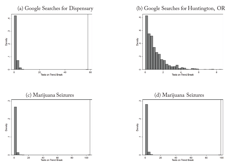
Figure 2 shows the time series of Google searches and the number of marijuana drug seizures in Idaho surrounding legalization in the nearby states. In each plot, it seems as though the time series trend breaks upward and potentially jumps after the onset of nearby marijuana access. This suggests interest in nearby marijuana increases with legalization. Notably, the effect of news stories should be manifested through short-term increases in searches, but we don’t see such increases. Searches for “Huntington, Oregon” (which someone might type into Google before driving there) increase notably after sales begin in Huntington. The same is true for searches for “Huntington Dispensary.”

Table 2 reports the estimated coefficients on the regression models testing for an interrupted time series. In all the models, both the coefficient on a dummy variable measuring marijuana access and the coefficient on trend interaction with the access variable are large, positive, and precisely estimated, resulting in a high degree of statistical significance.

It’s possible that the above results are due to misspecification. Indeed, time series data are often autocorrelated, and the trends might be nonlinear or a linear trend might not be constant over time. To test whether a regime change really occurred or the coefficients are just detecting a nonlinearity, I perform randomization inference with the date reshuffled and the test redone on the regime with the randomized date. Appendix figure 1 contains a histogram with reported test statistics from an F-test on whether the coefficients on marijuana access and on marijuana access interacted with the linear trends are equal to zero. The vertical line represents the F-test from the original model without randomization. As is evident from the figures, the F-test from the true time variables is one of the largest, if not the largest, values in the distribution. The implied p-values, reported in table 2, range from 0 to 0.001 for the various marijuana proxies I examine. This suggests that interest in marijuana—specifically, marijuana available in Washington and Oregon—increased significantly as stores opened nearby and that the trend break is not due to random chance.

4.2 Public Health Spillovers

4.2.1 Linear Regressions

I first examine the effect of legal access to marijuana and its interactions with distance in linear regression models. These models capture whether alcohol use as a contributing factor in traffic accidents decreases or increases in relative incidence following marijuana legalization and whether those effects vary based on distance to nearby recreational marijuana access.

Table 3 reports the estimated effect of recreational marijuana access with distance interactions. The first model in column 1 includes distance as a linear variable (in hours). The model in column 2 includes the natural log of travel time. The model in the third column uses a partial-treatment variable, estimates of which would take on a value of 1 with zero distance to treatment (next door to a dispensary) and decline quadratically from there. I anticipate that if marijuana access decreases drunk driving in counties close to recreational marijuana stores, the interaction should be positive for the linear time measure and its log in columns 1 and 2 and negative for the partial-treatment measure in column 3.

The point estimates in Table 3 suggest that recreational marijuana legalization decreases the fraction of accidents involving alcohol by 0.005. Given that the original average prior to marijuana legalization in border counties was 0.023, this represents a 21 percent decrease. It’s worth noting the symmetry between the point estimates for coefficients on Legal in columns 1 and 2 and the partial-treatment interaction in column 3. That symmetry appears because each model is attempting to measure the same policy parameter, the effect of marijuana access if distance is reduced to zero. The decrease in drunk-driving-related accidents is consistent with substitution away from alcohol and to marijuana, at least on average.

There are no locations in Idaho with zero distance to marijuana retailers. Thus what matters is the linear combination of the coefficients on Legal and the distance interactions. Those estimated partial effects are provided in the final three rows of table 3. At one hour away, the point estimates from the various models suggest the fraction of accidents involving alcohol decline by 0.0042 to 0.0045, or roughly 18 percent. At three hours, the point estimates from the various models suggest a decline of 0.002, or roughly 10 percent. Finally, at six hours the estimates vary from −0.001 to 0.002. At those distances I am unable to reject the null hypothesis that the effect becomes negligible when the driving distance is more than a day away.

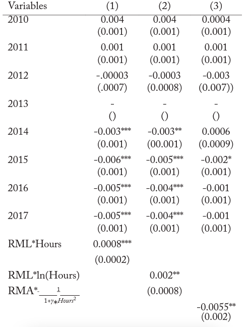
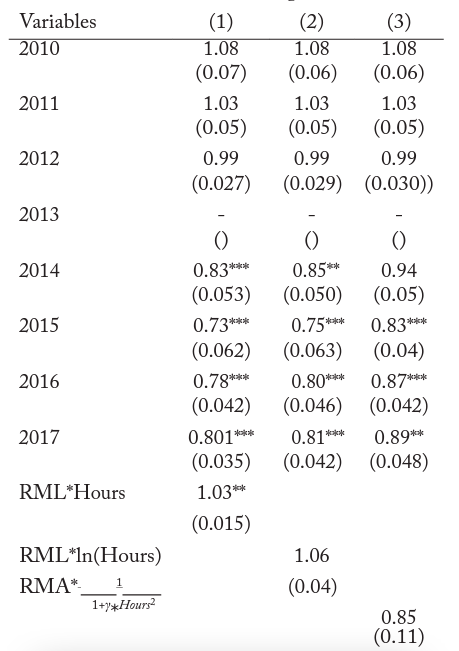
Table 4 presents regressions that allow for a more generalized structure. Rather than a simple dummy for legal access to marijuana, the models presented in table 4 use dummy variables from 2010 to 2017, omitting 2013 as the base year. This offers a partial test of the common-trends assumption inherent in any difference-in-difference design. The prior models might have been biased if the regions closer to marijuana stores were on a different trend than the rest of the state or if alcohol-related accidents were falling prior to marijuana access. If the interactions with distance to the border are large and significant during the pre-treatment period, this suggests the regions close to marijuana stores were likely on an entirely different trend prior to legalization. While the common-trends assumption during the post-treatment period remains untestable, this event-study test offers a necessary condition to interpret the prior estimates as causal.

As shown in table 4, the point estimates for the dummy variables on the years 2010–12 are all small and statistically insignificant. This offers evidence that the counties across Idaho have similar trends regardless of their distance to the border. Only in 2014 do the estimates become negative, which then is offset based on the interaction between distance to border and the year dummies. The estimated coefficients from these models again suggest that access to marijuana from nearby legalization reduces the fraction of accidents associated with alcohol but that those effects are smaller with distance.

4.2.2 Poisson Regressions

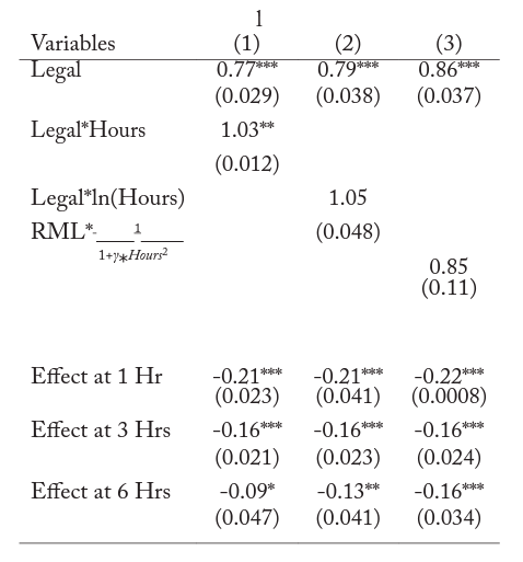
The prior analyses based on linear regression focused on the fraction of accidents involving alcohol. Inasmuch as accidents, both alcohol related and not alcohol related, are proportionate to VMT, these models suggest alcohol and marijuana are substitutes. Another approach is to examine how the count of traffic accidents involving alcohol shifts following legalization. Poisson regressions are well suited to this approach given the count nature of accidents and the absence of alcohol-related accidents in some county–year pairs. The scaled point estimates for Poisson regression models are reported in table 5. As noted earlier, ADTs are included as an exposure variable. The estimates are scaled to represent incident-rate ratios. A ratio larger than 1 indicates an increase, while a ratio less than 1 indicates a decrease. The point estimates on Legal are consistently negative, suggesting that access to marijuana brought about by legalization in neighboring jurisdictions results in a 23 percent decrease in alcohol related crashes. As shown in columns 1 and 2, the estimated effects fall with distance. Each hour reduces the estimated effect of legal access by 3 percent. As shown in the final three rows, the net estimated effect becomes much smaller for regions further away. The quadratic inverse distance measure again suggests the effect decays nonlinearly. One complication for the inverse distance measure is the necessity of a nuisance parameter. In this particular case, I assume a value of the parameter such that one hour away, the effective access of marijuana one hour from the border is 62 percent of the access offered in regions with legal recreational sales, motivated by the spillovers estimated in Hansen, Miller and Weber (2018b). In table 6, I explore the time trends of accidents more flexibly, as in table 4. Again, it appears that the count of accidents involving alcohol falls in the period following marijuana legalization but that these effects vary with distance. The interactions with distance (presented in the final three rows of the table) suggest that the effect of legal access on alcohol-related crashes diminishes by roughly 3 percent for each hour of distance from a retailer.

5. Conclusions

Support for marijuana legalization has hit record highs recently, with 65 percent favoring it (Kellam 2019). Even overwhelmingly conservative states, including Utah and Oklahoma, have passed medical marijuana laws, and one in four Americans can legally purchase marijuana for recreational use as of November 2019. Despite this broad increase in public support, there remains a large gap across generations and political affiliation, and in many regions marijuana is illegal for medical and recreational uses. Two of Colorado’s neighbors sued the state for a share of its marijuana tax revenues to offset their increased enforcement costs. The increase in enforcement of marijuana trafficking laws is clear for states such as Idaho, where thirteen people were arrested for smuggling marijuana in 2013 but over eight hundred were in 2018.

One of the continued points of discussion involves the externalities of increased drug use, particularly in states where it remains illegal. The potential externalities in those states are all the more relevant because those states have not collected tax revenues, which would typically offset the externalities. While prior research has suggested a nontrivial number of people may be cross-border shopping to purchase marijuana in legal areas, this research is the first to attempt to quantify these externalities through measuring risky driving (Hao and Cowan 2017; Hansen et al. 2019a).

Based on an interrupted time series using proxies for consumer interest, I find evidence that Google searches related to marijuana access increase with the availability of nearby marijuana retailers across state lines. Using a generalized difference-in-difference design, I estimate the effect of marijuana access on alcohol-related traffic accidents. Using the difference in treatment that distance implies, I find evidence that marijuana legalization results in an 18 percent decrease in alcohol related accidents among residents of Idaho within an hour of a marijuana retailer. This effect diminishes with each hour of distance (one way) such that after the distance reaches three to four hours the effect become negligible.

Future research should address the external validity of these effects in other regions of the country affected by marijuana legalization. For instance, recent reports suggest that New Yorkers are driving hours to Massachusetts to purchase legal marijuana (Slattery 2019), and Hansen et al. (2019a) find that over 70 percent of border sales in Massachusetts can be attributed to out of state buyers. Other negative externalities such as injuries resulting from marijuana-related traffic accidents, which I didn’t capture in this study, also might increase.

6. Figures and Tables

Figure 1. Alcohol-Related Crash Trends in Idaho

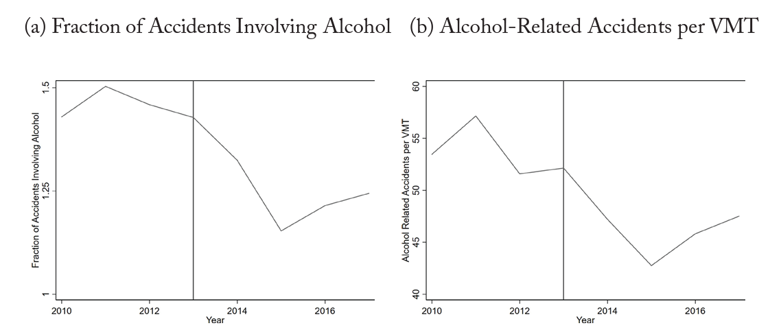
This figure shows the fraction of accidents involving alcohol, on the left, and alcohol-related accidents per VMT, on the right. Data for both come from Idaho accident reports from 2010 to 2017.

Figure 2. Idaho and Distance to Nearby Dispensaries by County

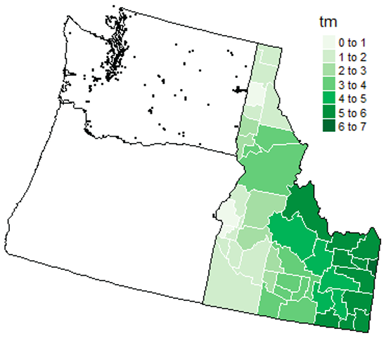
This figure shows the average distance to a nearby dispensary during the period 2014–17 by county in Idaho.

Figure 3. Marijuana Proxies based on Searches

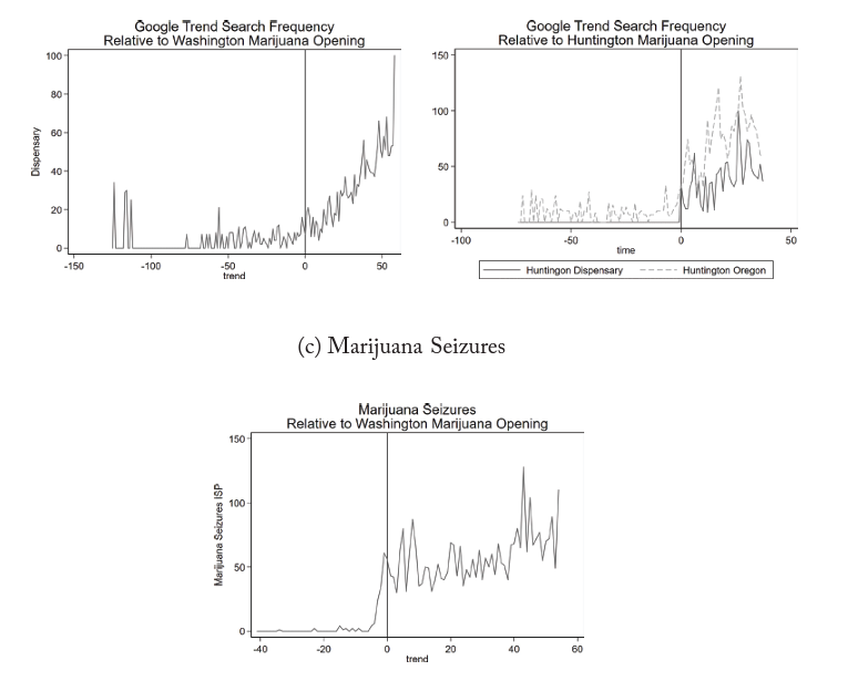
This figure shows proxies for marijuana interest. Panel A is Google searches for “Dispensary,” with the vertical line representing Washington legalization. Panel B is searches for either “Huntington, OR” or “Huntington Dispensary,” with the vertical line representing the Huntington store opening. Panel C is searches for marijuana seizures, with the vertical line representing Washington legalization.

Table 1. Summary Statistics

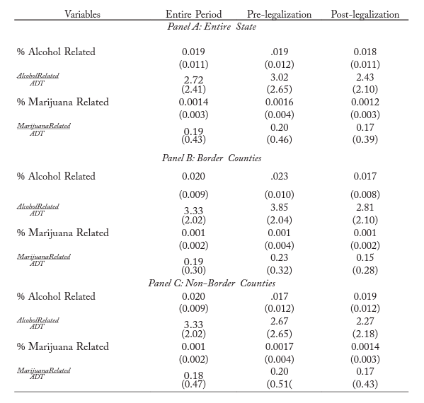
This table provides summary statistics on traffic accidents in Idaho for the entire sample period, the period prior to marijuana legalization in Washington, and the period following marijuana legalization in Washington.

Border counties are those counties that share a border with Washington or Oregon, while nonborder counties are those that do not share a border with Washington or Oregon.

Table 2. Marijuana Interest and Legal Access

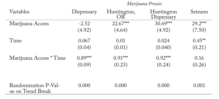
Notes: This table provides estimates of the effect of legal marijuana access interacted with distance to the border. Column 1 is based on hours to the dispensary linearly. Column 2 is based on the ln(hours) to the nearest dispensary. Column 3 is based on the inverse of the distance squared, scaled so that one hour from the dispensary is 0.625 treated, and the effective treatment declines geometrically with distance (three hours is 0.16 treated, and six hours is 0.04 treated. All estimates are based on linear regressions weighted by county population and allowing for clustering at the county level. *, **, and *** respectively indicate significance at the 10, 5, and 1 percent levels.

Table 3. Percentage of Accidents Involving Alcohol

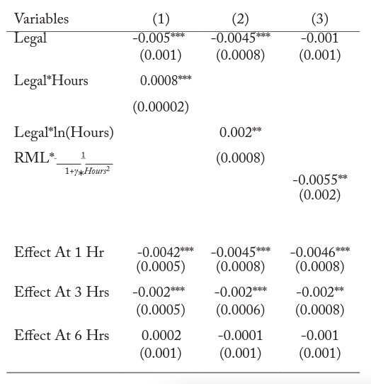
Notes: This table provides estimates of the effect of legal marijuana access on alcohol-related crashes interacted with distance to the border. The dependent variable in each regression is the fraction of accidents involving alcohol. Column 1 is based on hours to the dispensary linearly. Column 2 is based on ln(hours) to the nearest dispensary. Column 3 is based on the inverse of the distance squared, scaled so that one hour from the dispensary is 0.625 treated, and the effective treatment declines geometrically with distance (three hours is 0.16 treated, and six hours is 0.04 treated. All estimates are based on linear regressions weighted by county population and allowing for clustering at the county level. *, **, and *** respectively indicate significance at the 10, 5, and 1 percent levels.

Table 4. Percentage of Accidents Involving Alcohol

Notes: This table provides estimates of the effect of legal marijuana access on alcohol-related crashes interacted with distance to the border. The dependent variable in each regression is the fraction of accidents involving alcohol. Column 1 is based on hours to the dispensary linearly. Column 2 is based on ln(hours) to the nearest dispensary. Column 3 is based on the inverse of the distance squared, scaled so that one hour from the dispensary is 0.625 treated, and the effective treatment declines geometrically with distance (three hours is 0.16 treated, and six hours is 0.04 treated. All estimates are based on linear regressions weighted by county population and allowing for clustering at the county level. *, **, and *** respectively indicate significance at the 10, 5, and 1 percent levels.

Table 5. Count of Accidents Involving Alcohol

Notes: This table provides estimates of the effect of legal marijuana access on alcohol-related crashes interacted with distance to the border. The dependent variable in each regression is count of alcohol-related accidents. Column 1 is based on hours to the dispensary linearly. Column 2 is based on ln(hours) to the nearest dispensary. Column 3 is based on the inverse of the distance squared, scaled so that one hour from the dispensary is 0.625 treated, and the effective treatment declines geometrically with distance (three hours is 0.16 treated, and six hours is 0.04 treated. All estimates are incident-rate ratios from Poisson regressions with county fixed effects, using the average daily traffic count as an exposure variable, and allowing for clustering at the county level. *, **, and *** respectively indicate significance at the 10, 5, and 1 percent levels.

Table 6. Count of Accidents Involving Alcohol

Notes: This table provides estimates of the effect of legal marijuana access on alcohol-related crashes interacted with distance to the border. The dependent variable in each regression is the count of alcohol-related accidents. Column 1 is based on hours to the dispensary linearly. Column 2 is based on ln(hours) to the nearest dispensary. Column 3 is based on the inverse of the distance squared, scaled so that one hour from the dispensary is 0.625 treated, and the effective treatment declines geometrically with distance (three hours is 0.16 treated, and six hours is 0.04 treated. All estimates are based on Poisson regressions with county fixed effects, using the average daily traffic count as an exposure variable, and allowing for clustering at the county level. *, **, and *** respectively indicate significance at the 10, 5, and 1 percent levels.

Appendices

Figure A.1. This figure shows the histogram for the F-statistics whether there was a structural break in the time series for each of the marijuana proxies studied in Table 2. The vertical lines represent the original test statistic before the date was randomized.

References

Anderson, Mark D., B. Hansen, and D. I. Rees. 2013. “Medical Marijuana Laws, Traffic Fatalities, and Alcohol Consumption.” Journal of Law and Economics, 56 (2): 333–69.
Anderson, D. M., D. I. Rees, et al. 2014. “The Role of Dispensaries: The Devil Is in the Details.” Journal of Policy Analysis and Management, 33 (1): 235–240.
Asplund, M., R. Friberg, and F. Wilander. 2007. “Demand and Distance: Evidence on Cross-Border Shopping.” Journal of Public Economics, 91 (1–2): 141–57.
Aydelotte, J. D., L. H. Brown, K. M. Luftman, A. L. Mardock, P. G. Teixeira, B. Coopwood, and C. V. Brown. 2017. “Crash Fatality Rates after Recreational Marijuana Legalization in Washington and Colorado.” American Journal of Public Health, 107 (8): 1329–31.
Bruns, C., and C. S. Geist. 1984. “Stressful Life Events and Drug Use among Adolescents.” Journal of Human Stress, 10 (3): 135–39.
Carpenter, C. S., C. Dobkin, and C. Warman. 2016. “The Mechanisms of Alcohol Control.” Journal of Human Resources, 51 (2): 328–56.
Collins, R. L., P. L. Ellickson, and R. M. Bell. 1998. “Simultaneous Polydrug Use among Teens: Prevalence and Predictors.” Journal of Substance Abuse, 10 (3): 233–53.
Crost, B., and S. Guerrero. 2012. “The Effect of Alcohol Availability on Marijuana Use: Evidence from the Minimum Legal Drinking Age.” Journal of Health Economics, 31 (1): 112–21.
DeCicca, P., D. Kenkel, and F. Liu. 2013. “Excise Tax Avoidance: The Case of State Cigarette Taxes.” Journal of Health Economics, 32 (6): 1130–41.
Hansen, B. 2015. “Punishment and Deterrence: Evidence from Drunk Driving.” American Economic Review, 105 (4): 1581–1617.
Hansen, B., K. Miller, and C. Weber. 2019a. Cross Border Sales, Federalism, and Partial Prohibition: Evidence from Recreational Marijuana. National Bureau of Economic Research.
Hansen, B., K. Miller, and C. Weber. 2019b. “Early Evidence on Recreational Marijuana Legalization and Traffic Fatalities.” Economic Inquiry 0 (0).
Hao, Z., and B. Cowan. 2017. “The Cross-Border Spillover Effects of Recreational Marijuana Legalization.” NBER Working Paper 23426, National Bureau of Economic Research.
Harding, M., E. Leibtag, and M. F. Lovenheim. 2012. “The Heterogeneous Geographic and Socioeconomic Incidence of Cigarette Taxes: Evidence from Nielsen Homescan Data.” American Economic Journal: Economic Policy, 4 (4): 169–98.
Kellam, B. 2019. “Legalizing Marijuana? Americans Support It, but Not Enough to Sway Their Vote in 2020.” CBS News, April 23. 12
Kelly, E., and I. Rasul. 2014. Policing Cannabis and Drug Related Hospital Admissions: Evidence from Administrative Records.” Journal of Public Economics 112: 89–114.
Levitt, S. D., and J. Porter. 2001. “How Dangerous Are Drinking Drivers?” Journal of Political Economy, 109 (6): 1198–1237.
Lovenheim, M. F., and J. Slemrod. 2010. “The Fatal Toll of Driving to Drink: The Effect of Minimum Legal Drinking Age Evasion on Traffic Fatalities.” Journal of Health Economics, 29 (1): 62–77.
Oster, E. 2018. “Does Disease Cause Vaccination? Disease Outbreaks and Vaccination Response.” Journal of Health Economics, 57: 90–101.
Pacula, R. L. 1998. “Does Increasing the Beer Tax Reduce Marijuana Consumption?” Journal of Health Economics, 17 (5): 557–85.
Pacula, R. L., and E. L. Sevigny. 2014. “Marijuana Liberalizations Policies: Why We Cant Learn Much from Policy Still in Motion.” Journal of Policy Analysis and Management, 33 (1): 212.
Ruhm, C. J. 2000. “Are Recessions Good for Your Health?” Quarterly Journal of Economics, 115 (2): 617–50.
Ruhm, C. J., and W. E. Black. 2002. “Does Drinking Really Decrease in Bad Times?” Journal of Health Economics, 21 (4): 659–78.
Sanna, E. 2014. Marijuana: Mind-Altering Weed. Simon and Schuster.
Schaller, J., L. Schulkind, and T. M. Shapiro. 2017. “The Effects of Perceived Disease Risk and Access Costs on Infant Immunization.” Technical report, National Bureau of Economic Research.
Shelley, D., M. J. Cantrell, J. Moon-Howard, D. Q. Ramjohn, and N. VanDevanter. 2007. “The $5 Man: The Underground Economic Response to a Large Cigarette Tax Increase in New York City.” American Journal of Public Health, 97 (8): 1483–88.
Slattery, D. 2019. “New Yorkers Jonesing for Legal Weed Flock to Massachusetts after Lawmakers in the Empire State Whiffed on Recreational Marijuana.” New York Daily News, July 7.
Stehr, M. 2007. “The Effect of Sunday Sales Bans and Excise Taxes on Drinking and Crossborder Shopping for Alcoholic Beverages.” National Tax Journal, 85–105.
Wen, H., J. M. Hockenberry, and J. R. Cummings. 2015. “The Effect of Medical Marijuana Laws on Adolescent and Adult Use of Marijuana, Alcohol, and Other Substances.” Journal of Health Economics, 42: 64–80.
Williams, J., Liccardo Pacula, R., Chaloupka, F. J., & Wechsler, H. 2004. “Alcohol and marijuana use among college students: economic complements or substitutes?” Health Economics, 13(9), 825-843.
Williams, T. 2016. “Marijuana Arrests Outnumber Those for Violent Crimes, Study Finds.” New York Times.