

 American Economic Association
1 Introduction
There are fundamentally two theories explaining immigrants’ location choices. First, it is well known that immigrants tend to move to cities or regions that are thriving. One reading of this evidence is that immigrants may be particularly important for “greasing the wheels” of the labor market by arbitraging away labor market opportunities across locations, explored theoretically by Borjas (2001) and empirically by Cadena and Kovak (2016). At the same time, this has also been the most important concern when trying to estimate the effect of immigration on labor market outcomes by comparing high- to low-immigrant locations as in Altonji and Card (1991), Borjas et al. (1997), and Card (2001) among many others. If immigrants’ primary motive for choosing particular cities or regions is that those areas are thriving, then it is likely that there is a spurious correlation between labor market outcomes and immigrant settlement patterns.
Second, many authors emphasize that immigrants tend to move where previous immigrants settled (Munshi 2003). Former immigrants help newer ones both in migrating and in finding jobs and suitable neighborhoods for their new life in the host country. This idea has been the basis for the networks instrument, the most widely used instrument in the migration literature. Simply stated, past stocks of immigrants are usually a good predictor of future flows, which, in the absence of serially correlated outcomes, provides exogenous regional variation in immigrant inflows.
In this paper, we provide a completely new look at immigrants’ location choices, which we argue has important implications for host economies. Immigrants tend to spend large fractions of their income in their home country. Many send remittances to their families, plan on returning, or simply spend their leisure/vacation time at home. This means that they care not only about the prices of the city or location where they live, but also about the prices in their home countries. We argue that immigrants’ expenditure in the country of origin profoundly shapes their residential choices and wages, which, in turn, affects the distribution of economic activity across locations and the general equilibrium in the host economy.
In the first part of the paper, we use a number of different data sets to document four cross-sectional empirical regularities using data across metropolitan statistical areas in the United States.1In particular we use data from the US census, the March supplements of the Current Population Survey (CPS), the Consumer Expenditure Survey, the Matricula Consular, the New Immigrant Survey, and the World Bank’s International Comparison Program database. First, we report that immigrants concentrate disproportionately in large and expensive cities, where, as it is well known in the urban economics literature, nominal wages tend to be higher (Combes and Gobillon 2014; Glaeser 2008). Second, the gap in (composition-adjusted) earnings between natives and immigrants is largest in these cities. Third, we show that there is significant heterogeneity across immigrant groups both in location choices and relative wages. We use cross-origin and arguably exogenous within-origin variation in real exchange rates to document that immigrants concentrate more and the immigrant-native wage gap is larger in large and expensive locations when the price of the country of origin is lower. We also use state-to-state migration flows data from Mexico to the United States to show that Mexican immigrants from the poorer Mexican states, where presumably price levels are lower, tend to disproportionately migrate to the richest and most expensive states in the United States. Finally, we provide evidence that immigrants consume less locally than natives by comparing housing and total expenditures of otherwise comparable native and immigrant households.
In the second part of the paper, we explain these four strong empirical regularities with a spatial equilibrium model in which choices on locations depend on origin-specific price indices. We first discuss the main results of the paper in a standard free mobility spatial equilibrium model, in which natives consume only locally, whereas immigrants also consume in their home country and therefore also care about price levels there.2Consumption in the country of origin can happen in various forms. It could be that immigrants spend a portion of their time in the home country, or that they send remittances to their relatives, or that they save for the future while intending to return to their country of origin. All these are equivalent from the point of view of the model. See Dustmann (1997) for savings decisions and return migration. Hence, an immigrant requires a lower compensation in nominal wages in order to settle into an expensive city. This implies that immigrants concentrate in expensive cities and that, if wages partly reflect the value of living in a city – which is the case in non-competitive labor markets – the native-immigrant wage gap is higher in high local price index locations.3In order to obtain this result, wage differences between workers cannot be competed away. This means that we depart from standard perfectly competitive models of the labor market and instead consider wage bargaining. See Becker (1957) and Black (1995). Some degree of substitutability between home and local goods allows this mechanism to be stronger for immigrants coming from cheaper countries, which is in line with the data both when we compare location and wage patterns across countries of origin and when we relate them to exchange-rate variation.
We argue that it is difficult to jointly explain all these empirical patterns with alternative mechanisms. For instance, the relationship between city size and native-immigrant wage gaps cannot be explained by immigrant networks. Controlling in our regressions for the size of the immigrant network does not change any of our results. Moreover, it is hard to argue that immigrant networks generate the heterogeneity across countries of origin that we observe in the data. Similarly, differences in human capital between natives and immigrants do not seem to explain our results, since our results hold even within narrowly defined education groups or when we control for immigrant-driven relative supply shocks across education groups. Imperfect immigrant-native substitutability does not explain our results either, given that our emphasis is on a gap in wages that is systematically related to city size and not just on a gap in the wages of natives and immigrants of similar skills. Finally, our results do not seem to be driven by the relative demand for immigrants across locations. First, we do not observe a systematic relationship between immigrant job opportunities and city size, and second, if the relative concentration of immigrants was driven by a relatively higher labor demand in larger cities, we would see higher – not lower – immigrant wages in these larger cities.
To assess the economic importance of the role of expenditures in the home country, in the third part of the paper we provide a quantitative version of the model and estimate the key parameters using heterogeneity across immigrants in origin price levels. We complement these estimates with parameters from prior literature to perform quantitative exercises. Specifically, we rely on Albouy (2016), Combes and Gobillon (2014), and Saiz (2010). Our baseline estimates, which are obtained only using labor market data, imply that immigrants’ average share of total expenditure for the home country is around 16 percent.4We also analyze how sensitive this estimate is to the various parameters that we borrow from the existing literature. Using a large number of alternatives, we obtain a range of estimates for the average share of consumption in home country that goes from 11 to 19 percent. This means that the distribution of immigrants across locations and their wages relative to those of natives is consistent with immigrants consuming around 16 percent of their income in their country of origin. This aligns well with the direct evidence provided using consumption data, which is not used when estimating the model. This magnitude suggests that the home country is economically important to immigrants and has a strong influence on where immigrants decide to settle and on their wages, which in turn has important consequences for the host country. In line with the observed heterogeneity by country of origin, we estimate an elasticity of substitution between consuming locally and in the country of origin of 2.6, consistent with the higher concentration and lower wages in large cities of immigrants from origins with lower price levels.5The range of estimates that we find for this parameter goes from 2.5 to 3. See previous footnote.
We use our estimated model to compute the counterfactual distribution of population, wages, and economic activity when immigrants do not care about consuming in their home country and therefore are identical to natives. This allows us to quantify how immigrant location choices affect host countries. Our main finding is that there is a significant redistribution of economic activity from small, unproductive cities to large, productive ones as a consequence of immigrants’ location choices.6Large, expensive cities are so, in the context of our model, because they are more productive. See Albouy (2016). In related work, Hsieh and Moretti (2017) show how housing constraints are responsible in part for the smaller than optimal size of the most productive cities. This paper shows that immigrant location choices reduce these constraints. On optimal city size see also Eeckhout and Guner (2014). With current levels of immigration, we show that low-productivity cities are around 10 percent smaller, while those with high productivity are around 15 percent larger compared to the counterfactual. This movement of economic activity towards more productive locations has aggregate implications. We estimate that this displacement of economic activity towards larger cities has increased the aggregate productivity of workers by around 1 percent.
We conclude our analysis by exploring how these changes in economic activity across space affect native workers’ welfare. First, immigrants move economic activity toward more productive locations, helping to expand tradable goods production. Second, they affect local consumption of non-tradables through two channels. On the one hand, given that part of what immigrants earn is spent in their countries of origin, each immigrant household (relative to a similar-looking native household) tends to have lower demand for and, hence, reduces prices of local non-tradable goods, which is positive for native workers’ welfare. On the other hand, many immigrants concentrate in large, expensive, and productive locations, which tends to increase the aggregate local demand for non-tradables in these cities. Combining all these forces we estimate that, at current levels of immigration, native workers’ welfare is around .35 percent higher as a consequence of immigrants’ location choices.
This paper extends the seminal work of Borjas (2001).7There are other papers with models that help to make arguments similar to the one made in Borjas (2001), such as Bartel (1989) and Jaeger (2007). According to Borjas (2001), immigrants “grease the wheels” of the labor market by moving into the most favorable local labor markets. Within a spatial equilibrium framework, this means that they pick cities where wages are highest relative to living costs and amenity levels. Thus, in this context, immigrants do not necessarily choose the most productive cities, or those with the highest nominal wages. Instead, in our model, migrants prefer high-nominal-income cities because they care less than natives about local prices. This is a crucial difference that has important consequences for both the distribution of economic activity across space and the general equilibrium. Moreover, this insight has also important implications for empirical studies that estimate the effect of immigration on the labor market by comparing metropolitan statistical areas (Card 1990; Altonji and Card 1991; Borjas et al. 1997; Card 2005; Lewis 2012; Llull 2017; Glitz 2012; Borjas and Monras 2017; Monras 2015b; Dustmann et al. 2017; Jaeger et al. 2018).8Dustmann et al. (2016) provide a recent review of this literature. In particular, it provides an explanation for the positive correlation between wage levels and immigrant shares across metropolitan statistical areas (MSAs), and, given the persistence in city size rankings (Duranton 2007), why immigrants keep settling in the same locations decade after decade.
This paper is also related to a large body of recent work on quantitative spatial equilibrium models, including Redding and Sturm (2008), Ahlfeldt et al. (2015), Redding (2014), Albouy (2009), Fajgelbaum et al. (2016), Notowidigdo (2013), Diamond (2015), Monras (2015a), Caliendo et al. (2015), Caliendo et al. (Forthcoming), and Monte et al. (2015), among others, who explore neighborhoods within cities, the spatial consequences of taxation, local shocks, endogenous amenities, the dynamics of internal migration, international trade shocks, and commuting patterns.9Redding and Rossi-Hansberg (Forthcoming) provide a recent review of this literature. However, only Monras (2015b), Piyapromdee (2017) and more recently Burstein et al. (2018) use spatial equilibrium models to study immigration. Relative to these papers, we uncover novel facts that we use to understand general equilibrium effects of immigration that were unexplored until now. In fact, much of the literature on immigration ignores general equilibrium effects. Many studies compare different local labor markets – some that receive immigrants and some that do not (Card 2001) – or different skill groups (Borjas 2003). Neither of these papers, nor the numerous ones that followed them, are well suited to exploring the general equilibrium effects of immigration, and only a handful of papers use cross-country data to speak to some of those effects (Di Giovanni et al. 2015). Within-country general equilibrium effects are, thus, completely under-explored in the immigration literature.
Finally, this paper also ties in with a significant amount of literature that investigates the effects of migrants on housing markets and local prices more generally. There is evidence that suggests that Hispanic migrants tend to settle in expensive MSAs and that they exert pressure on housing price(Saiz 2003, 2007; Saiz and Wachter 2011). Relative to these papers, we document broader patterns in the data that are in line with this evidence, and we provide a mechanism that can account for these facts and a quantitative spatial equilibrium model that highlights its importance. There is also some literature showing that price levels in high-immigrant locations may decrease relative to low-immigrant locations (Lach 2007; Cortes 2008). This is usually explained by the impact that immigration has on the cost of producing some local goods. We abstract from this mechanism in this paper, but we could easily integrate it into our model.
In what follows, we first describe our data in section 2. In section 3, we then introduce a number of facts describing immigrants’ residential choices, wages, and consumption patterns. In section 4, we build a model that rationalizes these facts. We estimate a quantitative version of this model in section 5 and use these estimates to study the contribution of immigration to the spatial distribution of economic activity. Section 6 concludes.
2 Data
For this paper, we rely on various publicly available data sets for the United States. For labor-market variables, we mainly use the US Census, the American Community Survey (ACS), and the Current Population Survey (CPS), all available on Ruggles et al. (2016) and widely used in previous work. For consumption, we combine a number of data sets that allow us to (partially) distinguish between natives’ and immigrants’ consumption patterns. These include the New Immigrant Survey and the Consumer Expenditure Survey. For country of origin data we use price levels estimated by the World Bank.10We have also used per capita GDP from the Penn World Tables to check that our results are robust to using GDP per capita instead of price indices in the home country. We describe these various data sets below.
2.1 Census, American Community Survey, and Current Population Survey data
First, we use CPS data to compute immigrant shares, city size, and average (composition-adjusted) wages. The CPS data are gathered monthly, but the March files contain more detailed information on yearly incomes, country of birth, and other variables that we need. Thus, we use the March supplements of the CPS to construct yearly data. In particular, we use information on the current location – mainly MSAs – in which the surveyed individuals reside, the wage they received in the preceding year, the number of weeks that they worked in the preceding year, and their country of birth. We only consider male wage and salary workers who are not in school and report positive weeks and hours worked in our sample, and we define immigrants as individuals born outside the United States. This information is only available after 1994, and so we only use CPS data for the period 1994-2011. To construct composition-adjusted wages, we use Mincerian wage regressions in which we include racial categories, marital status categories, four age categories, four educational categories, and occupation and MSA fixed effects. The four education categories are high school dropouts, high school graduates, some college, and college graduation or more.
Second, we use the census of population data for the years 1980, 1990, and 2000. These data are very similar to the CPS, except that the sample size is significantly larger – from a few tens of thousands of observations to a few million observations. After 2000, the US census data are substituted on IPUMS by the ACS. The ACS contains MSA information only after 2005, and so we use these data. Again, the structure of these data is very similar to the census and CPS data. Our treatment of the variables is identical in each case.
We also use these data to compute local price indices. To do this, we follow Moretti (2013) and apply his code to ACS and census data. From that, we obtain a local price index for each of the MSAs in our sample, which takes the variation in local housing cost into account.11We use the version of Moretti’s price index that is calculated as the weighted sum of local housing cost and the cost of non-housing consumption, which is assumed to be the same across areas. Local housing costs are measured as the average of the monthly cost of renting a two- or three-bedroom apartment in an MSA. The CPS does not contain a number of variables that are used for this computation – in particular housing price information – which explains why we cannot compute local price indices using CPS data.
To give a sense of the metropolitan statistical areas driving most of the variation in our analysis, table 1 reports the MSAs with the highest immigrant share in the United States in 2000, together with some of the main economic variables used in the analysis. As we can see in table 1, most of the MSAs with high levels of immigration are also large and expensive and pay high wages. The gap in earnings between natives and immigrants is also large in these cities. In this general description, there are a few notable outliers, which are mostly MSAs in California and Texas relatively close to the US-Mexico border.
2.2 New Immigrant Survey and Consumer Expenditure Survey data
To explore whether immigrants consume less locally than natives, we employ two different data sets. First, we use data from the New Immigrant Survey to document remittance behavior. While not a large data set, it is the only one to our knowledge that provides information on both the income and the amount remitted at the individual or household level for immigrants residing in the United States. These data cover newly admitted legal residents.
Table 1. List of top US cities by immigrant share in 2000
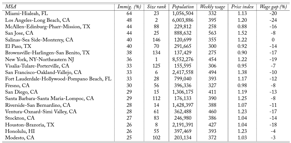
Notes: This table shows a number of statistics for the sample of metropolitan statistical areas with the highest immigrant shares. These statistics are based on the sample of prime-age workers (25-59) from the 2000 census. Weekly wages are computed from yearly wage income and weeks worked. Local price indices are computed following Moretti (2013). The wage gap is the gap in wage earnings between natives and immigrants (a negative number means that natives’ wages are higher), controlling for observable characteristics.
The second data set that we use is the Consumer Expenditure Survey, which is maintained by the Bureau of Labor Statistics and has been widely employed to document consumption behavior in the United States. It is a representative sample of US households and contains detailed information on consumption expenditure and household characteristics. Unfortunately, it contains no information on birthplace or citizen status, which is why it is impossible to directly identify immigrants. Instead, we rely on one of the Hispanic categories that identifies households of Mexican origin in the years 2003 to 2015.12Monras (2015b) shows that the overlap between individuals identified as Hispanics of Mexican origin and Mexican-born individuals is around 85 percent in census data. This gives us confidence that, by using the Hispanic variable in Consumption Expenditure data, we are capturing a large number of Mexican-born individuals. The data set contains around 30,000 households per year, of which around 7 percent are of Mexican origin.
2.3 Real exchange rate data
The World Bank provides real exchange rates with respect to the United States for a large number of countries in its International Comparison Program database.13The exact title of the series is “Price level ratio of PPP conversion factor (GDP) to market exchange rate.” These data expand the 89 countries of origin that we use in our estimation exercise.14An alternative source of similar information is provided by the OECD and the Penn World Tables. The OECD also estimates price levels of various countries. The number of countries that the OECD covers is smaller, which is why we report estimates in the paper using the World Bank data, although estimates for OECD countries may be more reliable because they cover richer, more developed, countries. We obtain similar estimates using OECD data. We also obtain similar estimates using the GDP per capita in the country of origin, obtained from the Penn World Tables, to proxy for the price index. In table 2, we provide a list of the top and bottom 10 countries in terms of the average real exchange rate with respect to the United States over the years 1990, 2000, 2010. Prices in countries like Norway and Japan are around 35 percent higher than in the United States. However, there are not many countries in the world where prices are higher than in the United States. Australia, ranked 10th in the table, is only 7 percent more expensive than the United States. On the other end, prices in countries like Vietnam (with large immigrant communities in the United States) have prices that are only 20 percent of those in the United States.
Table 2. Countries with the highest and the lowest real exchange rates
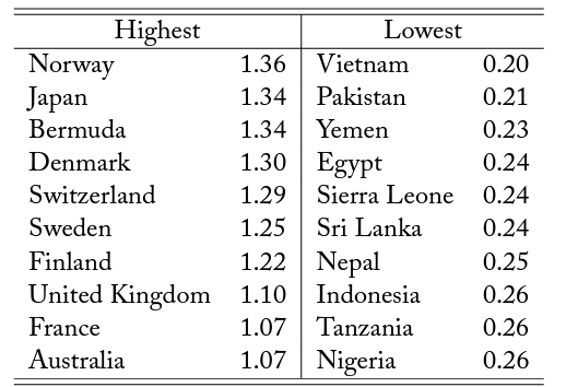
Notes: This table lists the top and bottom 10 countries with the highest and the lowest average real exchange rate with respect to the United States according to real exchange rate data from the World Bank from the years 1990, 2000 and 2010.
3 Empirical evidence
In this section, we start by documenting a series of facts about immigrants’ location choices and wages. In particular, we show that immigrants concentrate much more than natives in large, expensive cities and that they tend to earn less than natives there. We also demonstrate that these patterns are stronger for immigrants coming from countries with lower price levels, as measured by the real exchange rate, and for Mexicans who moved to or within the United States in years with low real exchange rates. We then show that Mexicans from poorer origin states in Mexico disproportionately move toward richer states of destination in the United States. We also show that the patterns are stronger for immigrant groups that are likely to be less attached to the United States. We argue that these patterns are driven by the differential consumption patterns of natives and immigrants, which we document by showing that immigrants tend to consume less than similar-looking natives at the local level.
3.1 Immigrants’ location choices and city size
The first fact that we document in this paper is that immigrants tend to live in larger, more expensive cities in greater proportions than natives. This is something that was known to some extent in the literature (Eeckhout et al. 2014; Davis and Dingel 2012) but here we document it much more systematically; we use a much larger number of data sets and we expand the existing literature by showing that there is also a strong relationship between immigrant shares and local price indices.
A simple way to document this fact is to regress the distribution of immigrants relative to the distribution of natives on city size or price level. In order to do this, we define the relative immigrant share as the share of immigrants living in city c divided by the share of natives living in city c and regress this measure (in logs) on the size or price level of city c. More specifically, we run the following regression:
![\[\ln \left(\frac{\operatorname{Imm}_{c, t}}{\mathrm{Imm}_t} / \frac{\mathrm{Nat}_{c, t}}{\mathrm{Nat}_t}\right)=\alpha_t+\beta_t \ln P_{c, t}+\varepsilon_{c, t}\]](https://www.thecgo.org/wp-content/ql-cache/quicklatex.com-196e75092492fdfd9889799e2f1237e2_l3.svg "Rendered by QuickLaTeX.com")
where Imm is the number of immigrants and Nat is the number of natives in city
  at time
  . When the subscript is omitted, the variables represent the total number of immigrants or natives living in the country in a particular time period.15We only use urban population for the entire analysis. Non-urban local labor markets are usually defined by commuting zones (Autor et al. 2013). To define non-urban commuting zones we need information on county of residence, which is not provided for ever year in CPS data. Urban commuting zones and MSAs are essentially the same.
  is either the total number of people in the city or its price level. We run separate regressions for each year.
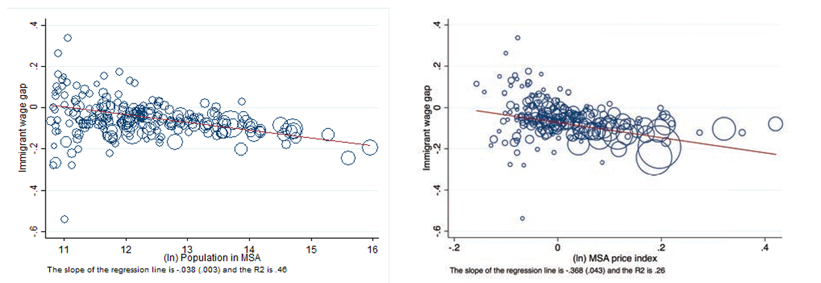
Figure 1 shows these relationships using data from the 2000 census. In the left-hand panel, we observe that, even if there is some variance in the relative immigrant share across metropolitan statistical areas, there is a positive and statistically significant relationship between the distribution of immigrants and city population. The marker sizes are proportional to the respective city price indices and indicate that the more populous cities also tend to be more expensive. The relationship between the relative immigrant share and price indices shown in the right-hand panel is even stronger, and the linear fit is better.16This is also the case when we include both city price and city size in a bivariate regression. Here, marker sizes reflect city population levels. While there are some outliers, mainly along the US-Mexico border, a city with a local price index that is 1 percent higher is associated with an 8 percent higher relative immigrant share. In appendix A.3, we show that this relationship also holds when using commuting zones instead of MSAs.17Commuting zones are a partition of the US territory. Commuting zones can be divided between urban and rural commuting zones. Urban commuting zones are equivalent to MSAs, whereas rural commuting zones are not captured by MSA information. This evidence is in line with the contemporaneous paper by Albouy et al. (2018), which argues that immigrants live in relatively high-nominal wage, low-amenity locations.
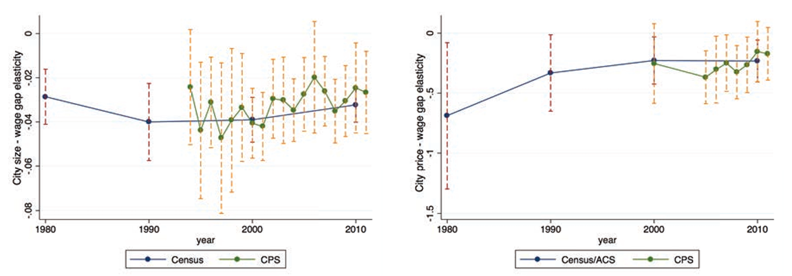
In figure 2, we investigate how these relationships have evolved over time. To show this, we first run a linear regression following equation 3.1 for each of the years displayed along the x-axis of the figure against the city size or the price index, and we then plot the various estimates and confidence intervals for these elasticities.
Figure 1. City size, price index, and relative immigrant share
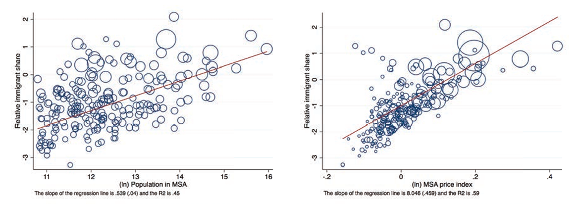
Notes: This figure shows the relationship between the relative share of immigrants in an MSA and the MSA population (left) and price index (right). The relative share of immigrants is measured as the number of immigrants in the MSA relative to all immigrants in the United States divided by the number of natives in the MSA relative to all natives in the United States. The figure is based on the sample of prime-age workers (25-59) from the 2000 census. The MSA price indices are computed following Moretti (2013). Each dot represents one of 219 MSAs in the sample. Marker sizes reflect MSA price indices in the left-hand plot and population level in the right-hand plot.
Figure 2. Evolution of the city size/price elasticity of the relative immigrant share
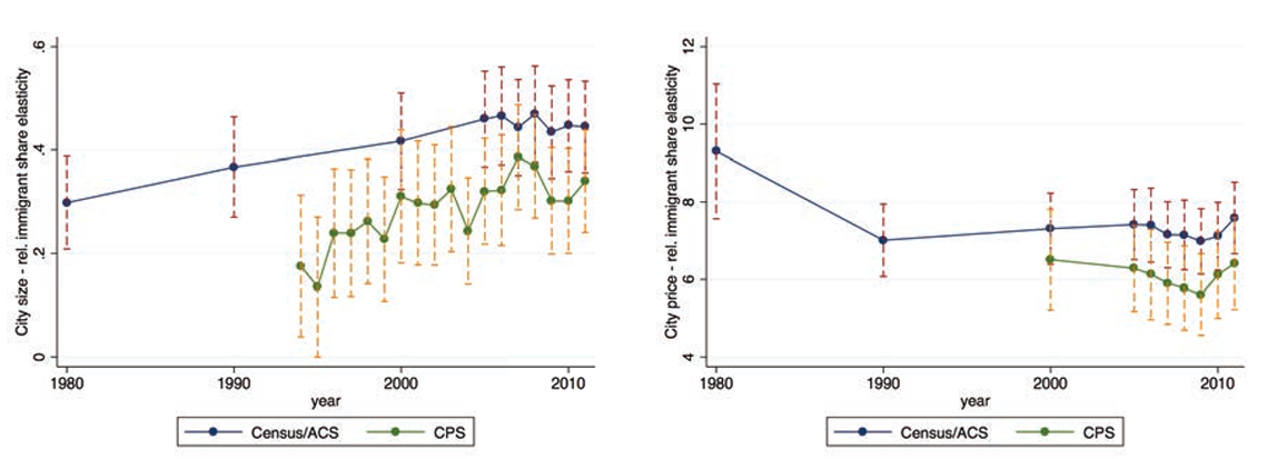
Notes: Each dot in this figure shows the cross-MSA elasticity between the relative share of immigrants in an MSA and the MSA population (left) and the price index (right), for each year indicated in the x-axis. The relative share of immigrants is measured as the number of immigrants in the MSA relative to all immigrants in the United States divided by the number of natives in the MSA relative to all natives in the United States. Vertical lines represent 95% confidence intervals. This figure uses census, ACS, and CPS data from 1980 to 2011. Price indices are computed following Moretti (2013) and can only be computed when census and ACS data are available.
The left-hand panel in figure 2 shows that the relationship between the relative immigrant share and city size has been positive since the 1980s and has become slightly stronger over time. While in 1980 the elasticity was around 0.3 percent, it has increased over the years to reach almost 0.5 percent when using the census data. We observe a similar trend in the CPS data, but estimates are smaller and noisier, driven by measurement error of city sizes. The elasticity of immigrant shares and local price indices first decreased from around 9 to 7 percent between 1980 and 1990 but has remained relatively stable since then.
3.2 Native – Immigrant wage gaps
In this subsection, we investigate how the gap in (composition-adjusted) wages between natives and immigrants is related to city size and city prices. If wages reflect, at least in part, the value of living in a location – which is a natural result in non-competitive labor market models, see section 5 – we should expect the relationship between wage gaps and city size and city prices to be the mirror image of relative location choices documented in section 3.1. To investigate this, we run Mincerian type regressions of the following type:
![\[\ln w_{i, c, t}=\alpha_{1 t}+\alpha_2 \operatorname{Imm}_{i, c, t}+\beta \operatorname{Imm}_{i, c, t} * \ln P_{c, t}+\gamma \ln P_{c, t}+\phi X_{i, c, t}+\varepsilon_{i, c, t}\]](https://www.thecgo.org/wp-content/ql-cache/quicklatex.com-4d57d9c2797b2b19fa2a3aed7899a4f2_l3.svg "Rendered by QuickLaTeX.com")
where  indexes individuals, indexes cities, indexes years,
  is an indicator variable for being an immigrant, ln
  indicates city size or city prices, and
  contains observable individual characteristics.18The individual controls are five dummies for race (white, black, American Indian/Aleut/Eskimo, Asian/Pacific Islander, other), five for marital status (married, separated, divorced, widowed, never married/single), four age groups (three 10-year intervals from 25 to 54 and 55 to 59), four education categories (high school dropout, high school graduate, some college, college graduate or more), and 82 occupation categories, which are based on the grouping of the 1990 occupation codes from https://usa.ipums.org/usa/volii/occ1990.shtml. An estimate of β < 0 means that the gap in wages between natives and immigrants is larger in large or more expensive cities.19We also obtain β < 0 when including year and MSA fixed effects using multiple years of data. See, for example, table 4. Note that these regressions can also be used to compute city-specific wage gaps and immigrant-native wage gaps, which are useful for visualizing the estimate of β. In the results that we report in the main text, we do not interact the controls
  with the immigrant dummy. Not doing so assumes that the returns to observable characteristics are the same between natives and immigrants, which is what we later implicitly assume in the model. In table A.1, discussed in appendix A.1, we show that the results do not change if we interact the controls with an immigrant dummy.
As before, we present the results in two steps. Figure 3 shows the estimates using data from the 2000 census. In the left-hand panel, we plot the difference in composition-adjusted wages between natives and immigrants in our sample of metropolitan statistical areas against the size of these cities.20We generate these wage gaps at the city level by running a regression similar to 3.2 but interacting the immigrant dummy with MSA dummies instead of population and taking the coefficients of these interactions as city-specific wage gaps. The relationship is negative and strong. The estimate is -0.038, meaning that if a city is 10 percent larger, the gap in wages between natives and immigrants is 0.38 percent larger. Moreover, the relationship between native-immigrant wage gaps and city size is very tight. The R squared is around 0.46, and the standard errors of the estimate are small. In appendix A.3, we show that this result also holds when using commuting zones instead of MSAs. The results also hold when we exclude Mexicans – which is the main immigrant group in the US – from the wage regressions, as can be seen in table A.1 in the appendix.
One way to assess the stability of the relationship between native-immigrant wage gaps and city size over
Figure 3. City size, price index, and wage gaps
Notes: This figure plots the relationship between the gap in wages between immigrants and natives (controlling for observable characteristics) and the metropolitan statistical area (MSA) population and price index. A negative number for the native-immigrant wage gap means that immigrants are paid less than natives in that MSA. The figure is based on the sample of prime-age male workers (25-59) from the 2000 census. The MSA price indices are computed following Moretti (2013). Each dot represents one of 219 MSAs in the sample. Marker sizes reflect MSA price indices in the left-hand plot and population level in the right-hand plot.
time is estimating the model for each year. The results are shown in figure 4. As before, we show the estimates using both census and CPS data over a number of years between 1980 and 2011. The relationship remains tight at around 0.035 through the entire period in both data sets. The right-hand panels of figures 3 and 4 show the relationship between native-immigrant wage gaps and local price levels. We also observe a negative and tight negative relationship. If anything, it seems that over time, this relationship has become a little weaker but remains at around -0.36.
To the best of our knowledge, this is the first paper to document this very strong feature of the data in the United States. It suggests that, for whatever reason, immigrants who live in larger, more expensive cities are paid less (relative to natives) than immigrants who live in smaller, less expensive cities.21On average, immigrants earn less than natives, but this is driven mostly by immigrant wages from lower-income countries and by immigrants of all income levels in larger cities. This is not driven by the composition of immigrants across US cities. In figures 3 and 4, we control for observable characteristics, which include education, race, marital status, occupation, and so forth. Furthermore, we check that this relationship prevails for each education group independently by running separate regressions by education category, and we check that it is robust to controlling for immigrant networks, imperfect native-immigrant substitutability, and legal status, as reported in appendix A.1. We discuss this in more detail in section 3.5.
Figure 4. Evolution of the city size/price elasticity of the wage gap
Notes: Each dot in this figure shows the cross-MSA elasticity between the relative gap in wages between immigrants and natives (controlling for observable characteristics) in a metropolitan statistical area and the MSA population (left) and price index (right) for each year indicated in the x-axis. This figure uses census, ACS, and CPS data from 1980 to 2011. Price indices are computed following Moretti (2013) and can only be computed when census and ACS data are available.
3.3 Immigrant Heterogeneity
3.3.1 Heterogeneity by real exchange rate
In section 5 below, we argue that the results reported so far can be explained by the fact that part of what immigrants consume is related to the home country. This implies that if there is some degree of substitution between consuming locally or consuming in the country of origin, the patterns documented so far should be stronger for immigrants coming from countries of origin with lower price levels relative to the United States or, in other words, lower real exchange rates with respect to the US dollar.
To show that this is indeed the case, we perform two alternative exercises in this subsection. First, we show that the relationships between local price indices and both location choices and wage gaps are stronger for immigrants from countries with lower real exchange rates. We use both across and within-country variation to document this fact. Second, we use exchange rate fluctuations between Mexico and the United States to show that these patterns are stronger for Mexicans that migrate to the United States when the real exchange rate of the Mexican peso is low.
Before using a regression framework, we first show in a simple graph the elasticities of relative locations and wage gaps of immigrants from different countries of origin as a function of the real exchange rate for the year 2000. For this, we estimate equation 3.1 at the city-origin level (i.e., we replace by the immigrant population from the respective origin, and we estimate β for each origin). We then estimate the same specification with the wage gaps as dependent variable, which are calculated for each city as the difference in natives’ and immigrants’ mean residual obtained from a regression of the wage on the control vector (see equation 3.2).
One challenge of this exercise is that there are some countries of origin for which we observe immigrants only in a subset of the MSAs of our sample, and hence there are some zeros when computing relative immigrant shares at the MA-origin level. To address this, we concentrate on the top 100 MSAs by size and the top 89 sending countries.22Different selections of MSAs lead to slightly different selections on the number of sending countries, which results in small changes in the estimates. Expanding the number of MSAs tends to introduce more measurement error, which attenuates the estimates of the regressions with many fixed effects. Reducing the number of MSAs obviously reduces the number of observations, which has small consequences on the point estimates and confidence intervals.Figure 5 shows the plots of the city price elasticities and city size elasticities of the relative immigrant share against real exchange rates in panel A and the elasticities of the wage gap in panel B. All plots show statistically significant relationships that go in the expected direction. Panel A shows that the elasticity of the relative share of immigrants with respect to city size or city price from countries with lower real exchange rates is higher. This means that immigrants from low price index countries concentrate more in bigger and more expensive cities than immigrants from richer countries of origin. The relationship of the elasticity of the wage gap with respect to city size or city price and real exchange rates is the mirror image of the relative location choices.23Recall that the wage gap is defined as immigrant wage minus native wage. Therefore, a negative elasticity indicates an increasing wage gap. As can be seen in panel B, the elasticity of the wage gap is higher for immigrants from higher price indices, meaning that the difference in wages between natives and immigrants does not increase as much for immigrants from high price, richer countries of origin. Overall, these graphs show that there is substantial variation across countries of origin, which is well aligned with the role that differences in prices should play in shaping the importance of home country expenditures for immigrants from different countries of origin.24An alternative to this exercise is to see if the interaction of the immigrant dummy and city size or city price of equation 3.2 is higher at lower quantiles of the wage distribution. We show that this is indeed the case in figure A.1 of the appendix.
To document these relationships more systematically, we expand equations 3.1 and 3.2 by interacting the city variable directly with the real exchange rate (RER) and use data not just for 2000 but for all our available censuses also. In particular, we estimate regressions of the following type:
![\[\begin{aligned} & \ln \left(\frac{\operatorname{Imm}_{c, o, t}}{\operatorname{Imm}_{o, t}} / \frac{\mathrm{Nat}_{c, t}}{\mathrm{Nat}_t}\right)=\alpha_1 \ln P_{c, t}+\alpha_2 \ln R E R_{o, t}+\alpha_3 \ln P_{c, t} * \ln R E R_{o, t}+\delta_t+\left(\delta_o+\delta_c\right)+\varepsilon_{c, t} \\ & \quad \ln w_{i, c, t}=\beta_1 \ln P_{c, t}+\beta_2 \ln R E R_{o, t}+\beta_3 \ln P_{c, t} * \ln R E R_{o, t}+\delta_t+\left(\delta_o+\delta_c\right)+\phi X_{i, c, t}+\varepsilon_{i, c, t} \end{aligned}\]](https://www.thecgo.org/wp-content/ql-cache/quicklatex.com-545e933f93726e5ab9051323e9c861dc_l3.svg "Rendered by QuickLaTeX.com")
where as before ln denotes the population or the price level of MSA , and  is the real exchange rate of origin country
  with respect to the United States.
  and
and  are country of origin and year fixed effects, respectively. We estimate the relative share equation using a PPML regression model in order to deal with the incidence of zeros (Santos Silva and Tenreyro 2006). The wage regressions are simply extended Mincerian type regressions like the ones we used before, since
  is zero for individuals born in the United States and a continuous variable instead of the immigrant dummy.
Figure 5. City size/price elasticity of relative immigrant share and wage gap by origin price level
Panel A: Relative immigrant shares
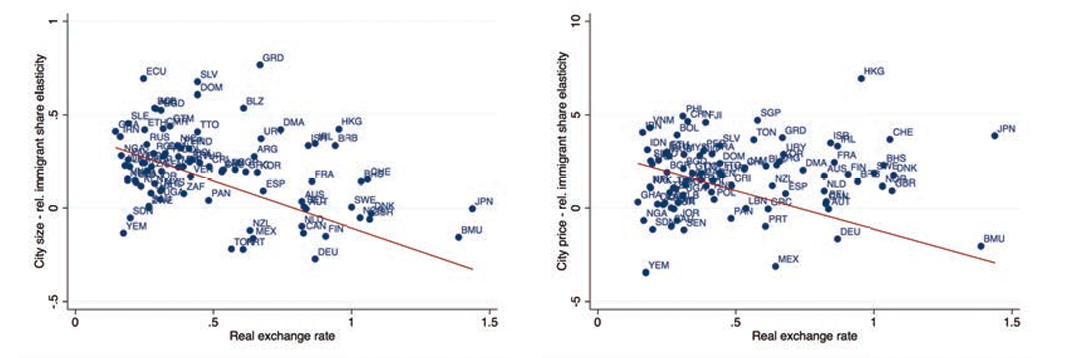
Panel B: Wage gap elasticities
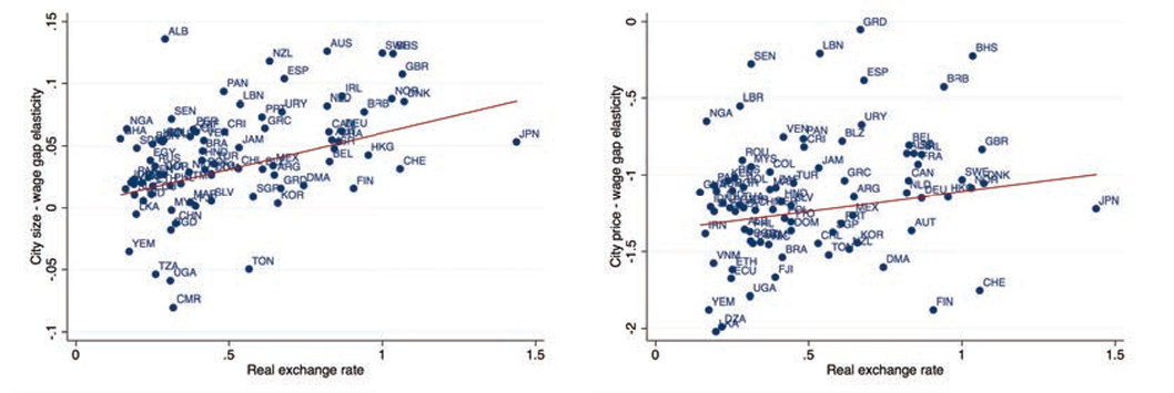
Notes: This figure uses data from the 2000 census to show the elasticity between the relative immigrant shares (panel A) and the native-immigrant wage gaps (panel B) and the city size and city price, for each of the different countries of origin, as a function of the country of origin price level. Hence, each dot represents an estimate of the coefficient β in equation 3.1 and equation 3.2, restricted to each country of origin.
The estimates of interest are  and
and  . A negative estimate of means that immigrants from cheaper countries tend to concentrate more in larger, more expensive cities. Similarly, a positive estimate of
  and ), the identifying variation comes from RER fluctuations across decades for each country of origin. When not including the fixed effects, the identifying variation comes from comparison across country of origin.
We present the results on relative immigrant shares in table 3. In the first column, we only include the real exchange rate. A positive estimate means that the distribution of immigrants from countries of origin with higher exchange rates tends to be more similar to the distribution of natives. This is because the relative immigrant share is on average higher if the distributions of immigrants and natives are more similar. The relationship is not very strong, however. In the second column, we include the population. This replicates
Table 3. Immigrant heterogeneity: location choices
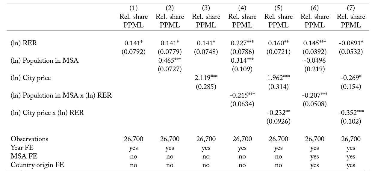
Notes: This table shows regressions of relative immigrant shares and wages on population and city prices, real exchange rates (RER), and their interaction. The regressions are limited to the top 100 MSAs in size and 89 sending countries for the years 1990, 2000, and 2010. Standard errors clustered at the MSA-country of origin level are reported. We weight each observation by the number of individuals in a year-MSA-origin cell. * significant at the 0.10 level; ** significant at the 0.05 level; *** significant at the 0.01 level.
the result we showed before. The relative share of immigrants is increasing in city size and city price, as shown in column 3. In column 4, we introduce the interaction between real exchange rates and city sizes. A negative estimate suggests that the relative concentration of immigrants from high exchange rate locations (e.g., Japan, Germany, or the United Kingdom) in larger cities is less strong than for immigrants from lower price indices (e.g. India or China). Column 5 repeats the specification of column 4 but uses city prices instead of city sizes. The estimate is, again, negative, suggesting that immigrants from low price index countries disproportionately locate in larger and expensive cities. The identifying variation in columns 4 and 5 comes from comparing different countries of origin. In columns 6 and 7, which are our preferred specifications, we include country of origin and location fixed effects. This means that we compare the relative location of immigrants within each country of origin as a function of exchange rate fluctuations.
The estimates using this variation are quite similar in magnitude to the ones using cross-origin variation.
Table 4 repeats the exercise for wages. Table 4 shows that relative wages of immigrants are essentially the mirror image of relative location choices. In column 1, we include the real exchange rate in an otherwise Mincerian regression. This shows that immigrants from high price index countries tend to have higher wages than the ones from low price index countries. This likely reflects a combination of the unobservable skills brought to the United States and the outside option in the wage determination process. In the second column we include the size of the location, and in the third column we include city prices. As it is well known, larger and more expensive cities tend to pay higher wages, both to immigrants and to natives. In column 4 we include the interaction between city size and country of origin real exchange rate. A positive coefficient means that for countries of origin with high price indices, the city price premium increases more than for lower price countries of origin, and similarly, with city prices, as shown in column 5. Columns 6 and 7 repeat the exercise controlling for country of origin and location fixed effects (i.e., using within-origin variation). The results are, in what is our preferred specification, quite similar to those in columns 4 and 5.
Table 4. Immigrant heterogeneity: wage gaps
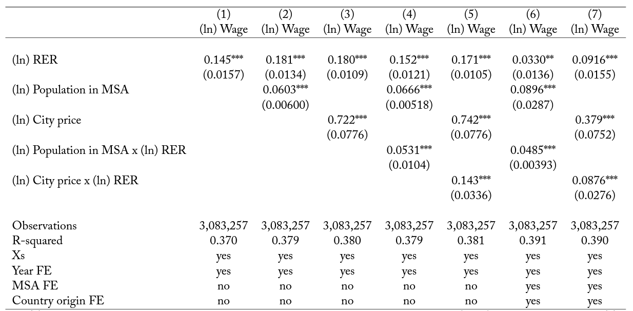
Notes: This table shows regressions of wages on population and city prices, real exchange rates (RER), and their interaction. The (ln) real exchange rate for natives is equal to 0; hence, the interaction between the real exchange rate and MSA population size or price level is the differential slope in wages between natives and immigrants as a function of the real exchange rate. The regressions are limited to the top 100 MSAs in size and 89 sending countries for the years 1990, 2000, and 2010. Standard errors clustered at the MSA-country of origin level are reported. * significant at the 0.10 level; ** significant at the 0.05 level; *** significant at the 0.01 level.
One caveat of the results shown in tables 3 and 4 is that we can only use exchange rate variation over the 10-year gaps when census data is available. To complement this evidence we also use higher frequency fluctuations in real exchange rates. Exchange rate fluctuations are common and difficult to anticipate over short time horizons.25In this paper, we complement the evidence shown in Nekoei (2013). Exchange rate fluctuations affect not only the intensive margin of immigrant labor supply decisions (i.e., hours worked) but also, and very importantly, the extensive margin (i.e., location choices). More concretely, we use variation in the exchange rate between the United States and Mexico for each year and focus our analysis on Mexican immigrants who move to the United States from abroad or who move within the United States across states in a given year. We investigate whether these immigrant movers concentrate more in large cities in years when prices in their home country are lower. For this exercise, we use the yearly CPS data and concentrate on Mexican migrants, as they are by far the largest immigrant group, and thus measurement error is smaller. We can only compute city size
Figure 6. City size elasticity of relative immigrant share and wage gap of Mexicans
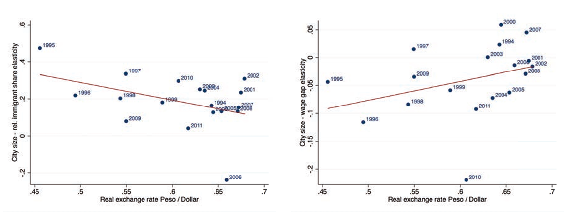
Notes: This figure uses data from the CPS 1994-2011 to show the relationships between the relative immigrant share and the (composition-adjusted) wage gap of Mexican immigrants who changed location during the indicated year and the city size elasticity. More specifically, we estimate the elasticity for each year and plot it against the average real exchange rate of the Mexican peso to the US dollar during that year. Hence, each dot represents an estimate of the coefficient β for the particular year based on equations 3.1 and 3.2. We can only compute city size elasticities because price indices can only be computed using ACS and census data, which is available only in selected years. elasticities because CPS data does not include the necessary information to compute city price levels as in Moretti (2013).
As before, we estimate equations 3.1 and 3.2 using Mexican movers separately for each year and plot the β coefficients against the average real exchange rate of the Mexican peso to the US dollar during that year.26We do not take the log of the left-hand side of equation 3.1 to avoid losing MSAs without Mexican immigrant movers. The two plots in figure 6 show a linear fit that goes in the expected direction. The lower the prices in Mexico are relative to US prices, the more positive is the elasticity of the relative share of Mexican immigrants and the more negative the elasticity of the wage gap with respect to city size.
3.3.2 Heterogeneity by state of origin in Mexico
To explore immigrant heterogeneity even further, in this subsection we use data on Mexican flows from particular states of origin in Mexico to particular states of destination in the United States.27The publicly available Matricula Consular data is only available at the state level. What we have argued would suggest that immigrants from low price index origins in Mexico would disproportionately move to high price index destinations in the United States.
Unfortunately, we do not have local price index data for Mexican locations. Instead we use GDP per capita at the state level to proxy for local price indices. There is usually a strong correlation between price levels, wages levels, and GDP per capita, which suggests that using GDP per capita is a good proxy.
To investigate the heterogeneity in migration flows by Mexican state of origin we use the following estimation equation:
![\[F_{i j}=\beta_1 \ln P_i+\beta_2 \ln P_j+\beta_3 \ln P_i * \ln P_j+\left(\delta_i+\delta_j\right)+\varepsilon_{i j}\]](https://www.thecgo.org/wp-content/ql-cache/quicklatex.com-f8e5a0672f6df5d77fd1e75fd0fb9bbe_l3.svg "Rendered by QuickLaTeX.com")
where  is either the fraction of all immigrants from origin that move to destination
  or the log of this fraction,
  is the GDP per capita in , and
  is the GDP per capita in . In some specifications we also control for the level of population at origin and destination, or by origin and destination fixed effects. Our main hypothesis is that is negative. If
  it means that there are relatively less flows to high GDP pc destinations from higher GDP pc origin states.
Table 5. Mexican Immigrant Flows
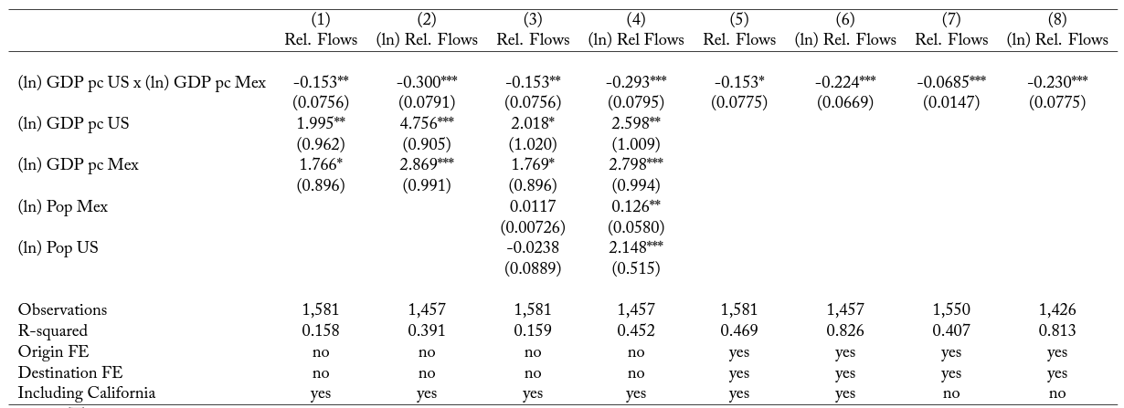
Notes: This table shows the results of regressing the flows of immigrants from origin to destination j relative to all migrants from Mexican state i on the GDP per capita at destination (j), at origin (i), and the interaction between the two. We also control for total population at origin and destination. The data covers 31 sending Mexican states and 51 receiving US states. Columns (7) and (8) exclude the largest destination state (California) from the regression. Data from the Matricula Consular 2016. Robust standard errors clustered at the destination level are reported. * significant at the 0.10 level; ** significant at the 0.05 level; *** significant at the 0.01 level.
Table 5 presents the results. In the first two columns we simply explain the flows of Mexican immigrants from origin to destination by the GDP per capita at origin and at destination. Mexicans of all origins tend to disproportionately move to high GDP per capita states in the United States. This can be read as further corroborating that immigrants prefer to move to high nominal income locations. The positive coefficient of origin per capita GDP shows that there are more migrants from high GDP per capita origin states. Selection or credit constraints when migrating can explain this result (Angelucci 2015). The next two columns control for the size of the origin and destination states. This is an important control since larger origin states and larger destination states likely send and receive more migrants, respectively. In the final two columns, we include state of origin and state of destination fixed effects. These should control for unobservable characteristics of the states that go beyond size and GDP per capita. The last two columns exclude California as a destination state. All the specifications show the same result. There is a disproportionate flow of immigrants from low GDP per capita origin states towards high GDP per capita destinations.
3.3.3 Heterogeneity by attachment to the United States
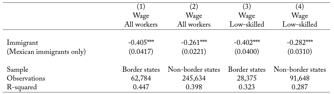
An alternative source of heterogeneity is potentially provided by Mexicans who live closer to or farther from the border. The former are likely to have stronger ties to Mexico. These ties may take various forms. When living closer to the border, it may be easier to spend longer periods of time in Mexico and to stay in closer touch with family members not in the United States; thus the weight of the home country may be greater. We can use this insight to see whether the wage gap between Mexicans and natives, and the relationship between this gap and city size, is stronger for Mexicans close to the border.28Cities close to the Mexican border are defined as locations in California, Arizona, New Mexico, or Texas, which are the four US states that share a border with Mexico. For this, we run the wage regressions with Mexican immigrants separately for people living in cities in border states and for people living in non-border states. In order to account for characteristics of Mexicans that might differ across these samples and are that likely to influence wages, we include years in the United States and a dummy for being undocumented as additional controls.
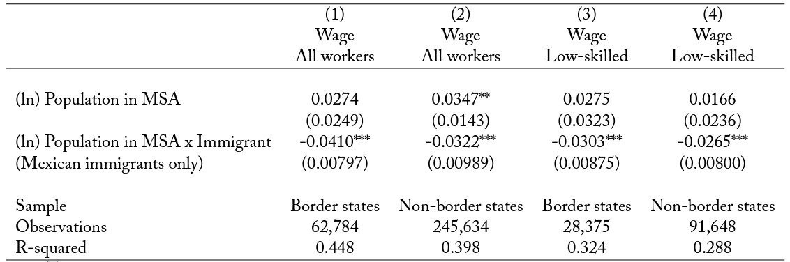
The first two columns of panel A in table 6 show that Mexicans living in border states earn less relative to natives than Mexicans in non-border states. This could suggest that the opportunity to spend a larger part of the income at lower prices across the border allows Mexicans to accept lower wages. There are also alternative explanations for these results, so it is worth emphasizing that we take them purely as suggestive evidence that the mechanism posited in this paper may be relevant for explaining these patterns in the wages of immigrants of the same country of origin. Columns 3 and 4 show that the same is true when we restrict the sample to low-skilled workers, suggesting that the differences reported in columns 1 and 2 are not driven by human capital differences. Columns 1 and 2 of panel B show that the gap in wages between Mexicans and natives decreases faster with city size in locations close to the Mexican border than in locations farther away. Thus, Mexicans earn less if they are closer to the border than they do if they are farther away. Additionally, the relationship between Mexican-native wage gaps and city size is stronger. Columns 3 and 4 of this panel restrict the regressions to low-skilled workers, again showing that the results are not driven by human capital differences.
Another variable that is potentially related to host country attachment is immigrants’ length of stay in the United States. According to Dustmann and Mestres (2010), immigrants who do not intend to return to their countries of origin remit a smaller share of their income. They are also less likely to spend time back home and thus are, in some way, more similar to natives. There is also a large body of literature starting with Chiswick (1978) that estimates the speed of assimilation into the receiving country. This literature has interpreted the early gap in wages between natives and immigrants as the lack of skills specific to the receiving country. While this is certainly a possibility, it does not explain why this gap increases with city size. However, we can use the insights from the immigrant assimilation literature to see whether the relationship between city size and city price level is stronger for newly arrived immigrants than for immigrants who have been in the United States longer. To investigate these ideas, we use the year of immigration taken from the census data and divide immigrants into groups depending on their time spent in the United States. We plot the city size-wage gap elasticities and city price-wage gap elasticities for different groups of immigrants by the years since arrival in figure 7. The positive slope in each graph of the figure indicates that the differences in wages between natives and immigrants (and how they relate to city sizes and prices) tend to diminish the longer an immigrant remains in the United States.
Table 6. Mexican – native wage gaps and distance to Mexico
Panel A
Panel B
Notes: This table reports wage regressions for different samples of Mexicans, showing the differential wage of Mexican immigrants to natives (panel A) and the wage of Mexican immigrants and how it changes with city size (panel B). These regressions only report selected coefficients. The complete set of explanatory variables is specified in equation 3.2, and is expanded by including the number of years that Mexicans have been in the United States. MSA and year fixed effects are also included in the regression. These regressions use CPS data for the years 1994 to 2011. Low-skilled workers used in columns (3) and (4) are defined as being high school graduates or less. Robust standard errors, clustered at the MSA level, are reported. * significant at the 0.10 level; ** significant at the 0.05 level; *** significant at the 0.01 level.
3.4 Immigrant consumption and return migration patterns
In this section, we document the importance of consumption in the home country by analyzing remittance behavior, housing expenditure, consumption expenditure, and return migration patterns. All our findings are in line with the notion that a part of the income (or potentially of future income) of immigrants is spent at the country of origin.
Figure 7. City size/price elasticity of wage gap by immigrants’ years in the country
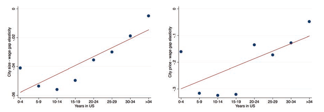
Notes: This figure uses data from the 2000 census to show the relationships between the city size and city price elasticity of the native-immigrant (composition-adjusted) wage gap as a function of the time spent in the United States, shown in the x-axis. More specifically, each dot represents an estimate of the coefficient β for the particular group based on equation 3.2.
3.4.1 Remittances
Dustmann and Mestres (2010) report that immigrants in Germany remit around 10 percent of their disposable income. While data of similar quality as in their study do not exist for the United States, we can use the New Immigrant Survey to get some notion of the remittance behavior of newly admitted immigrants in the United States. Table 7 reports the likelihood, the share of income, and the share of income for those immigrants who remit, for a number of different origins. There is quite some variation in the likelihood of remitting across origins. For example, 20 percent of immigrants from Mexico and as much as 32 percent of immigrants from other Latin American countries seem to remit part of their income to their home countries. This number is significantly lower for immigrants from European countries.
Table 7. Remittances
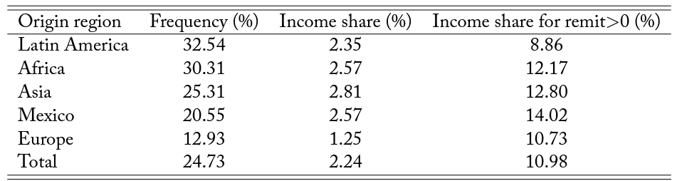
Notes: This table uses data from the 2003 New Immigrant Survey (NIS). The NIS is a representative sample of newly admitted, legal permanent residents. Statistics are based on the subsample of immigrants with positive income (from wages, self-employment, assets, or real estate) and with a close relative (parent, spouse, or child) living in the country of origin. Income shares over 200 percent are dropped.
For the entire population of immigrants, immigrant remittances represent between 2 percent and 3 percent of income, approximately. For those who remit, this number logically increases to between 10 percent and 15 percent, which is closer to the estimate provided in Dustmann and Mestres (2010). All in all, the numbers for the United States seem broadly consistent with this prior literature. The main drawback of New Immigrant Survey data is that they do not include undocumented immigrants. Including that group would likely change the numbers significantly.
3.4.2 Expenditures on housing
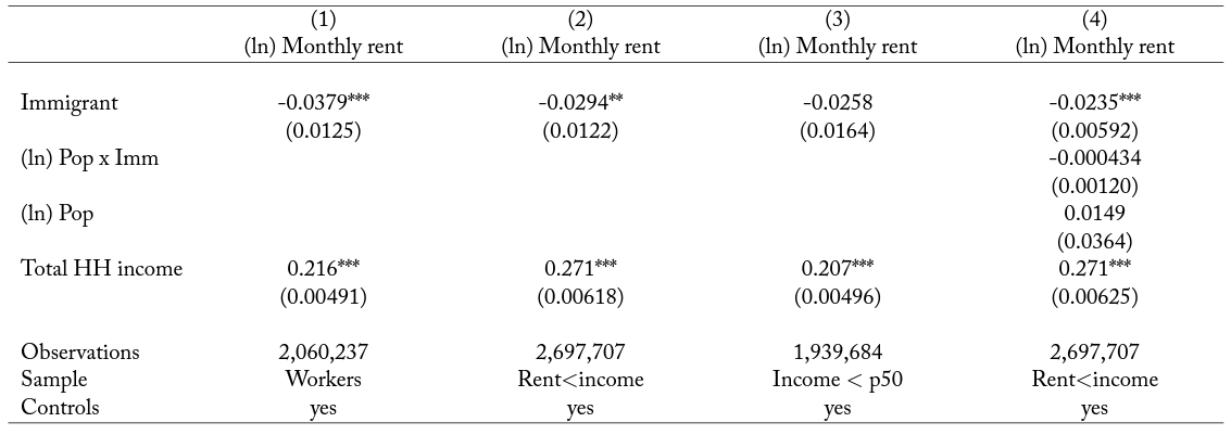
One way to explore whether immigrants consume different local goods than natives is to investigate housing expenditure. If immigrants spend a portion of their income on home goods, they should (potentially) spend less of their income on local housing (i.e., their rent).29In appendix A.4 we also show results on home-ownership status. Immigrants are less likely to own a housing unit relative to similar-looking native households. Rental prices paid vary considerably by income and other characteristics that potentially differ between the immigrant and native populations; because of this, we explore whether immigrants spend less on their rent than similar-looking natives.30In this respect, the most important controls are household income and household size. We use two alternative data sets for this. The first piece of evidence comes from census and ACS data, which can be used to compute “Monthly Rents” and total household income, and at the same time identify the country of birth of each individual. We can thus use the following regression equation to investigate whether households with at least one immigrant consume less than natives, once we control for household income and other characteristics:
![\[\text { ln Monthly Rents } i=\alpha+\beta \text { Immigrant }_i+\gamma \ln \mathrm{HH} \text { Income }_i+\eta X_i+\delta_c+\varepsilon_i \text {. }_i\]](https://www.thecgo.org/wp-content/ql-cache/quicklatex.com-e2bf24c3aab670fc216e409b08e27981_l3.svg "Rendered by QuickLaTeX.com")
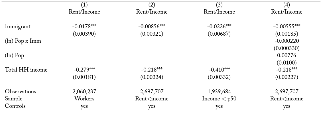
where “Immigrant” is a dummy variable indicating that household is an immigrant household, where  indicates household characteristics, and where are location fixed effects. When the (household) income measure is continuous, we can use as dependent variable “Monthly Rent/Income”, which leads to similar results, as we show below.
A different type of data that contain housing expenditure is the Consumer Expenditure Survey. The main drawback of these data is that they do not allow us to identify the country of birth of a respondent. Instead, we need to rely on the identification of Hispanics from Mexico (which should be highly correlated with Mexican-born individuals, which, in turn, is one of the main immigrant groups).31See section 2 and Monras (2015b) for a discussion of this point. In these data, moreover, we do not have a continuous measure of household income. Instead, we have nine different income categories that we include as control dummies. In particular, we run regressions of the following type:
![\[\text { ln Housing Expenditure }{ }_i=\alpha+\beta \text { Mexican }_i+\sum_j \gamma_j \text { HH Income category } j_i+\eta X_i+\delta_c+\varepsilon_i\]](https://www.thecgo.org/wp-content/ql-cache/quicklatex.com-42af86d8480361adc049b933f16fe853_l3.svg "Rendered by QuickLaTeX.com")
where “Housing expenditure” is the reported expenditure on housing and “Mexican” identifies households of Mexican origin. Note that this “Mexican” dummy identifies Mexican households with error. This means that we will likely obtain a downward biased estimate of β when using Consumption Expenditure Survey data.
The results are reported in panels A, B, and C in table 8. In panel A, we show that immigrants pay on average around 3 to 4 percent less in rental prices than comparable natives. In column 1, we use the full sample of households where the head is working and find that, once we control for personal characteristics and household income, immigrant households pay monthly rents that are around 3 to 4 percent lower compared to native households. The estimates are similar when we use all households in the sample or only the ones in the bottom half of the income distribution. In column 4, we investigate whether these results vary with the size of the city, which does not appear to be the case.32Note that a positive estimate of the interaction term between city size and the immigrant household dummy could invalidate the fact that immigrants consume less than natives in at least some locations. Panel B reports the exact same results but uses house expenditure as a share of income instead of (log) total housing expenditure as a dependent variable. The results are in line with panel A. Immigrant households consume around 1 to 2 percentage points less of their income on rents than similar-looking natives.
Panel C reports the results using Consumer Expenditure Survey data. These data do not identify metropolitan statistical area (MSA), so all comparisons are within state. In column 1, we show the regression of housing expenditure on a dummy indicating whether the household is of Mexican origin. The unconditional regression shows that it is indeed the case that these households consume less on housing. This, however, could simply reflect that they tend to earn less, or that their observable characteristics (e.g., education or residential choices) are such that these types of household tend, on average, to consume less on housing. Column 2 controls for household income. This drops the estimate to a statistical zero. Column 3 shows that controlling for personal characteristics and for time and state fixed effects is important. Mexican households tend to be systematically different than native households in terms of education, residential choices, marital status, and, most importantly, family size. When in column 4 we control for both income and personal characteristics, we see that Mexican households consume less on housing than similar-looking native households, although the difference is not as large as the unconditional regression. This is our preferred estimate and aligns well with the census estimates. Given that we do observe the MSA of residence, we cannot see whether households in larger MSAs appear to consume differently in this data set.
Table 8. Immigrants’ expenditure on housing
Panel A: Census and ACS data
Panel B: Census and ACS data, shares
Panel C: Consumer Expenditure Survey data
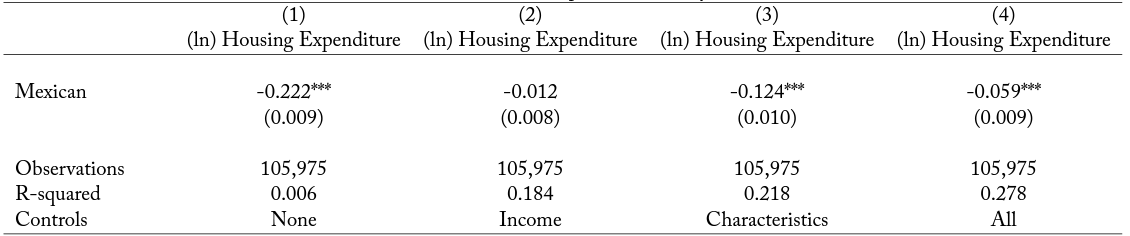
Notes: Panel A shows regressions of (ln) monthly gross rents on an immigrant dummy, (ln) total household income, and observable characteristics (including race, occupation, MSA of residence fixed effects, year fixed effects, family size, and marital status). Panel B reports regressions of the share of income spent on monthly rents on the same controls. Panel C shows regressions of (ln) housing expenditure on an immigrant dummy identifying immigrants of Mexican origin, observable characteristics (including race, occupation, state of residence fixed effects, year fixed effects, family size, and marital status), and household income bins’ fixed effects instead of a continuous measure of income. The data for panels A and B are taken from the US census and ACS from 1980 to 2011. The data for panel C are taken from the Consumer Expenditure Survey. Sample “all” uses all possible observations. Sample “workers” uses the observations where the head of the household is working. Sample “rent<income” restricts the sample to households whose total income is larger than the total rent (i.e., 12 times the monthly rent). Sample “income < p50” restricts the sample to workers in the bottom half of the earnings distribution (including homeowners and renters). Standard errors are clustered at the MSA level in panels A and B and at the state level in panel C. * significant at the 0.10 level; ** significant at the 0.05 level; *** significant at the 0.01 level.
3.4.3 Total expenditure
While it seems clear that immigrants spend less on housing than natives, it may be that they use this income on some other local goods, or rather that they save it for future consumption. To explore this, we can use the Consumer Expenditure Survey data and compare total local expenditure by Mexican households to that of all other households, following panel C in table 8.33For this section we use the variable “totexpcq” from the Consumer Expenditure Survey. This variable combines expenditures on all items. More specifically, we can use the following specification:
![\[\text { In Total Expenditure }{ }_i=\alpha+\beta \text { Mexican }_i+\sum_j \gamma_j \text { HH Yearly Income category } j_i+\eta_c X_i+\varepsilon_i\]](https://www.thecgo.org/wp-content/ql-cache/quicklatex.com-03f34b09697e274e7e851bbdd232cb06_l3.svg "Rendered by QuickLaTeX.com")
where “Total Expenditure” is quarterly total expenditure at the household level.
Table 9. Immigrants’ total expenditure, Consumer Expenditure Survey
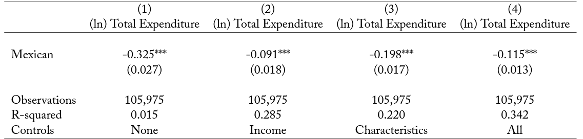
Notes: This table shows regressions of (ln) total expenditure on a number of personal characteristics (including race, occupation, state of residence fixed effects, year fixed effects, family size, marital status, household income bins’ fixed effects instead of a continuous measure of income, and an indicator identifying households of Mexican origin). Standard errors clustered at the state level. * significant at the 0.10 level; ** significant at the 0.05 level; *** significant at the 0.01 level.
The results are reported in table 9. Mimicking the results of panel C in table 8, we show that, unconditionally, Mexicans seem to consume around 32 percent less than other households. When controlling for both income and characteristics in column 4, we find that Mexican households consume around 12 percent less than other households. Given that in Consumption Expenditure Survey data we identify Mexican immigrants imperfectly (see section 2 for more details), we expect some attenuation in this estimate. This estimate is consistent with the remittances sent to their home countries or with them saving more for future consumption. We investigate whether future consumption in the home country is a potentially important channel in the following section.
3.4.4 Return migration
A final and very important reason why immigrants care about price indices in their home country is that many of them likely plan to return home at some point during their lifetime (Dustmann and Gorlach 2016; Lessem Forthcoming; Dustmann and Weiss 2007; Dustmann 2003, 1997).
To the best of our knowledge, there are no large, representative data sets directly documenting return migration patterns. This would require observations in both the destination country and the home country over a certain period of time. While there are some data sets that make this possible, they are generally not very comprehensive.
To obtain a better sense of general return migration patterns in the United States, we turn to census data. In particular, we can track the size of cohorts of immigrants and natives across censuses and use information on immigrants’ year of arrival to see how many of them are “missing” in the following census, and thus likely to have returned to their home countries.
The left-hand graph in figure 8 plots these survival rates by age cohort. We observe that more than 98 percent of the natives aged between 25 and 30 in 2000 are still present in the 2010 ACS. This survival rate declines with age. For example, for the population that in 2000 was between 45 and 50 years old, the survival rate decreases to around 94 percent. When we carry out the same exercise for immigrants who arrived in the United States before 2000, the survival rates decline substantially with respect to natives.34We use the years 2000 and 2010 because there are strong reasons to suspect that there is some undercount of immigrants in censuses prior to 2000. For example, the number of Mexican immigrants who claim to have arrived before 1990 in the 2000 census is larger than the total number of Mexicans observed in the 1990 census. See also Hanson (2006).
Figure 8. Return migration
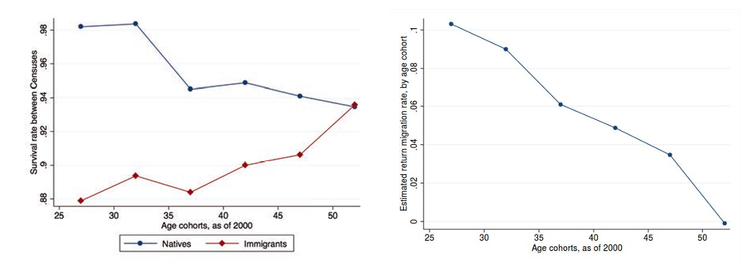
Notes: This figure shows estimates of survival rates and return migration rates by age group. The graph on the left compares the size of the cohort of natives and immigrants who arrived before 2000 in census years 2000 and ACS 2010. The difference between 2010 and 2000 in the size of the cohorts divided by the initial size of the cohort is an estimate of the cohort survival rate. The graph on the right subtracts the native survival rates from immigrant survival rates to obtain estimates of return migration rates by age group.
In the graph on the right-hand side, we estimate return migration rates by taking the difference in survival rates between immigrants and natives. This is a good estimate if mortality rates for the same age cohort are similar in both immigrants and natives. We observe that return migration is likely to be very high for younger cohorts and converges to 0 for older cohorts, perhaps reflecting that as immigrants grow old in the host country, their ties to the home country gradually diminish. The estimates show that more than 10 percent of the immigrant population aged between 25 and 30 in 2000 are no longer in the United States by 2010. We begin the series at age 25, since these immigrants are already likely to be working in the United States. Return migration rates are even higher for younger cohorts.
This means that for a large number of immigrants, future consumption takes place in a country other than the United States – possibly their home country. Thus, given that immigrants are likely to return and to care about future consumption, return migration patterns give additional support to the idea that immigrants partly take into account the price index in their country of origin when choosing their optimal location in the United States.
3.5 Discussion of alternative mechanisms
Some of the evidence presented can in principle be explained with alternative mechanisms. In this section we argue that none of the alternatives can fully explain the patterns in the data. Very often, alternative mechanisms have a hard time explaining the heterogeneity across immigrant groups. In other occasions we can explicitly control for the role of these alternative mechanisms. We discuss them in what follows and provide extra empirical evidence in appendix A.1.
There is a large literature documenting the role of immigrant networks in shaping immigrant locations (Altonji and Card 1991; Munshi 2003), so immigrant networks might be a potential explanation for some of the empirical patterns we described in previous sections. Perhaps immigrants initially settled in random locations. These locations may have grown due to subsequent immigration inflows, as predicted by immigrant networks. This could, moreover, generate bigger gaps in wages between natives and immigrants in these cities if newer immigrant inflows put disproportionate pressure on wages of immigrants.
To address this concern, we extend our wage gap regressions with a control for the relative size of the immigrant community within the MSA for each of our countries of origin. As shown and discussed in more detail in the appendix A.1, table A.2, including immigrant networks as a control does not change our main results. Furthermore, it is difficult to explain the country of origin immigrant heterogeneity. It is unclear why immigrants from low-income countries would concentrate in large and expensive cities in the earlier periods, or why cities where immigrants from low-income countries concentrate grow disproportionately more than cities with more immigrants from higher-income countries. In general, the evolution of city sizes is slow and the level of immigration in the United States not sufficiently large to dramatically change city size rankings (Duranton 2007). In appendix A.1, see table A.1, we show that our results do not change if we measure city size using only native population or using lagged city size. Neither do they change if we exclude the largest immigrant group (Mexicans) in the wage regressions.
Taken altogether, we think that it is more likely that immigrants keep going to the same large and expensive cities not just because former immigrants moved into them, but because the same incentives that drove the earlier immigrants also shape location choices of newer ones.
A second concern for our results is that they maybe reflect differences in human capital between natives and immigrants. We address this concern in three ways. First, we show in appendix A.1, table A.3 that our results on wages hold within education groups. For this, we run regressions where we only use observations in one of these four education categories: high school dropouts, high school graduates, some college, and college graduates or more. Results are similar across education groups. Second, we include the relative supply shock within each education group in an otherwise standard Mincerian regression. Third, we show that our results hold for each decile of the wage distribution. In figure A.1 of the appendix, we plot the interaction of the immigrant dummy and the city size for each decile using quantile regressions.
A third concern is that if immigrants and natives are imperfect substitutes, then the relative supply of immigrants should disproportionately affect immigrant wages, perhaps affecting wage gaps between natives and immigrants. The results shown in table A.4 show that controlling for the relative supply of immigrants within education does not change our results. The basic relationship between city size and immigration remains unchanged. More generally, immigrant-native imperfect substitutability is not necessarily related to city size. It is rather a statement that means that natives and immigrants sharing the same observable characteristics are fundamentally different factors of production.
A fourth concern is that some of our results might be driven by undocumented immigrants. Immigrants lacking work permits and residential permits may find it easier to hide in larger cities and avoid deportation. To address this concern, we check whether results seem to differ between immigrants who are likely documented and those who are not. To distinguish them, we use information on participation in welfare programs, which has been shown to identify undocumented immigrants reasonably well, particularly among low-skilled workers (Borjas Forthcoming; Albert 2017). The results are very similar across the two samples.
A fifth concern is that immigrants might settle in larger cities because it is easier to find a job there. This story seems to have a hard time explaining the wage results and the results on immigrant heterogeneity. To further discard this story, we show in the appendix A.1, figure A.2, that there is no systematic relationship between city size and job finding rates or unemployment rates of immigrants. Thus, labor market opportunities of immigrants in large cities do not seem to be systematically better than in smaller ones.
A sixth concern is that perhaps there are differences in the distribution of jobs available in large cities. For instance, there could be more jobs in the lower part of the wage distribution, which may be disproportionately held by immigrants. This would be in line with the extreme-skill complementarity hypothesis discussed in Eeckhout et al. (2014) and could generate a gap in wages between natives and immigrants, especially in large cities. To address this concern, we show in appendix A.1.6 that skewness and kurtosis of the native wage distribution do not seem to be systematically related to city size of city price levels.35In fact, part of the wages observed and documented in prior literature in the tails of the overall wage distribution, particularly in the lower tail, within cities is driven by immigrants. Also, we show in appendix A.1.3 that all our results hold within education groups. Finally, it is not clear how differences in the distribution of wages in large and small locations would explain the observed heterogeneity by country of origin.
A final concern is that these results might reflect that in larger cities there are more products that immigrants value (Handbury 2011; Handbury and Weinstein 2015). For instance, tradable goods from origin countries may only make it to the largest locations in the United States if there is a fixed cost of entering local product markets. It is difficult, however, to explain the observed immigrant heterogeneity with tradable goods. For instance, it is unclear why there should be more products from the poorest Mexican states of origin in the most expensive US states of destination, making these states disproportionately attractive to Mexicans from low-income countries of origin. Similarly, it is unclear why there should be relatively more Mexican products in places like New York City, than, for example, German or Canadian products, being that New York City is a relatively high-income area, and since Germany and Canada are countries specializing in relatively higher quality output.
4 A spatial equilibrium model with immigration
4.1 Definition of immigration
Perhaps the first challenge in any model of the labor market with immigration is to precisely define in what ways an immigrant is different than a native. Prior work has emphasized several aspects. On the one hand, it is often recognized that immigrants arrive with an imperfect knowledge of the skills; this deficit impedes workers’ ability to thrive in particular labor markets (Chiswick 1978). Many authors have measured substantial gaps in wages between immigrants and natives that tend to disappear over time.36There is some debate in this literature on the speed of convergence given the changing “quality” of cohort arrivals. See Borjas (1985). In this view, immigrants and natives are essentially the same, except that it takes a bit of time for immigrants to fully adapt to the host country.
Part of the literature views immigrants simply as workers (Borjas 2016). This usually means that there is nothing particular from being an immigrant, but rather that the distribution of immigrants over a certain characteristic defining a labor market, like education or location, is different than the natives’ distribution. In this sense, immigration is a negative shock to the workers who share characteristics with immigrants and a positive shock to all other factors of production. Hence, from this view, immigration has mainly re-distributive consequences.
Finally, a third strand in the literature emphasizes that immigrants and natives are essentially different factors of production (Ottaviano and Peri 2012). This means that natives and immigrants are imperfect substitutes even conditional on observable skills.
In this paper we take the view that immigrants and natives are identical except for the fact that immigrants have an extra good in their utility function, which can only be consumed in their country of origin. This extra good may represent the consumption by family members, thanks to the remittances; it may also represent future consumption in the country of origin; or it may reflect that immigrants spend part of their time in their home country. We take this view because we want to concentrate on showing how our mechanism affects host economies.
Apart from this extra good in the utility, we abstract from all other potential differences between natives and immigrants. With this definition, we introduce a very general spatial equilibrium model. First, we assume free or frictionless mobility and study the distribution of economic activity that arises from such a model. The main mechanism that drives the differential distribution of immigrants and natives across locations is that the two groups face different price indices. Whether this then translates into wage differences between natives and immigrants depends on assumptions about the labor market, which determine how wages are set. As we discuss in more detail below, with perfectly competitive labor markets, natives and immigrants receive the same wage in each location. When there is imperfect competition, wage differences can be sustained in equilibrium and wages can reflect the value of living in each location (Becker 1957; Black 1995). In section 5, we introduce some frictions to mobility that help us bring the model to the data.
4.2 A standard Rosen-Roback spatial equilibrium model
In any free mobility spatial equilibrium model, natives decide on locations based only on indirect utility, which, when abstracting from amenity levels, depends only on real wages. The free mobility condition implies that real wages will be equalized across locations. We can denote the real wage in city as  , where
  is the (nominal) wage in city and
  is the price index in this city. Thus, in equilibrium we have:
![\[v_c=w_c / p_c=w_{c^{\prime}} / p_{c^{\prime}}=v_{c^{\prime}} \text { for any } c \text { and } c^{\prime} \in C \text {. }\]](https://www.thecgo.org/wp-content/ql-cache/quicklatex.com-3cfdd3a54e058b529f9f6e1405ea7406_l3.svg "Rendered by QuickLaTeX.com")
In this context, a spatial equilibrium model is simply a theory that relates wages and prices (or more generally, indirect utility) to population levels in each location:  and
and  (or
(or  ). With this in hand, the free mobility condition determines the spatial distribution of people. Denoting by
  the amount of people in location , we can implicitly define the distribution of people across locations with the following
  equations:
![\[w_c\left(L_c\right) / p_c\left(L_c\right)=w_{c^{\prime}}\left(L_{c^{\prime}}\right) / p_{c^{\prime}}\left(L_{c^{\prime}}\right) \text { for any c and c' } L=\sum_c L_c \text {. }\]](https://www.thecgo.org/wp-content/ql-cache/quicklatex.com-b168446b444953e771fe7070d073a54b_l3.svg "Rendered by QuickLaTeX.com")
For an equilibrium to exist we need to make sure that  (i.e., that real wages are declining in population).37With two cities, the proof is almost trivial. For an equilibrium to exist where population is spread across locations, we only need the following: 1)
  . Then the existence of a distribution of people across locations follows from a standard application of Bolzano’s theorem.
4.3 A Rosen-Roback spatial equilibrium model with immigration
4.3.1 Basic set-up
What we propose in this paper is that immigrants have an extra good that determines the price index that is relevant to them. To keep things simple, in this version we only consider immigrants from one country of origin, with a price level given by  . This means that an immigrant who lives in city faces a price index given by
  , where
  is a function homogeneous of degree 1 that combines the local price index in with the price index in the home country . We assume that is increasing in both and . Immigrants, like natives, choose their location by comparing real wages across space. In equilibrium:
![\[w_{j c} / p^I\left(p_c, p_j\right)=w_{j c^{\prime}} / p^I\left(p_{c^{\prime}}, p_j\right) \text { for any } c \text { and } c^{\prime} \in C \text {, }\]](https://www.thecgo.org/wp-content/ql-cache/quicklatex.com-3a4e3d33aad07771a5c53396bfce7644_l3.svg "Rendered by QuickLaTeX.com")
where for the moment we allow immigrants to receive a wage in different than the native wage . With immigrants, the local price index and local wages are a function of native and immigrant communities. In this case, the standard spatial equilibrium model is modified slightly. In particular, we can define a spatial equilibrium as follows.
Definition I. Given cities or locations, a spatial equilibrium is characterized by a mapping that determines native wages in a city given its population, a mapping that determines local prices in a city given its population, and a homogenous of degree 1 function that determines the immigrant price index given the local price index and the price index at origin , such that the following conditions hold:
![\[\text { Natives free mobility: } \frac{w_c\left(N_c, I_c\right)}{p_c\left(N_c, I_c\right)}=\frac{w_{c^{\prime}}\left(N_{c^{\prime}}, I_{c^{\prime}}\right)}{p_{c^{\prime}}\left(N_{c^{\prime}}, I_{c^{\prime}}\right)}, \quad \forall c, c^{\prime} \in C\]](https://www.thecgo.org/wp-content/ql-cache/quicklatex.com-7bfd5f717b1e17770416ec6da5045ea8_l3.svg "Rendered by QuickLaTeX.com")
![\[\text { Immigrants free mobility: } \frac{w_{j c}\left(N_c, I_c\right)}{p^I\left(p_c\left(N_c, I_c\right), p_j\right)}=\frac{w_{j c^{\prime}}\left(N_{c^{\prime}}, I_{c^{\prime}}\right)}{p^I\left(p_{c^{\prime}}\left(N_{c^{\prime}}, I_{c^{\prime}}\right), p_j\right)}, \forall c, c^{\prime} \in C\]](https://www.thecgo.org/wp-content/ql-cache/quicklatex.com-8a3c3d1614c4bd24d9ba4d938ae59986_l3.svg "Rendered by QuickLaTeX.com")
![\[\text { Natives clearing condition: } N=\sum_c N_c\]](https://www.thecgo.org/wp-content/ql-cache/quicklatex.com-5686ef8b91e425ea4fd73299e81c9837_l3.svg "Rendered by QuickLaTeX.com")
![\[\text { Immigrants clearing condition: } I=\sum_c I_c\]](https://www.thecgo.org/wp-content/ql-cache/quicklatex.com-510ca0074c3f4a4d8fcadde2ccb78c2f_l3.svg "Rendered by QuickLaTeX.com")
where  and
and  denote native and immigrant populations in location .
This is a general model. In order to derive some properties we make a number of assumptions that we argue are not strong and very often can be relaxed.
Assumption. Perfect substitutability. Natives and immigrants are perfect substitutes in production.
This assumption means that natives and immigrants can perform the exact same tasks. With perfect competition in the labor market, this necessarily implies that wages are the same (up to a constant) between natives and immigrants and given by:  and
and  , where is the total population in . In section 5, we depart from perfect competition in the labor market, which allows wages of perfectly substitutable workers to be different in equilibrium.
Assumption. Common production technology. The production technology only differs across locations with a technological shifter  that is orthogonal to wages. This is:
![\[w_c\left(B_c, L_c\right)=B_c w\left(L_c\right), \text { and } w_{j c}\left(B_c, L_c\right)=B_c w^I\left(L_c\right)\]](https://www.thecgo.org/wp-content/ql-cache/quicklatex.com-83ece1f22ce7adb3d580cf0aefbbc0fe_l3.svg "Rendered by QuickLaTeX.com")
and  and
and  are decreasing in their arguments, continuous and differentiable.
This assumption simply removes the potential heterogeneity coming from the c-specific functions  and
and  . Similarly for price indices:
Assumption. Common production of housing The production technology for building housing is identical across locations. This is:
![\[p_c\left(N_c, I_c\right)=p\left(N_c, I_c\right)\]](https://www.thecgo.org/wp-content/ql-cache/quicklatex.com-9aba106b31b0535c88d6c0894c0a9a52_l3.svg "Rendered by QuickLaTeX.com")
and  is increasing in their arguments, continuous and differentiable.
Note that there is a difference in what we assume for the labor and housing or local goods’ market. Assuming that natives and immigrants are perfect substitutes means that the wages schedules only depend on total population . Assuming this for local prices is a bit more sensitive. Immigrants have an extra consumption good, and therefore less of their income is left to consume local goods. Hence, the effect on local prices may be different than that of natives. To keep this possibility, we do not take a stance, for the moment, on how depends on its two arguments.
4.3.2 Immigrant locations and wage gaps
With these assumptions we can derive a number of results. For simplicity we concentrate on the case of just two cities, so that  .
.
Proposition 1. All else equal, more productive cities (higher  ) are larger, pay higher wages, and are more expensive.
Proof. See appendix B.1
The intuition for this result is simple. When a location is more productive, wages can be higher and still remain competitive. If wages are higher, more workers will choose this location. This will put some pressure on wages, but not enough to make wages lower than in other locations, since workers could then move elsewhere. Similarly, with more workers in the location, local price indices increase. But this effect cannot be too large, since otherwise not so many workers would choose the location, and hence, the pressure on local prices would not be so strong. In other words, better underlying productivity is partly reflected in quantities (i.e., amount of workers in the location) and partly on prices. The local labor-demand elasticity and the local price-index elasticity to population determine how much underlying productivity is reflected in quantities versus prices.
Next, we turn to our central claim. When immigrants have an extra consumption good that is not included in the local price index, then they have a comparative advantage for living in productive locations. If wages partly reflect the value of living in the location (i.e., if wage determination is such that  ), then part of the comparative advantage that immigrants have for living in productive cities is reflected in wages.
Proposition 2. Under the assumptions stated above, it can be shown that:
1. Immigrants concentrate more than natives in highly productive cities
2. Immigrants’ wages are lower than natives’ wages in highly productive cities
And these results are stronger for low countries of origin if substitution effects dominate.
Proof. See appendix B.1
To gain some intuition on these results, it is worth discussing some extreme cases. One such case is forcing immigrants and natives to receive the same wage in each location. In this case, immigrants want to live in the most expensive city. That is, suppose  . Then an immigrant from prefers to live in over
  if and only if:
![\[w_c / p^I\left(p_c, p_j\right)>w_{c^{\prime}} / p^I\left(p_{c^{\prime}}, p_j\right)\]](https://www.thecgo.org/wp-content/ql-cache/quicklatex.com-785f1d9899bd08ebf56e3741edfaac88_l3.svg "Rendered by QuickLaTeX.com")
which is true if and only if
![\[1>p^I\left(1, p_j / p_c\right) / p^I\left(1, p_j / p_{c^{\prime}}\right)\]](https://www.thecgo.org/wp-content/ql-cache/quicklatex.com-93a53e64848d93ef735fe04b42fb48e9_l3.svg "Rendered by QuickLaTeX.com")
and this holds since is homogeneous of degree one in their two arguments and because natives’ mobility condition imposes  . In turn, given that is increasing in both arguments, this last inequality holds only when
  .
.
Another extreme case takes place when wages of immigrants completely “exhaust” the comparative advantage that they have in a location. That is, immigrants do not have an incentive to choose over if the immigrant wage function  is such that
![\[w_{j c} / p^I\left(p_c, p_j\right)=w_{j c^{\prime}} / p^I\left(p_{c^{\prime}}, p_j\right)\]](https://www.thecgo.org/wp-content/ql-cache/quicklatex.com-58af6ba1cbdf836cff1207716cf4208e_l3.svg "Rendered by QuickLaTeX.com")
The relative wages in the two locations are therefore
![\[w_{j c} / w_{j c^{\prime}}=p^I\left(p_c, p_j\right) / p^I\left(p_{c^{\prime}}, p_j\right)<w_c / w_{c^{\prime}}\]](https://www.thecgo.org/wp-content/ql-cache/quicklatex.com-3e0b9a7f27aa64d04d20545cbc8a8e07_l3.svg "Rendered by QuickLaTeX.com")
The last inequality follows from natives’ free mobility condition and  when . Thus, for a spatial equilibrium with immigrants not concentrating more than natives in the highly productive cities to exist, we must have that immigrants’ nominal wages increase less with local price levels than natives’ wages.
4.3.3 Immigrants and local prices
The final result investigates the effect of immigration on local price indices across locations.
Proposition 3. The effect of immigration on local prices is ambiguous. On the one hand, immigrants have higher incentives to live in large and expensive cities, putting pressure on local prices in these cities. On the other hand, they consume a smaller fraction of their income locally, reducing the pressure on local prices.
The intuition for this result is as follows. The demand for local goods by natives is driven by the share of consumption that takes place locally. Hence, aggregate local demand by natives is given by  , while aggregate demand for local goods from immigrants is given by
  , where we made the simplifying assumptions that there are no tradable goods, and where
  is the share of immigrant consumption that is related to the home country. Total supply of local goods is given by
  since natives and immigrants are perfect substitutes. Hence goods market clearing implies that:
![\[w_c N_c+\left(1-\bar{\alpha}_f\right) w_c^I I_c=p_c F\left(L_c\right)\]](https://www.thecgo.org/wp-content/ql-cache/quicklatex.com-9b07134a3e50c2e01bdddd0b3e11f40f_l3.svg "Rendered by QuickLaTeX.com")
Totally differentiating this expression with respect to immigrants and assuming is fixed – as it would be with Cobb-Douglas preferences – we obtain:
![\[\frac{\partial w_c}{\partial I_c} N_c+w_c \frac{\partial N_c}{\partial I_c}+\left(1-\bar{\alpha}_f\right) \frac{\partial w_c^I}{\partial I_c} I_c+\left(1-\bar{\alpha}_f\right) w_c^I=\frac{\partial p_c}{\partial I_c} F_c\left(L_c\right)+p_c \frac{\partial F\left(L_c\right)}{\partial I_c}\]](https://www.thecgo.org/wp-content/ql-cache/quicklatex.com-b26e88fde7bf69f0794cd7001a86fceb_l3.svg "Rendered by QuickLaTeX.com")
We can further assume that immigrants do not affect wages, and hence obtain:
![\[\frac{\partial p_c}{\partial I_c}=\frac{\left(1-\bar{\alpha}_f\right) w_c^I+w_c \frac{\partial N_c}{\partial I_c}-p_c \frac{\partial F\left(L_c\right)}{\partial I_c}}{F_c\left(L_c\right)}\]](https://www.thecgo.org/wp-content/ql-cache/quicklatex.com-99b99a4f5a877ded4cd192f2dd3e6749_l3.svg "Rendered by QuickLaTeX.com")
This equation shows that immigrants increase local price indices, if the increased local demand from immigrants  is not offset by the potential decrease in demand from natives leaving the location
  and the contribution of immigrants to new local production
  .
.
5 A quantitative version of the model
In this section, we introduce a quantitative version of the model introduced in the previous section and estimate it using US census data. We use this section to quantify the importance that expenditures in the home country have for the spatial distribution of economic activity in the United States.
5.1 Location choices
The utility function in location for an individual from country of origin is given by:
![\[\ln U_{i j c}=\rho+\ln A_c+\alpha_t \ln C_{j c}^T+\left(1-\alpha_t\right) \frac{\sigma}{\sigma-1} \ln \left(\frac{\alpha_l}{\alpha_l+\alpha_f}\left(C_{j c}^{N T}\right)^{\frac{\sigma-1}{\sigma}}+\frac{\alpha_f}{\alpha_l+\alpha_f}\left(C_j^{N T}\right)^{\frac{\sigma-1}{\sigma}}\right)+\varepsilon_{i j c}\]](https://www.thecgo.org/wp-content/ql-cache/quicklatex.com-f19a243e6984884eaf47412c70e00426_l3.svg "Rendered by QuickLaTeX.com")
where αt denotes the share of consumption devoted to tradable goods, and where αl and αf denote the weight of consumption in local non-tradable and foreign non-tradable goods, respectively. Tradable goods are denoted by  and the basket of non-tradable goods is denoted by
 . Within non-tradable goods, σ is the elasticity of substitution between local and foreign non-tradables. Note that there are alternative interpretations for what
  represents. It could include consumption in non-tradables in the home country, remittances sent to relatives, or future consumption in the home country. We do not explicitly model these different potential channels. We prefer to use a simpler formulation that encapsulates all of them, rather than attempting to model the specificities that each of these channels may exhibit.38Moreover, it is very plausible that the importance of each of these channels differs from one type of immigrant to another. For instance, remittances may be more relevant for low-skilled immigrants, while future consumption may be more relevant for high-skilled immigrants. We do not attempt to address this heterogeneity in this paper.
  should be thought, in the context of the model, as consumption of housing and other non-tradable goods available in location .
Importantly, the  govern the shares of expenditure on the various types of goods. The difference between natives and immigrants is that for natives
  is assumed to be zero, as stated more formally below. Besides this, ρ is a constant that ensures that there is no constant in the indirect utility function to be derived in what follows, ε is an extreme-value distributed idiosyncratic taste parameter for living in location ,
  denotes local amenities.
Individuals maximize their utility subject to a standard budget constraint given by:
![\[p^T C_{j c}^T+p_c C_{j c}^{N T}+p_j C_j^{N T} \leq w_{j c}\]](https://www.thecgo.org/wp-content/ql-cache/quicklatex.com-5f612039e76d9104bb6b1c8adfaaa744_l3.svg "Rendered by QuickLaTeX.com")
We define  , the auxiliary parameters
  and
and  and use tradable goods
  ≡ 1. By utility maximization, we then obtain the following indirect utility of living in each location (derivation in appendix B.2):
![\[\ln V_{i j c}=\ln V_{j c}+\varepsilon_{i j c}=\ln A_c+\ln \left(w_{j c}\right)-\left(1-\alpha_t\right) \ln \bar{p}_{j c}\left(\bar{\alpha}_l, \bar{\alpha}_f\right)+\varepsilon_{i j c}\]](https://www.thecgo.org/wp-content/ql-cache/quicklatex.com-aa012fa9722bde25c53baf21bfa1141d_l3.svg "Rendered by QuickLaTeX.com")
where
![\[\bar{p}_{j c}\left(\bar{\alpha}_l, \bar{\alpha}_f\right)=\left(\bar{\alpha}_l^\sigma p_c^{1-\sigma}+\bar{\alpha}_f^\sigma p_j^{1-\sigma}\right)^{\frac{1}{1-\sigma}}\]](https://www.thecgo.org/wp-content/ql-cache/quicklatex.com-5351b8edec031e015490f03a7fa43d66_l3.svg "Rendered by QuickLaTeX.com")
Given this indirect utility, workers decide where to live by selecting the location that delivers the highest level of indirect utility given the realization of the taste parameter. Given the distribution of ε, the outcome of this maximization yields:
![\[\pi_{j c}=\frac{V_{j c}^{1 / \lambda}}{\sum_k V_{j k}^{1 / \lambda}}=\left(\frac{V_{j c}}{V_j}\right)^{1 / \lambda}\]](https://www.thecgo.org/wp-content/ql-cache/quicklatex.com-841c65d92dd4bee2dddd9039b4fac975_l3.svg "Rendered by QuickLaTeX.com")
where λ is the parameter governing the variance of  and
and  .
.  is the share of workers from country that decide to live in city as a function of indirect utilities. Note that indirect utility increases in wages and local amenities and decreases in local prices. Thus, locations with higher wages, higher amenity levels, and lower price indices will attract more people.
5.2 Production of tradable goods
Tradable goods are produced by one-worker firms using one unit of labor as only input, which is inelastically supplied. Thus, the output value of tradables in city is:
![\[Q_c^T=B_c L_c\]](https://www.thecgo.org/wp-content/ql-cache/quicklatex.com-b64ebea97da7ff67bf6ef5971ef4938d_l3.svg "Rendered by QuickLaTeX.com")
where  is the sum of workers from all origins who live in . is the technological level of city c for the production of tradables. If it depends on , we have agglomeration externalities. In particular, we can assume that
  . We will come back to this point in section 5.8, but we ignore it in the presentation of the model to keep it simple.
The marginal revenue of hiring an extra worker is given by . The cost of hiring an additional worker, possibly from origin , is the wage that the worker receives, which we denote by  . Thus, the extra profit generated by hiring an additional worker is given by
  . The average cost of hiring workers across all the cities is given by
  . Note that we can choose to re-express the average amenity level in the economy so that this average is relatively close to 1. Thus, using a Taylor expansion and taking logs, we have that
  . This expression is the value of a new hire.
5.3 Labor market
Labor markets are not competitive.39Most of the literature on immigration has assumed that labor markets are perfectly competitive. However, there is ample evidence that a number of phenomena are better understood with non-competitive labor markets. This includes, for example, the long-lasting consequences of job loss or year of entry into the labor market (Davis and von Wachter 2011; Oreopoulos et al. 2012; Jarosch 2016), discrimination in the labor market (Becker 1957; Black 1995), and most of the literature investigating unemployment. In this paper, we argue that the facts shown in our empirical section are explained quite naturally by assuming non-competitive labor markets. Firms and workers meet, negotiate over the wage, and split the total surplus of the match. A worker’s surplus in matching with a firm is given by:
![\[S_{j c}^W=\ln V_{j c}\]](https://www.thecgo.org/wp-content/ql-cache/quicklatex.com-b1135fa36539ee2c97dbb73dbbead851_l3.svg "Rendered by QuickLaTeX.com")
Hence, we make the simplifying assumption that once located in a city, the worker’s surplus no longer depends on the initial taste shock drawn and that his outside option to working is receiving an indirect utility of zero.40The basic results of this paper are not sensitive to the exact specification of the worker surplus as long as it depends positively on local wages and amenities and negatively on local price levels. That is, a worker who chooses city benefits from the local indirect utility.
The outcome of the negotiation between workers and firms is determined by Nash bargaining. Workers’ weight in the negotiation is given by β. Thus, a share β of the total surplus generated by a match accrues to workers. Using this assumption, we can determine the wage levels of a worker from country of origin living in location :
![\[\ln w_{j c}=-(1-\beta) \ln A_c+\beta \ln \tilde{B}_c+(1-\beta)\left(1-\alpha_t\right) \ln \bar{p}_{j c}\]](https://www.thecgo.org/wp-content/ql-cache/quicklatex.com-64da9a0eee3ff12afccb7f706c760587_l3.svg "Rendered by QuickLaTeX.com")
This equation shows standard results from the spatial economics literature. Higher wages in a city reflect lower amenity levels, higher local productivity, or higher local price indices.
The firm profits given by  , which arise due to the non-competitive nature of the labor markets, are distributed to absentee firm owners, who only consume tradable goods (see other papers in the literature that make similar assumptions, like Eeckhout et al. (2014)).41Alternatively, we could assume that firm profits are distributed to workers who each hold a representative portfolio of the firms in the economy. While this would have implications for welfare, it would not affect the main predictions of the model in terms of location choices, wages, and local prices.
5.4 Housing market
For the sake of simplicity, we assume that housing is supplied by absentee landlords and that supply is increasing in the local price of housing.42A number of papers in this literature assume absentee landlords. See, as an example, Eeckhout et al. (2014). Demand for housing is, in this model, the demand for the non-tradable local goods introduced before. The demand for housing is different between natives and immigrants because wages are different and because the weight of housing in total expenditures is also different.
More explicitly, we assume the supply of housing is given by  , an increasing function of housing prices pc that reflects that at higher prices builders want to build more housing units. Local housing prices are then defined by market clearing in each city:
![\[H_c\left(p_c\right)=\sum_j C_{j c}^{N T}=\left(1-\alpha_t\right)\left(\sum_{j \neq N}\left(\left(\frac{\bar{\alpha}_l}{p_c}\right)^\sigma \bar{p}_{j c}^{\sigma-1} L_{j c} w_{j c}\right)+\frac{1}{p_c} L_{N c} w_{N c}\right),\]](https://www.thecgo.org/wp-content/ql-cache/quicklatex.com-79411c9eef9ff1600213b2e2b012ee68_l3.svg "Rendered by QuickLaTeX.com")
which can be transformed into
![\[p_c=\frac{\left(1-\alpha_t\right)}{H_c\left(p_c\right)}\left[\bar{\alpha}_l^\sigma \sum_{j \neq N}\left(\frac{\bar{p}_{j c}}{p_c}\right)^{\sigma-1} L_{j c} w_{j c}+L_{N c} w_{N c}\right]\]](https://www.thecgo.org/wp-content/ql-cache/quicklatex.com-5c127e496b6e00fc51dd7983a71199d6_l3.svg "Rendered by QuickLaTeX.com")
This expression defines housing prices as a weighted average of the demand for housing of natives and immigrants.43An alternative to this assumption is to assume that natives and immigrants consume one unit of housing as is done in many other papers in urban economics, and that consumption of non-tradables reflects both this housing unit and other non-tradables. This alternative results in a simpler relationship between city housing prices and native and immigrant population.
5.5 Properties
Given these primitives of the model, in this subsection we derive a number of properties. These properties are the basis for the structural estimation described in section 5.8.
The difference between natives and immigrants is the weight they give to local and foreign price indices:
Assumption. Natives only care about local price indices so that  and
and  . Immigrants care about local and foreign price indices so that
  and
and  .
.
Proposition 4. Under the assumptions made, there is a gap in wages between natives and immigrants that increases in the local price index and that is larger when is lower. The wage gap is given by the following expression:
![\[\ln w_{N c}-\ln w_{j c}=(1-\beta)\left(1-\alpha_t\right) \ln \left(p_c / \bar{p}_{j c}\right)\]](https://www.thecgo.org/wp-content/ql-cache/quicklatex.com-443ed932f8caa36975669a763973ff5f_l3.svg "Rendered by QuickLaTeX.com")
Proof. Appendix B.3
This expression highlights that there are no differences in the wage gap between natives and immigrants only in two extreme cases. First, if  , then all income is spent on tradable goods and therefore the price difference in price indices of non-tradables is irrelevant. Second, when β = 1, workers have all the bargaining power and always demand a wage equal to their output as can be seen from 5.4. Thus, both local amenities and prices of non-tradables are not reflected in wages.
It is also worth noting that differences in the price index of the country of origin do not play a direct role only in the special case of σ = 1. In this case, the share of expenditure in home country goods is always the same, irrespective of the prices. If instead σ > 1 then there is some degree of substitutability between local and home consumption, which increases with σ.
In section 3, we have also shown empirically that immigrants concentrate in higher proportions in larger, more expensive cities. This can be summarized in the following proposition:
Proposition 5. Under the assumptions made, immigrants concentrate in expensive cities. The spatial distribution of immigrants relative to natives is given by:
![\[\ln \frac{\pi_{j c}}{\pi_{N c}}=\frac{1}{\lambda} \beta\left(1-\alpha_t\right) \ln \left(p_c / \bar{p}_{j c}\right)+\ln \frac{\sum_k\left(A_k \tilde{B}_k / p_k^{1-\alpha_t}\right)^{\frac{\beta}{\lambda}}}{\sum_k\left(A_k \tilde{B}_k / \bar{p}_{j k}^{1-\alpha_t}\right)^{\frac{\beta}{\lambda}}}\]](https://www.thecgo.org/wp-content/ql-cache/quicklatex.com-fc882166ec9c0936a837bc835ed4562c_l3.svg "Rendered by QuickLaTeX.com")
Proof. Appendix B.3
As for the wages, there is no difference in the location choices between natives and immigrants if αt = 1. However, the role of the bargaining power parameter for the distribution of immigrants relative to natives is different. If β = 1, immigrants benefit most from locating in more expensive cities as they enjoy the same wages as natives despite being less affected by the local price levels. If on the contrary firms have all the bargaining power and thus β = 0, the wages offered to immigrants fully take into account the prices they face, which implies that they do not benefit more than natives from living in expensive cities. Hence, the spatial distribution of natives and immigrants would be the same.
Propositions 4 and 5 are directly linked to the facts that we report in section 3. They show the concentration of immigrants and the fact that immigrants receive lower wages than natives in expensive cities. We can use the allocation of workers across locations to obtain the equilibrium size of the city. In particular, the following proposition characterizes the distribution of workers across cities given the total native and immigrant populations ( ).
).
Proposition 6. The equilibrium size of the city increases in local productivity and amenities according to:
![\[L_c=\left(A_c \tilde{B}_c\right)^{\frac{\beta}{\lambda}} \sum_j \frac{L_j / \bar{p}_{j c}^{\left(1-\alpha_t\right) \frac{\beta}{\lambda}}}{\sum_k\left(A_k \tilde{B}_k / \bar{p}_{j k}^{\left(1-\alpha_t\right)}\right)^{\frac{\beta}{\lambda}}}+\frac{\left(A_c \tilde{B}_c / p_c^{1-\alpha_t}\right)^{\frac{\beta}{\lambda}}}{\sum_k\left(A_k \tilde{B}_k / p_k^{1-\alpha_t}\right)^{\frac{\beta}{\lambda}}} L_N\]](https://www.thecgo.org/wp-content/ql-cache/quicklatex.com-232b5bbc4b2b0c84b2e545c16a43c07a_l3.svg "Rendered by QuickLaTeX.com")
Proof. Appendix B.3
Note that this proposition also means that immigrants make large cities even larger. That is, because they care less than natives about the cost of large cities (i.e., congestion), they enable big cities to become larger. Moreover, it shows that cities are large because they are either productive () or pleasant to live in (). Thus, conditional on amenity levels, immigration concentrates the population in more productive cities.
To see the aggregate effect of immigration on total output via immigrants’ location choices, we can obtain an expression of total output per capita depending on the immigrant shares.
Proposition 7. Aggregate output per capita increases with the share of immigrants in the economy and is given by the expression:
![\[q=\sum_c\left[\left(A_c \tilde{B}_c^{\frac{\beta+\lambda}{\beta}}\right)^{\frac{\beta}{\lambda}} \sum_j \frac{\frac{L_j}{L} / \bar{p}_{j c}^{\left(1-\alpha_t\right) \frac{\beta}{\lambda}}}{\sum_k\left(A_k \tilde{B}_k / \bar{p}_{j k}^{\left(1-\alpha_t\right)}\right)^{\frac{\beta}{\lambda}}}\right]+\frac{\sum_c\left(A_c \tilde{B}_c^{\frac{\beta+\lambda}{\beta}} / p_c^{1-\alpha_t}\right)^{\frac{\beta}{\lambda}}}{\sum_k\left(A_k \tilde{B}_k / p_k^{1-\alpha_t}\right)^{\frac{\beta}{\lambda}}} \frac{L_N}{L}\]](https://www.thecgo.org/wp-content/ql-cache/quicklatex.com-9c92f627fdf248e059bb81c37b7690f8_l3.svg "Rendered by QuickLaTeX.com")
Proof. Appendix B.3
In section 5.3, we mentioned the possibility of allowing for agglomeration forces (external to firms), which we model with an agglomeration parameter a > 0. When there are agglomeration forces, the movement of economic activity towards more productive locations makes these locations even more productive. This, in turn, creates even more incentives for immigrants and natives to be in these locations. Hence, our results are stronger when a > 0. Qualitatively, all results are unchanged except for the effect of immigrants on local prices. As mentioned before, the effect of immigrants on local prices is governed by two opposing forces. On the one hand, immigrants consume less locally than natives, hence reducing local demand. On the other hand, they have incentives to move to the most productive locations, potentially increasing aggregate local demand in them. This second effect is stronger with agglomeration forces.
5.6 Model estimation
There are three key parameters in the model. First, we need to estimate , which governs the (average) importance of home country in total expenditures. Second, we need to estimate σ, which measures the heterogeneity across immigrants from different countries of origin. And third, we need an estimate of λ, which governs how much of the immigrant-native differences are observed in wages versus locations.
To obtain the first two key parameters, we use the relationship between wage gaps and city prices across countries of origin. We estimate the model combining 1990, 2000, and 2010 census and ACS data and World Bank price-level data. We use the exact same data that we used for documenting immigrant heterogeneity in section 3.3.1, except that we limit the local price to include only the cost of housing. In our empirical analysis, we have used local price levels that are a weighted average of the national consumer price index (including tradable goods) and the city-specific rental price indices following Moretti (2013). However, in the model, refers to the price of non-tradable goods only. For the estimation and solution of the model, we therefore proxy with the rental price component of the local price index. While non-tradable goods might include other goods apart from housing, this is the most directly measurable component of the cost of living in a location. Moreover, to the extent that other non-tradable goods require land, for example barbers or other local services, their prices should be strongly correlated with local housing costs.
We first use the relationship between wage gaps and local price indices that the model generates at the country of origin-MSA level given by equation 5.7 to estimate  . More specifically, as can be seen from the proof of proposition 4 in the appendix, we obtain:
![\[\frac{\partial \ln \frac{w_{N, c}}{w_{j, c}}}{\partial \ln p_c}=(1-\beta)\left(1-\alpha_t\right)\left(1-\Omega_l\right)\]](https://www.thecgo.org/wp-content/ql-cache/quicklatex.com-f5c37389d216e855d533814350ded6ca_l3.svg "Rendered by QuickLaTeX.com")
And
![\[\frac{\partial \ln \frac{w_{N, c}}{w_{j, c}}}{\partial \ln p_c \partial \ln p_j}=(1-\beta)\left(1-\alpha_t\right)(1-\sigma) \Omega_l\left(1-\Omega_l\right)\]](https://www.thecgo.org/wp-content/ql-cache/quicklatex.com-f61b8e53817f15bd633b1d5bc4221fb4_l3.svg "Rendered by QuickLaTeX.com")
where
*** QuickLaTeX cannot compile formula:
\Omega_{l} = (\overline{\alpha}_{l}^{\sigma}p_{c}^{1-\sigma} )/(\overline{\alpha_{l}^{\sigma}p_{c}^{1-\sigma} + \overline{\alpha}_{f}^{\sigma}p_{j}^{1-\sigma})

*** Error message:
File ended while scanning use of \overline .
Emergency stop.
is the share of consumption on local goods and is a function that depends on the two parameters of interest,  and σ, and on the relative price index of foreign to local goods. We evaluate this term at the average city and country of origin in the year 2000. In particular, we use the fact that on average home country prices are 52 percent of the average price in the United States.
To obtain the values of the above derivatives, we estimate the specification in column (5) of table 4 using the rental price component. The coefficient of the interaction with exchange rates is 0.113, instead of 0.143, which is shown in table 4. We evaluate the effect of the log rental price on the immigrant-native wage gap at the average log real exchange rate, obtaining a value of -0.085. This is the percentage change in the immigrant-native wage gap due to an increase in the rental price by 1 percent for the average immigrant. Thus, we set the first derivative equal to 0.085 and the second equal to the coefficient of the interaction term:44Because in the model we define the gap as native wage minus immigrant wage, we have to switch the signs of the coefficients.
![\[\begin{aligned} (1-\beta)\left(1-\alpha_t\right)\left(1-\Omega_l\right) & =0.085 \\ (1-\beta)\left(1-\alpha_t\right)(1-\sigma) \Omega_l\left(1-\Omega_l\right) & =-0.113 \end{aligned}\]](https://www.thecgo.org/wp-content/ql-cache/quicklatex.com-980a7c1deb683be2296120476cfc9cf4_l3.svg "Rendered by QuickLaTeX.com")
This is a (non-linear) system of two equations and four unknowns: {/(\overline{\alpha}_{f}\), σ, β,  }. We reduce the dimensionality of the parameter space by assuming that β = .2 and
  = .4. This means that we assume that the weight of workers when bargaining for wages is 20 percent, and that the share of consumption that goes to non-tradables is 60 percent. There exist various estimates of the workers’ bargaining weight in the literature. Recent work suggests that an estimate of 20 percent is reasonable. For example, Lise et al. (2016) obtain an estimate of around 20 percent for workers with, at most, a high school diploma, and 30 percent for college graduates. Since immigrants with lower education levels are relatively more prevalent in the United States, we opt for the lower estimate.
45All results are virtually unchanged when using a bargaining power of 0.3 (see appendix C). Note that an estimate of 20 percent means that firms can extract quite some value from workers’ location decisions.46See also the survey article Manning (2011). In recent papers, the range of estimates moves from 5 to 34 percent. This implies that, in the context of our model, wages reflect, to a large extent, the value of living in each location. The tradable goods weight of 40 percent is based on the sum of the weights of those goods in the BLS consumer price index (CPI-U) that are either tradable or difficult to substitute with goods from the origin because they are mainly consumed locally. Specifically, these are Food and beverages, Apparel, Transportation and Education and communication.47The remaining components of the CPI-U are Housing, Medical care, Recreation, and Other goods and services. While housing is also consumed locally, unlike transportation or education, it can be partially substituted with home consumption, for example by renting a low-quality apartment in the host country while sending remittances or saving to rent or buy a apartment of higher quality in the home country. This notion is consistent with our findings on differences in housing expenditure between natives and immigrants in section 3.4.2. In appendix C, we test the robustness of the model predictions to setting the tradable share to 60 percent. This means that non-tradable goods roughly have the same weight as the Housing compentent in the CPI-U. As non-tradable goods might include more than just housing, we view a tradable share of 60 percent as an upper bound of the actual share of tradable consumption.
Once we have assumed specific values for αt and β, we are left with a system of two equations and two unknowns. We solve this system (numerically) and obtain the values = 0.27 and σ = 2.62. These parameter estimates have clear economic meaning. The fact that is around 27 percent means that the distribution of immigrants across locations and their wages is consistent with the fact that, on average, immigrants consume around 27 percent of non-tradables in their country of origin. This represents around 16 percent of their total consumption ( in the utility function defined above), since 60 percent of income is spent, on average, on non-tradables. This number is not far from the number estimated in column (4) of table 9 using consumption data directly. The elasticity of substitution σ is identified from the heterogeneity across countries of origin. An elasticity larger than one means that immigrants substitute consuming locally for home country consumption. Thus, immigrants from poorer, lower price index countries consume relatively more in their country of origin than immigrants from richer origins. Our estimate of σ = 2.62 captures quantitatively the extent to which immigrants substitute local and foreign consumption. In appendix C.1, we show how alternative assumptions on β and αt change our estimates of and σ. Using a 30,000 point grid, we obtain a range of estimates for that goes from 0.11 to 0.19, and a range for σ that goes from 2.5 to almost 3.
To estimate λ, we use equation 5.8 and the estimates of β, , σ, and . From these we can obtain the relevant price index for each country of origin, and estimate equation 5.8 with PPML as we did in Table 3. We obtain that  with a standard error of 0.766.48Note that we remove the term ln(∑k(AkB˜k/p1−αtk) βλ)/(∑k(AkB˜k/p¯1−αtjk ) βλ) from equation 5.8 using country of origin fixed effects. From this we get λ ≈ 0.013. The implied (internal) migration elasticity (which is 1/λ) is slightly higher than other estimates in the literature, see Monras (2015a) or Caliendo et al. (2015). However, the comparison is not straightforward since the variation used in previous literature is quite different from what we use.
For the productivity levels, amenities, and housing-supply elasticities across cities, as well as local agglomeration forces, we rely on prior literature. We use the productivity and amenity levels estimated by Albouy (2016) for 168 (consolidated) MSAs, which are the ones we use to solve and simulate the model. The Albouy model is similar to ours but for the fact that we take into account the role of immigrants. For the housing-supply elasticities, we rely on Saiz (2010).49Saiz (2010) reports housing-supply elasticities at the primary metropolitan statistical area (PMSA), so we use Albouy (2016)’s crosswalk between PMSAs and consolidated metropolitan statistical areas (CMSAs). Finally, we use an estimate of local agglomeration forces of 0.05, which is consistent with the consensus in the literature(Combes and Gobillon 2014; Duranton and Puga 2004).
In our baseline solution of the model with an immigrant worker share of around 18 percent, we use the rental prices from the data as local non-tradable equilibrium prices  . We then make use of the housing market equation 5.5 to back out the equilibrium housing supply
  . When we use the model to perform counterfactuals by varying the share of immigrant workers in the economy, we apply the housing supply elasticities from Saiz (2010) to obtain the counterfactual equilibrium housing supplies and non-tradable prices for each city. Thus, we approximate the housing supply equation by
  is the city-specific housing supply elasticity estimated by Saiz (2010).50Results do not change substantially if we assume inelastic supply of housing instead. Table 10 summarizes the value and source of our calibration and estimated parameters.
Table 10. Calibrated parameters and structural estimates of the model
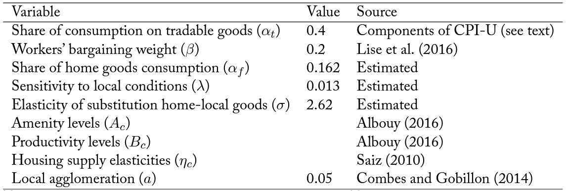
Notes: This table shows the estimates of the structural parameters of the model. The structural parameters of the model are the set of parameters that minimize the distance between the model and the data. For this exercise we only use data on wages and distributions of workers across locations at the country-of-origin level, taking as given the parameters borrowed from prior literature.
5.7 Comparison model vs. data
Once we have all the parameters – those that we estimate ourselves and those that we borrow from the literature – we can compare the quantitative predictions of our model with the data. Using various moments of the data should serve to show that our model can quantitatively match some of the key features of metropolitan-level cross-sectional US data. We demonstrate this below.
At an aggregate level, the model estimated exclusively on labor market data delivers an estimate of the weight of the home country on overall consumption that is not far from the direct estimates that we obtained using Consumer Expenditure Survey data. In section 3.4.3, we have shown that Mexican households consume on average 12 percent less on local goods than similar-looking natives. We can directly compare this estimate with the estimate  .51One reason for the somewhat lower estimate from the Consumer Expenditure Survey could be that there are also some natives among the Mexican households that we use to proxy for immigrant households. This attenuates the effect on expenditure, if the consumption of native Mexican households is similar to that of non-Mexican households.
At a disaggregated MSA level, we can compare the predictions of the model with the data. In figure 9, we plot a number of variables against city productivity levels. Note that our estimation of the model is at the city-country of origin level, while the moments in figure 9 are at the MSA level. The underlying productivities, amenities, and price levels are the primitive parameters that drive the results on both location and wages. Appendix table E.1 gives an overview over these parameters for the bottom 20 and the top 20 cities in terms of productivity.
The top-left graph in figure 9, labeled as panel A, shows that the population distribution across US cities generated by the model is very similar to the distribution in the data both in terms of steepness and dispersion. The model only performs somewhat worse at the extremes of the distribution. It underpredicts the size of the two largest cities, which are New York and Los Angeles, while it somewhat overpredicts the size of the smallest cities.
The model matches remarkably well the relationship between wages (centered around the mean) and productivity as shown in panel B of figure 9. In appendix C.2 we show that this fit does not change substantially with alternative calibrations of β and .
Figure 9. Model and data, MSA-level moments
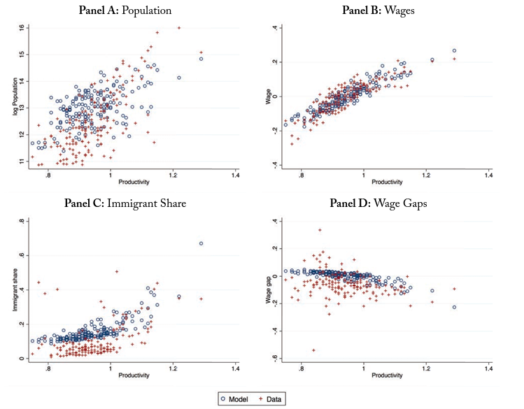
Notes: This figure compares four untargeted moments in the data and the model. The model is estimated using country of origin variation. From these estimates, we aggregate to the city level the data generated by the model to compute the four moments shown in the figure. Each dot represents a city. We use the 168 consolidated metropolitan statistical areas from Albouy (2016).
The model also does a fairly good job in explaining the immigrant population shares and native-immigrant wage gaps (aggregated at the city level). That is, the model predicts productivity to be positively related to immigrant shares and negatively related to immigrants’ relative earnings, mimicking the relationships in the data. Naturally, there is less dispersion in the model than in the data, as all differences between locations of similar productivity are only based on variation in amenities and non-tradable prices, while in the real world there are many more sources of heterogeneity that drive immigrant shares and wage gaps.
It is interesting to see that there are some outliers in terms of immigrant shares. The smaller MSAs with high shares of immigrants in the data are always close to the Mexican border. This is something that the model cannot match. Another outlier with respect to the prediction is the most productive city, San Francisco, for which the model predicts an immigrant share of around 67 percent – almost twice as high as in the data. San Francisco is a special case because it is at the extreme end of the distribution with respect to all of its characteristics (see table E.1). It is the most productive city and has the highest rental price index by a large margin. Moreover, it has the second highest amenity value (after Santa Barbara) and the second lowest housing supply elasticity (after San Diego). Naturally, for such a location, the model predicts an extreme outcome in terms of the number of immigrants, who are attracted by the high nominal wage driven by both the exceptionally high productivity and high non-tradable price level. Because of the large discrepancy between data and model for this special case, we drop San Francisco from the counterfactual analysis that we perform in the next section.
Overall, apart from these few outliers, it seems that our estimated model is quantitatively similar to the data, and can thus be used to perform some counterfactual experiments that should help to shed light on the importance of immigrants in a number of outcomes.
5.8 The distribution of economic activity and general equilibrium
The counterfactual exercise that we undertake is to examine changes in the equilibrium that arise after an increase in the share of immigrants, holding total population and the distribution of countries of origin constant. We perform this counterfactual because it cleanly shows the quantitative importance of the mechanism that we highlight throughout the paper. More specifically, we first compute the distribution of population across MSAs and equilibrium prices and wages assuming that immigrants consume and therefore decide on locations exactly like natives. Second, we do the same exercise with current immigration levels of around 20 percent. From these two exercises we calculate percentage differences in outcome variables of interests to quantify the contribution of immigrants’ choices to the equilibrium. We perform this exercise both with and without agglomeration forces (i.e., with a = 0 and a = 0.05 in equation 5.3). We show the main results in figure 10.
Figure 10. Effects of immigrants’ location choices
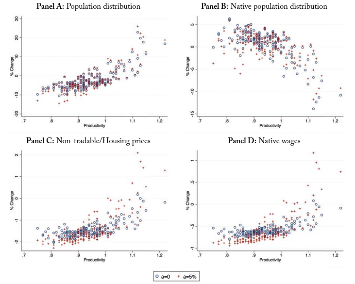
Notes: This figure compares the distribution of selected variables predicted by the model with the actual share of immigrants of 20 percent and the counterfactual distribution predicted if all immigrants consume like natives, both with and without agglomeration forces. Each dot represents one of the 168 consolidated metropolitan statistical areas from Albouy (2016) and indicates the percentage difference to the counterfactual.
It is apparent from panel A that migration increases the size of the most productive cities at the expense of the least productive cities. These gains and losses are accentuated in the presence of positive agglomeration forces. The most productive MSAs in the United States are around 10 percent-25 percent larger than they would be if immigrants decided on locations in the way natives do.52The predicted population change for the dropped outlier San Francisco is around 75 percent. Even if the population in the metropolitan statistical area of San Francisco has almost doubled over the last 50 to 60 years, this is a rather unrealistic prediction.
As a result of immigrants’ strong preference for cities with high nominal wages and the pressure that this puts on local price indices, which can be seen in panel C, natives are displaced from more productive cities into less productive ones as shown in panel B.53Note that we correct this plot for the fact that native population falls when we convert natives to immigrants, and therefore every city mechanically has 20 percent fewer natives. In fact, current levels of migration can potentially account for a significant part of the increase in local price indices in more productive cities. Note that price changes are more pronounced at the extremes if there are agglomeration forces, which is due to the stronger effects on population resulting from the additional productivity changes. Without agglomeration forces, prices rise only in one city (Santa Barbara), while they fall in all the remaining ones, even in those that see their population rise. This is because immigrants demand fewer non-tradable goods than natives, and this negative effect on demand resulting from the different composition of population overcompensates for the positive effect resulting from more population. Despite the fall in prices in (most of ) the high-productivity cities, some natives leave those cities because prices fall more in low-productivity cities, making the low-productivity cities relatively more attractive.
However, as panel B shows, there are also a few low-productivity cities that lose in terms of native population. This is a consequence of the fact that at the lower end of the productivity distribution, there are some cities with very high housing supply elasticities, which implies weaker price declines with falling demand. These cities become less attractive relative to cities with larger prices drops due to lower housing supply elasticities, even if productivity is comparable.
Panel D of figure 10 shows that natives’ wages move in the same direction as local price levels. Without agglomeration forces, immigrants’ location choices do not lead to substantial wage changes in more productive locations, and they lead to slight declines in less productive ones. With agglomeration forces, the wage changes are more strongly increasing in productivity. It is remarkable to note that immigrants’ location choices also help to explain the divergence in nominal incomes between metropolitan statistical areas, in line with the evidence reported in Moretti (2013). With agglomeration forces, both housing prices and nominal wages increase with immigration. In the context of the model, however, real-wage inequality between small and large locations does not increase since price changes are more pronounced than nominal wage changes.
In figure 11, we investigate the effect of immigrants, going up to a share of 40 percent, on some aggregate variables. We have shown that immigration moves economic activity from low-productivity locations to high-productivity ones. As a result, an immigrant share of 20 percent increases average labor productivity (i.e., tradable output produced per worker) by around 0.9 to 1 percent, depending on whether agglomeration forces are considered or not. Thus, the growth in size of the most productive cities translates into output gains for the tradable sector in the entire economy, even if low-productivity places lose.
In panel B of figure 11, we investigate native workers’ welfare, measured as the common component of the indirect utility of natives expressed in equation 5.1,  . On aggregate, native workers’ welfare increases by around 0.35 percent.54Recall that we abstract from the welfare changes of firm and land owners, which are not modeled. This change is driven by various forces. First, wages fall on average due to lower non-tradable prices. This is a consequence of the fact that immigrants spend less than natives on local non-tradables. Since the relative price of non-tradables falls, natives consume more non-tradabales, which tends to raise their welfare. However, since wages are lower, they also consume fewer tradable goods, which tends to reduce their welfare. Because the drop in the nominal wage is less pronounced than the drop in price levels, real wages and thus native welfare always increase. The welfare effects are slightly lower with agglomeration effects since some natives move to the low-productivity cities (with a few exceptions), which lose in terms of overall population. Therefore, these cities have a lower productivity compared to the case without agglomeration forces, which drives natives’ nominal wages in these cities further down.
Figure 11. Aggregate effects of immigrants
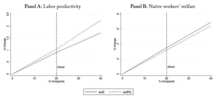
Notes: This figure compares aggregate macroeconomic variables predicted by the model under the current level of immigration with those predicted assuming that immigrants behave identically to natives. Panel A shows the aggregate change in worker productivity resulting from the re-shaping of economic activity across space at different levels of immigration. Panel B shows the change in aggregate native workers’ welfare.
In appendix C.2, we perform robustness checks to show that these disaggregate and aggregate predictions from the model do not change substantially with alternative calibrations of β and .
6 Conclusion
In the first part of this paper, we document that immigrants concentrate in larger, more expensive cities and that their earnings relative to natives are lower there. We show that these patterns are stronger for immigrants coming from low-price index countries and that immigrants relative to similar-looking native households consume less locally.
Taking all this evidence together, we posit that these patterns emerge because a share of immigrants’ consumption is not affected by local price indices but rather by prices in their country of origin. That is, given that immigrants send remittances home and are more likely to spend time in and consume in their countries of origin, they have a greater incentive than natives to live in high-nominal-income locations.
We build a quantitative spatial equilibrium model labor market with frictions to quantify the importance of this mechanism. We estimate the model and show that the differential location choices of immigrants relative to natives have important consequences: economic activity moves from low-productivity places to high-productivity places, which leads to a gain in overall worker productivity of around 1 percent and increases native welfare by around 0.35 percent, at current levels of immigration.
This paper extends some of the insights in the seminal contribution of Borjas (2001). Borjas’ main argument is that immigrants choose the locations where demand for labor is higher, thus helping to dissipate arbitrage opportunities across local labor markets. We show in this paper that immigrants not only choose locations with higher demand for labor but specifically more productive locations, and we quantify how much these choices contribute to overall production in the United States.
References
Ahlfeldt, G., S. Redding, D. Sturm, and N. Wolf, “The Economics of Density: Evidence from the Berlin Wall,” Econometrica, 2015.
Albert, Christoph, “The Labor Market Impact of Undocumented Immigrants: Job Creation vs. Job Competition,” CESifo Working Paper Series 6575, CESifo Group Munich October 2017.
Albouy, D., “The Unequal Geographic Burden of Federal Taxation,” Journal of Political Economy, 2009.
, “What are Cities Worth? Land Rents, Local Productivity, and the Total Value of Amenities,” Review of Economics and Statistics, 2016, 98(3), 477–487.
, H. Cho, and M. Shappo, “Immigration and the Pursuit of Amenities,” mimeo, 2018.
Altonji, J. and D. Card, The Effects of Immigration on the Labor Market Outcomes of Less-Skilled Natives, in John Abowd and Richard Freeman (eds.), Immigration, Trade, and the Labor Market, University of Chicago Press, 1991.
Angelucci, M., “Migration and financial constraints: evidence from Mexico,” The Review of Economics and Statistics, 2015, 97 (1).
Autor, D., D. Dorn, and D. Hanson, “The China Syndrome: Local Labor Market Effects of Import Competition in the United States,” American Economic Review, 2013, 103(6), 2121–2168.
Bartel, Ann, “Where Do the New U.S. Immigrants Live,” Journal of Labor Economics, 1989, 7, 371–391.
Baum-Snow, N. and R. Pavan, “Understanding the City Size Wage Gap,” Review of Economic Studies, 2012, 79(1), 88–127.
Becker, G., The Economics of Discrimination 1957.
Black, D., “Discrimination in an equilibrium search model,” Journal of Labor Economics, 1995.
Borjas, G., “Assimilation, Changes in Cohort Quality, and the Earnings of Immigrants,” Journal of Labor Economics, 1985.
, “Does Immigration Grease the Wheels of the Labor Market?,” Brookings Papers on Economic Activity, 2001.
, “The Labor Demand Curve is Downward Sloping: Reexamining the Impact of Immigration on the Labor Market,” Quarterly Journal of Economics, 2003, pp. 1335–1374.
, “The Slowdown in the Economic Assimilation of Immigrants: Aging and Cohort Effects Revisited Again,” Journal of Human Capital, 2015.
, We wanted workers 2016.
, “The Earnings of Undocumented Immigrants,” NBER Working Papers 23236, National Bureau of Economic Research, Inc Mar 2017.
, “The Labor Supply of Undocumented Immigrants,” Labour Economics, Forthcoming.
and J. Monras, “The Labor Market Consequences of Refugee Supply Shocks,” Economic Policy, 2017, 32(91), 361–413.
, R. Freeman, and L. Katz, “How Much Do Immigration and Trade Affect Labor Market Outcomes?,” Brookings Papers on Economic Activity, 1997, pp. 1–67.
Burstein, A., G. Hanson, L. Tian, and J. Vogel, “Tradability and the Labor-Market Impact of Immigration: Theory and Evidence from the U.S.,” mimeo, 2018.
Cadena, B. and B. Kovak, “Immigrants Equilibrate Local Labor Markets: Evidence from the Great Recession,” American Economic Journal: Applied Economics, 2016.
Caliendo, L., F. Parro, E. Rossi-Hansberg, and P-D. Sartre, “The Impact of Regional and Sectoral Productivity Changes on the U.S. Economy,” Review of Economic Studies, Forthcoming.
, M. Dvorkin, and F. Parro, “Trade and Labor Market Dynamics,” NBER Working Paper No. 21149, 2015.
Card, D., “The Impact of the Mariel Boatlift on the Miami Labor Market,” Industrial and Labor Relations Review, 1990, pp. 245–257.
, “Immigrant Inflows, Native Outflows and the Local Labor Market Impacts of Higher Immigration,” Journal of Labor Economics, 2001, 19.
, “Is The New Immigration Really So Bad?,” Economic Journal, 2005, 115, 300–323.
, “Immigration and Inequality,” American Economic Review Papers and Proceedings, 2009, 99(2), 1–21.
Chiswick, B., “The Effect of Americanization on the Earnings of Foreign-born Men,” Journal of Political Economy, 1978, 86(5), 897–921.
Combes, P-P. and L. Gobillon, “The Empirics of Agglomeration Economies,” Handbook of Regional and Urban Economics, 2014.
Cortes, P., “The Effect of Low-skilled Immigration on U.S. Prices: Evidence from CPI Data,” Journal of Political Economy, 2008, pp. 381–422.
Davis, D. and J. Dingel, “The Comparative Advantage of Cities,” NBER Working Paper 20602, 2012.
Davis, S. and T. von Wachter, “Recessions and the Costs of Job Loss,” Brookings Papers of Economic Activity, 2011.
de la Roca, J. and D. Puga, “Learning by working in big cities,” Review of Economic Studies, 2017, 84(1), 106–142.
Diamond, R., “The Determinants and Welfare Implications of US Workers’ Diverging Location Choices by Skill: 1980-2000,” American Economic Review, 2015.
Duranton, G., “Urban evolutions: The fast, the slow, and the still,” American Economic Review, 2007, 97(1), 197–221.
and D. Puga, “Micro-Foundations of Urban Agglomeration Economies,” Handbook of Regional and Urban Economics, ed. Hendersson and Thisse, 2004.
Dustmann, C., “Return migration, uncertainty and precautionary savings,” Journal of Development Economics, 1997.
, “Return migration, wage differentials, and the optimal migration duration,” European Economic Review, 2003.
and J. Mestres, “Remittances and Temporary Migration,” Journal of Development Economics, 2010, 92(1), 70–62.
and JS. Gorlach, “The economics of temporary migrations,” Journal of Economic Literature, 2016.
and Y. Weiss, “Return Migration: Theory and Empirical Evidence from the UK,” British Journal of Industrial Relations, 2007.
, U. Schonberg, and J. Stuhler, “The Impact of Immigration: Why Do Studies Reach Such Different Results?,” Journal of Economic Perspectives, 2016.
, , and , “Labor Supply Shocks and the Dynamics of Local Wages and Employment,” Quarterly Journal of Economics, 2017.
Eeckhout, J. and N. Guner, “Optimal Spatial Taxation: Are Big Cities too Small?,” mimeo, 2014.
, R. Pinheiro, and K. Schmidheiny, “Spatial Sorting,” Journal of Political Economy, 2014, 122(3), 554–620.
Fajgelbaum, P., J.C. Morales E. Suarez-Serrato, and O. Zidar, “State Taxes and Spatial Misallocation,” mimeo, 2016.
Giovanni, J. Di, A. Levchenko, and F. Ortega, “A Global View of Cross-border Migration,” Journal of the European Economic Association, 2015.
Glaeser, E., Cities, Agglomeration and Spatial Equilibrium, Oxford University Press, 2008.
Glitz, A., “The Labor Market Impact of Immigration: A Quasi-Experiment Exploiting Immigrant Location Rules in Germany,” Journal of Labor Economics, 2012, 30(1), 175–213.
Handbury, J., “Income and Quality: Lessons from Micro Data for Estimating Aggregate Welfare,” mimeo Columbia, 2011.
and D. Weinstein, “Goods Prices and Availability in Cities,” Review of Economic Studies, 2015, 82 (1), 258–296.
Hanson, G., “Illegal Migration from Mexico to the United States,” Journal of Economic Literature, 2006, 44(4), 869–924.
Hsieh, C-T. and E. Moretti, “Housing Constraints and Spatial Misallocation,” mimeo, 2017.
Jaeger, D., “Green Cards and the Location Choices of Immigrants in the United States, 1971-2000,” Research in Labor Economics, 2007.
, J. Ruist, and J. Stuhler, “Shift-share Instruments and the Impact of Immigration,” NBER working paper, 2018.
Jarosch, G., “Searching For Job Security and the Conseuquences of Job Loss,” RR Econometrica, 2016.
Lach, S., “Immigration and Prices,” Journal of Political Economy, 2007.
Lessem, R., “Mexico-U.S. Immigration: Effects of Wages and Border Enforcement,” Review of Economic Studies, Forthcoming.
Lewis, E., “Immigration, Skill Mix, and Capital-Skill Complementarity,” Quarterly Journal of Economics, 2012, 126(1), 1029–1069.
Lise, J., C. Meghir, and J.M. Robin, “Matching, Sorting and Wages,” Review of Economic Dynamics, 2016, 19(1).
Llull, J., “The Effect of Immigration on Wages: Exploiting Exogenous Variation at the National Level,” Journal of Human Resources, 2017, Forthcoming.
Manacorda, M., A. Manning, and J. Wadsworth, “The Impact of Immigration on the Structure of Male Wages: Theory and Evidence from Britain,” Journal of the European Economic Association, 2012, 10(1), 120–151.
Manning, A., “Imperfect Competition in the Labor Market,” Handbook of Labor Economics, 2011.
Monras, J., “Economic Shocks and Internal Migration,” IZA Discussion Paper No. 8840, 2015.
, “Immigration and Wage Dynamics: Evidence from the Mexican Peso Crisis,” IZA Discussion Paper No. 8924, 2015.
Monte, F., F. Redding, and E. Rossi-Hansberg, “Commuting, Migration and Local Employment Elasticities,” mimeo, 2015.
Moretti, E., “Real Wage Inequality,” American Economic Journal: Applied Economics, 2013.
Munshi, K., “Networks in the Modern Economy: Mexican Migrants in the U.S. Labor Market,” Quarterly Journal of Economics, 2003.
Nekoei, A., “Immigrants’ Labor Supply and Exchange Rate Volatility,” American Economic Journal: Applied Economics, 2013, 5 (4), 144–164.
Notowidigdo, M., “The Incidence of Local Labor Demand Shocks,” mimeo, 2013.
Oreopoulos, P., T. von Wachter, and A. Heisz, “Short- and Long-Term Career Effects of Graduating in a Recession,” American Economic Journal: Applied Economics, 2012.
Ottaviano, G. and G. Peri, “Rethinking the Effect of Immigration on Wages,” Journal of the European Economic Association, 2012, 10 (1), 152–197.
Patel, Krishna and Francis Vella, “Immigrant Networks and Their Implications for Occupational Choice and Wages,” The Review of Economics and Statistics, October 2013, 95 (4), 1249–1277.
Piyapromdee, S., “The Impact of Immigration on Wages, Internal Migration and Welfare,” mimeo UCL, 2017.
Redding, S., “Goods trade, factor mobility and welfare,” Journal of International Economics, 2014.
and E. Rossi-Hansberg, “Quantitative Spatial Economics,” Annual Review of Economics, Forthcoming.
Redding, Stephen and Daniel Sturm, “The Costs of Remoteness: Evidence from German Division and Reunification,” American Economic Review, 2008, 98(5), 1766–1797.
Ruggles, S., M. Sobek, T. Alexander, C.A. Fitch, R. Goeken, PK Hall, M. King, and C. Ronnander, “Integrated Public Use Microdata Series: Version 4.0 [Machine-readable database].,” Minneapolis, MN: Minnesota Population Center [producer and distributor], 2016.
Saiz, A., “Room in the Kitchen for the Melting Pot: Immigration and Rental Prices,” Review of Economics and Statistics, 2003, 85(3), 502–521.
, “Immigration and housing rents in American cities,” Journal of Urban Economics, 2007, 61(2), 345–371.
, “The Geographic Determinants of Housing Supply,” Quartely Journal of Economics, 2010, 125(3), 1253–1296.
and S. Wachter, “Immigration and the Neighborhood,” American Economic Journal: Economic Policy, 2011, 3(2), 169–188.
Silva, J.M.R. Santos and S. Tenreyro, “The log of Gravity,” Review of Economics and Statistics, 2006, 88(4), 641–658.